
Abstract
This article investigates a novel method for time-varying systems with an impact term; we call it a modified homogenized highly precise direct integration method. Modified homogenized highly precise direct integration method can deal with the time-varying nonhomogeneous systems effectively by direct integration with high precision. Even though it is often difficult to select the time step size of integration properly for stiff problems, modified homogenized highly precise direct integration method can effectively deal with the this problem with a large time step size. By introducing new variants twice, modified homogenized highly precise direct integration method can easily deal with the nonhomogeneous term by a novel way, inherit the advantages of highly precise direct integration method and avoid the calculation of inverse matrix. The convergency and efficiency analyses are given in this article. Several numerical simulations and an application example are presented to demonstrate the high accuracy, effectiveness and application for engineering problems of modified homogenized highly precise direct integration method.
Keywords
Introduction
Time-varying dynamic problems arise in many areas of structural analysis, such as vehicle bridge interactive systems, rockets or aircraft systems. The dynamic response of the structure can be analysed by the direct integration methods (the Newmark-α method, 1 Wilson-θ method 2 or Houbolt schemes) or transferring the system into first-order evaluation problems (the Runge–Kutta, spectral deferred correction,3,4 time discontinuous Galerkin methods 5 ). However, for some stiff problems, 6 the time step size should be selected carefully, which makes these methods time-consuming.
Highly precise direct integration (HPD) 7 method was proposed for homogeneous linear time-invariant dynamic systems. Due to its advantages of high precision and high efficiency, HPD had been widely applied to many problems. When applied to the linear ordinary differential equations (ODEs), HPD provided the numerical solution up to the machine precision, and it was an efficient and stable method. In order to solve the nonhomogeneous systems with high precision, expanding dimension methods8,9 were proposed. These methods deal with the nonhomogeneous terms by different function expansions, such as Fourier, Legendre or Chebyshev expansions. However, for expanding dimension methods, there were several drawbacks including too many variants introduced, large dimension and low accuracy. In this article, we propose modified homogenized method, which can avoid these drawbacks.
However, perturbation method was presented in the study of Tan and Zhong 10 recently, where the original time-varying system was decomposed into two sub-Hamiltonian systems, that is, a zero-order system and a perturbation one. A high-order multiplication perturbation method (HOMPM) 11 was presented, in which a low-order perturbation system was decomposed into a low-order system and a high-perturbation system by variable transformation. Each subsystem can be solved by HPD, and the solution can be determined through a series of inverse transformations. However, it is time-consuming to compute the high precise matrix in every small interval. To solve variable coefficient singularly perturbed two-point boundary value problems, HOMPM 12 was put forward. But HOMPM encounter the similar problems as HPD. Another idea to improve the accuracy is time-adaptive methods. For mass-variant systems (the flight of rockets), adaptive methods were presented in the study of Wang and colleagues,13,14 which selected the time step size or the order of the proposed method adaptively. Methods15,16 for periodic time-varying systems were put forward, in which the precise transferred matrix in the first period was expressed by the theory of Peano–Baker series and used in the following periods. This method was only suitable for the periodic problems. For general problems, it may cost too much computation and computer’s memory.
In this article, we propose a modified homogenized highly precise direct (MHHPD) integration method. This method is efficient for a class of time-varying nonhomogeneous systems, whose coefficients matrices are polynomials, and nonhomogeneous term is complicated. Briefly, we can summarize the method into three steps as follows:
Transfer the nonhomogeneous systems into homogeneous ones by expanding dimensions via novel methods;
Convert the transferred time-varying homogeneous systems into time-invariant systems by introducing several variants;
Utilize the standard HPD method for the transferred homogeneous time-invariant systems.
The transfer matrix is generated once and used forever, which is efficient and accurate. The accuracy of the proposed method is studied and proved by comparing with those of the others which are used commonly (e.g. RK4, Radau5, 17 Newmark-α, 1 ode15s, 18 Wilson-θ2).
Time-varying systems and their homogenized forms
In this section, we will provide the basic equation of structural dynamic problems with four different types of nonhomogeneous terms and their related homogenized forms. In the past decades, expanding dimension methods8,19–22 were widely used for the nonhomogeneous dynamic systems. The nonhomogeneous loading form could be classified into three types: the polynomial loading form, the sinusoidal loading form, and the arbitrary loading form. However, the accuracy of these expanding dimension methods relates to the serials expansion caused by the truncation errors. For complicated loading terms, many dimensions need to be introduced, which is time and memory consuming. Therefore, a new type expanding dimension method is proposed in this section. For some typical loading forms, MHHPD are much more accurate.
The time-varying structural dynamic systems
The equation of motion for N-degree-of-freedom (N-DOF) time-varying dynamic systems can be expressed in a matrix form as
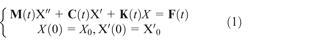
where
Let

where
The novel homogenized method
For the nonhomogeneous system (equation (2)), function expansions are the typical ways for the nonhomogeneous term. For the complicated loading forms
Case 1.
If

where
Case 2.
If pn(t) is a polynomial scalar function of degree not exceeding n and

where
Case 3.
If

where
Case 4.
If pn(t) is a polynomial scalar function of degree not exceeding n,

where
From equations (3)–(6), we can summarize that the nonhomogeneous systems can be homogenized into the same form, as follows

where

MHHPD
In this section, we introduce MHHPD more in detail and analyse the convergence of this method. The nonhomogeneous system (equation (2)) with coefficient
Definition 1
For 0 < ρ < 1 and
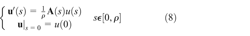
Then, equation (8) is called unit time-varying system,

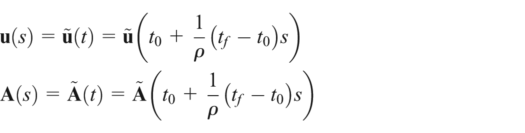
Then, the time interval [t0, tf] can be mapped into [0, ρ], with the initial value s(t0) = 0. According to equation (9), we can get the related
We can make the conclusion that system equations (7) and (8) are equivalent.
Expanding dimensions for the time-varying systems
This subsection introduces how to deal with the time-varying coefficient
Let

and

where, r is the degree of
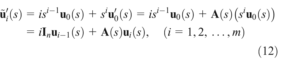

Hence, a combination of equations (8)–(13) leads to

where
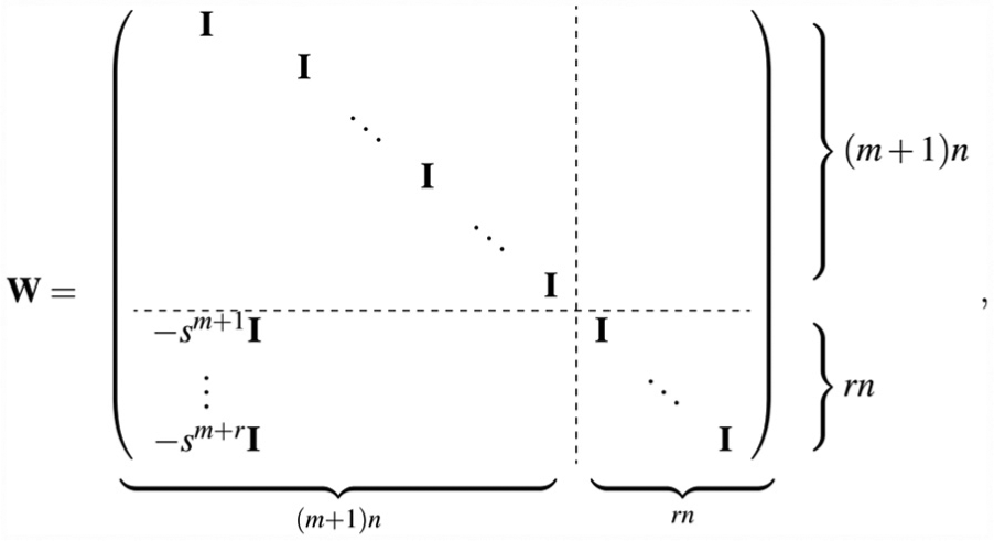

Then, the time-varying coefficient matrix
Convergence
In this subsection, we will study the convergence of MHHPD. To this end, we give the following.
Definition 2
If

is called time-invariant homogeneous system, where
In the views of some studies,9,21 equations (2) and (7) are equivalent for the expanding dimension method.
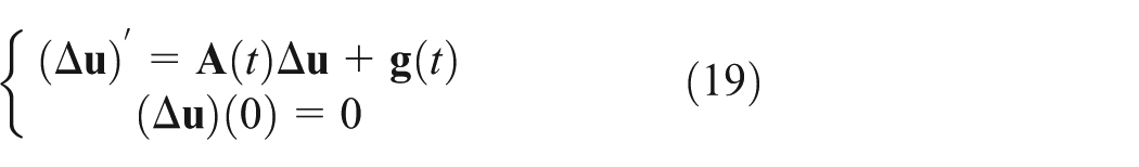
Theorem 1
When ε(t) → 0, the solution of

converges to the solution

Proof
By equations (16) and (17), we obtain

where
Let
Hence

So, as ε(t) → 0, the solution of equation (16) converges to the solution of equation (17).
Theorem 2
When m → +∞, the solution of equation (14) converges to the solution of equation (15).
Proof
A combination of equations (14) and (15) leads to

Furthermore, we partition matrices
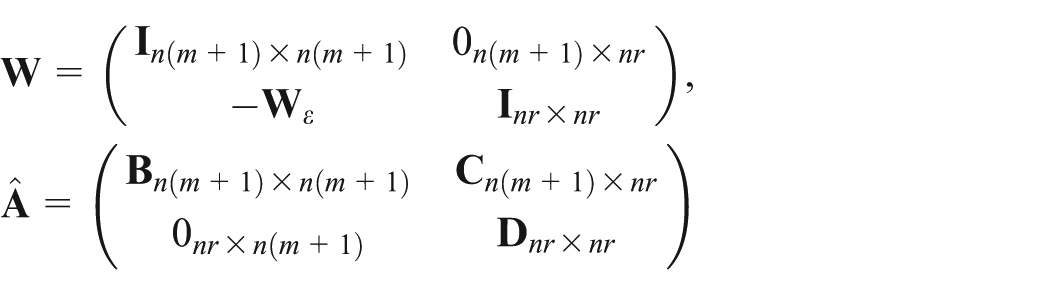
where

It follows that
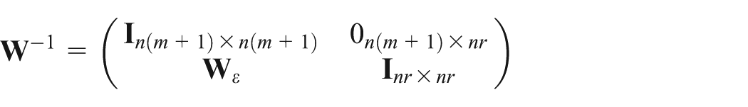
Moreover

Therefore

This, together with equation (8), leads to

Hence, we obtain

with the initial conditions
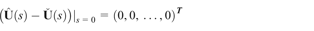
Finally, all the above yields

HPD method for the transferred systems
Equation (15) is a homogenized time-invariant system, standard HPD can be used. The solution of equation (15) can be written as

If τ is taken as step size of the time, that is,

where

As
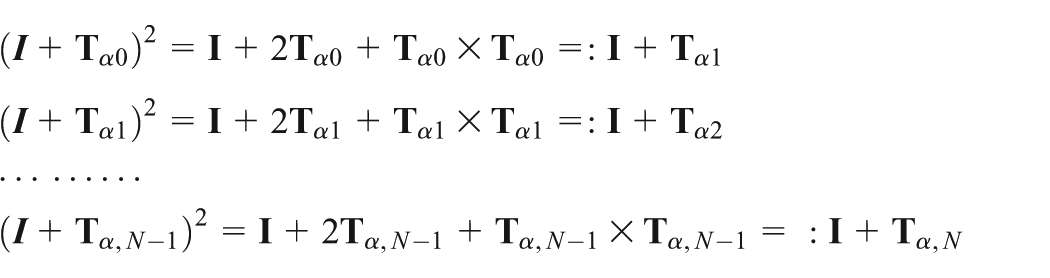
In order to compute

where
Furthermore, the precision parameter N should be selected previously (e.g. N = 20). Then

Furthermore
It is clear that

The procedure for computing
HPD.

Finally, we give the procedure of MHHPD in Algorithm 2 MHHPD.
MHHPD.

Efficiency analysis
For the dynamical problems, especially, the stiff problems, we have to select a small time step size for stability. There is no doubt, small time step size costs lots of computation. MHHPD method inherits the advantages of HPD method and can calculate the stiff problem by large time step. Even though MHHPD is a bit complicated before using the standard HPD method, it is worthy for us compared to the time cost with different methods. Therefore, in this subsection, we roughly estimate the cost time of MHHPD and compare the cost with traditional one-step method (e.g. Newmark-β method). To begin with, we assume that the cost of each step is identical for both MHHPD and traditional one.
First, we assume that the high precise parameter is N, and the time step size is dt. We take the

However, for traditional methods, 2 N sub-steps have to be calculated for equivalent accuracy within every time interval

Based on the analysis hereinbefore, the time cost of the traditional method is about
Solving process
Let t = tk+1. The numerical solution of equation (15) is
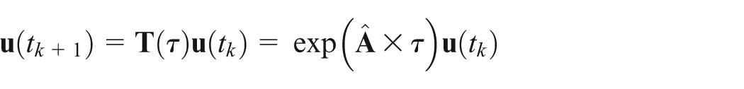
Using Algorithm 1 HPD, the solution
Finally, the unit interval needs to be transformed into the original interval by an inverse transform

Numerical simulations
In this section, we present several numerical results to illustrate the advantages of MHHPD.
A first-order time-varying nonhomogeneous system
We show the steps and efficiency of MHHPD by a simple example for a better understanding
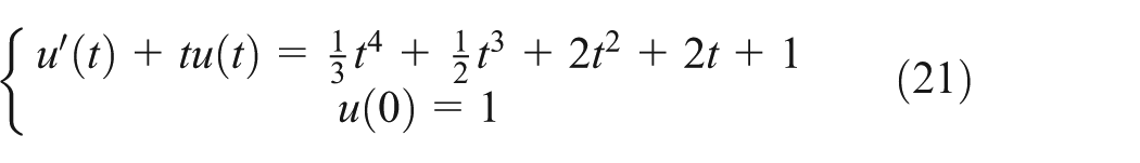
The exact solution is given by

We solve equation (21) using MHHPD method and fourth-order Runge–Kutta (RK4 23 ) method with different time step sizes.
We present several necessary steps of MHHPD in detail as follows:
Homogenize the systems. By expanding dimension method, equation (21) can be homogenized as follows

where

Transfer the time-varying system into time-invariant one. As the highest degree of the polynomial coefficient

where

Utilize HPD method. Algorithm 1 can be used for the high precision.
In Table 1, the comparison of the numerical errors between RK4 and MHHPD under the same time step size is given. It can be observed that MHHPD is much more accurate than RK4. It is also shown in Table 1 that time step size h has little influence on the numerical error of MHHPD. If h is fixed, as the expand dimension parameter m increases, the error decreases. However, when m > 10, m has little influence on the accuracy.
Simulation 5.1 – comparison of errors with MHHPD (N = 20) and RK4.

MHHPD: modified homogenized highly precise direct integration method.
In Table 2, the influence of dimensional expanding parameter m and precision parameter N is discussed. For time-invariant systems, the selection of precision parameter N was discussed in Tan et al. 24 For the time-varying system (equation (21)), N has little influence on the accuracy. If m < 10, as m increases the error decreases; but when m > 10, the errors no longer decrease, as m increases, so there is no need for a bigger m.
Simulation 5.1 – comparison of errors with MHHPD (h = 0.1) with different dimensional expanding m and different parameter N.
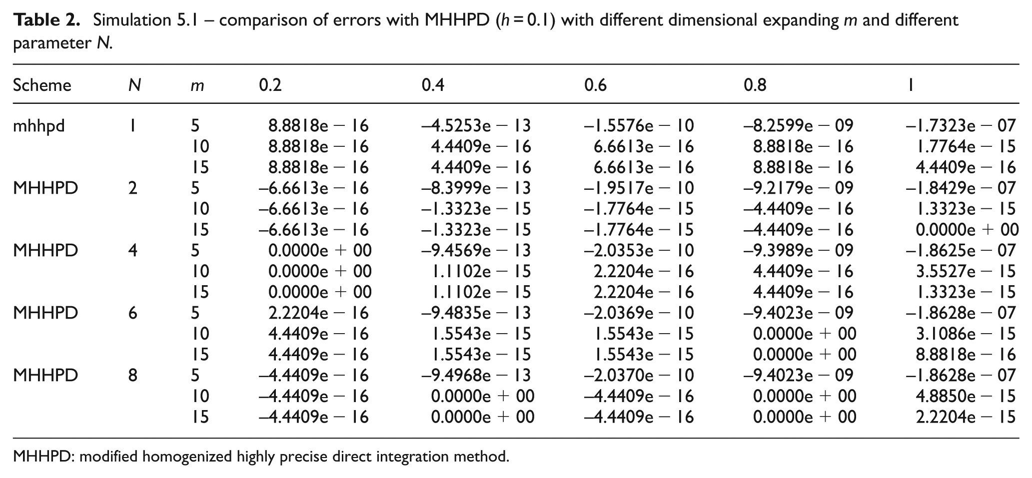
MHHPD: modified homogenized highly precise direct integration method.
A time-varying nonhomogeneous system with multi-frequency
For the multi-frequency systems, the canonical equations are stiff. So, the time step size has to be selected carefully. 6 Since MHHPD is insensitive to the time step size, it is convenient for this problem.
Consider the system

where
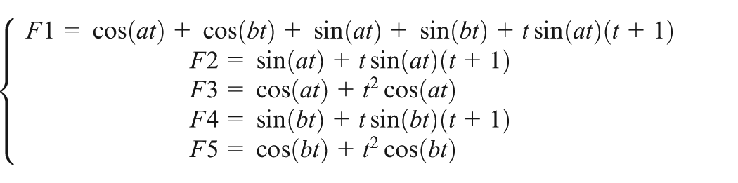
The exact solution is given by

Equation (22) is a multi-frequency system, and the parameters a and b represent the different frequencies. We take a = 10 and b = 10,000 as an example. Few numerical methods can solve this system with big time step size. For a better comparison, we apply MHHPD (N = 35; m = 40) with time step size h = 0.01, time-adaptive methods (Radau5 17 and ode15s 18 ) and RK4 with time step size h = 10−6 for this problem.
For the multi-frequency problem, traditional methods can simulate the low frequency very well; however, for the high frequency, things changed, the time step size has to be small enough for a better solution. In our simulation, the solutions of MHHPD and traditional methods are equivalent in the aspect of low-frequency part. In Figures 1–3, the numerical solutions by mentioned methods are presented for the high-frequency part. The right one is the exact solutions, and the left ones are the numerical solution. Radau5 is an adaptive method, and we choose the relative error and absolute error as 10−6, and the number of computational points is 6132. Similarly, ode15s is an adaptive method; the relative error and the absolute error are the same as Radau5, and the number of computational points is 119,707. RK4 is an explicit method, which needs tiny time step size h = 10−6 for a good solution. The time step size of MHHPD is relatively big h = 0.01. As shown in Figures 1–3, although the time step size of MHHPD is big, MHHPD is more accurate than traditional methods.

Simulation 5.2 – the numerical solution of u1 obtained by compared methods: (a) the exact solution and (b) numerical solutions.

Simulation 5.2 – the numerical solution of u4 obtained by compared methods: (a) the exact solution and (b) numerical solutions.

Simulation 5.2 – the numerical solution of u5 obtained by compared methods: (a) the exact solution and (b) numerical solutions.
In Table 3, the errors and CPU time are presented. MHHPD is an explicit method and has fewer computational costs and is much more efficient than the traditional methods.
Simulation 5.2 – comparison of the errors by different methods.

MHHPD: modified homogenized highly precise direct integration method.
A nonhomogeneous Hermite equation
Consider the nonhomogeneous Hermite equation
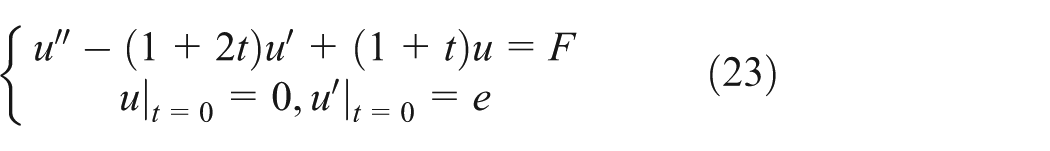
We consider a complicate form of F
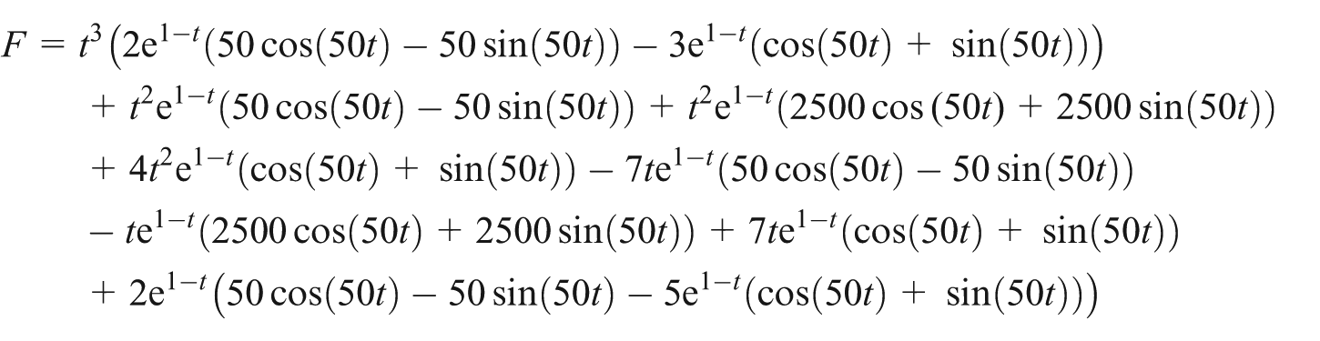
Equation (23) has the exact solution

Taylor or Chebyshev series expansions of F(t) are recommended in the literature.20–22 Because of truncation errors, when using the recommended methods, we have to introduce many dimensions, which unavoidably cost memories. MHHPD can avoid the large dimension and the truncation error.
This simulation has been carried out with different time integration schemes: MHHPD (N = 15;m = 30), fourth-order Runge–Kutta, Newmark method (with α = 0.25; β = 0.5), 1 Wilson method (with θ = 1.4), 2 Radau5 and ode15s. RK4 method, Newmark method (with α = 0.25; β = 0.5) and Wilson method (with θ = 1.4) apply the same time step size h = 10−6. Radau5 and ode15s are time-adaptive methods; we choose the relative error and absolute error as 10−8.
MHHPD is an explicit method; the transfer matrix T is calculated once and used forever, so it is efficient on this problems. In Table 4, the numerical errors and CPU time (in s) of different schemes are compared. It can be observed that the cost of CPU time of MHHPD method is much less than other methods. In addition to this, MHHPD method provides much more accurate numerical results.
Simulation 5.3 – the errors and CPU time by different methods.

MHHPD: modified homogenized highly precise direct integration method.
The precision parameter N and dimensional expanding parameter m play important roles for the computation. The selection of N for the HPD method was discussed. 24 The influence of m and N is presented in Figure 4. As N increases, the sub-step τ = h/2 N and the errors decrease. However, as shown in Figure 4, when N > 15, the increase in N has little influence to the accuracy. Meanwhile, the parameter m, namely, the expanding dimensions, relates to the accuracy and has the following regularities: when m < 10, the bigger the m, the higher the accuracy, and while m ∈ (10, 20), the errors are the lowest; however, when m > 20, as m increases, the accuracy decreases, which is mainly caused by the computer’s round-off error. 25 Normally, the selection N, m ∈ [10, 20] is recommended for most problems. Actually, the bigger the m, the more the computer’s memory cost. For large systems, for example, the spatial discrete partial differential equation (PDE) with thousands of DOFs, the cost of computer’s memory increases tremendously.

Simulation 5.3 – the errors by different parameters N and m with time step h = 0.01: (a) the displacement and (b) the velocity.
Engineering application
Dynamic system is one of the most important systems; if the coefficient matrix is fixed, the time-varying systems are decayed into time-invariant ones. For convenience, we take the time-invariant one as an example to show its application in engineering. We consider the Pratt truss, which was invented by Caleb and Thomas Pratt in 1844. The cross-sectional area, nodes, elements and length are shown in Figure 5, and the Young’s modulus E = 1e9 Pa, density ρ = 2700 kg/m3. The constant y-direction point force f ≡ –10 N is acted on point 9 with zero initial displacement and derivative. For getting the mass and stiffness matrices, we use finite element method (space bar element) to discretize this truss model. Moreover, we let the Rayleigh damping coefficients α = 2e − 2, β = 3e − 3.

Example 5.4 – the Pratt truss model.
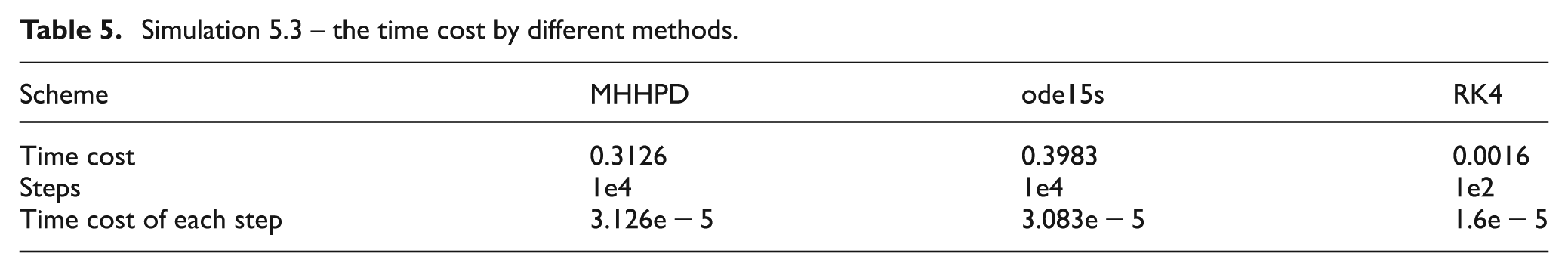
We set T = 2 s, N = 25, in the computation (cf. Algorithm 2). Owing to no exact solution for this complex structure problem, we compute a reference solution with a sufficiently small uniform time step size. Then, we compute the numerical solution using Algorithm 2, and we compare to Wilson θ (θ = 1.4) and Newmark β method (α = 0.25, β = 0.5) with uniform time step size k = 1/N∗, which is shown in Figure 6. In Figure 7, we show the scaling deformation and the deformation value at time T = 2 s. From Figures 6 and 7, we can see that Algorithm 2 is very efficient in the Pratt truss problem. Table 5 shows that MHHPD costs less than traditional methods.

Example 5.4 – numerical solutions with different method at Point 9.

Example 5.4 – the scaling deformation of the Pratt truss at T = 2 s.
Simulation 5.3 – the time cost by different methods.
Conclusion
In this article, a MHHPD is designed for solving time-varying nonhomogeneous systems. The time-varying problems with nonhomogeneous terms cannot be implemented with high precision; however, by introducing new variables twice, we can easily deal with this problem. MHHPD inherits the advantages of HPD method, which is an explicit method. For some problems, even though some extra variables are introduced and the dimensions are expanded, the proposed method is much more effective than some traditional methods.
In subsection ‘Convergence’, the convergency is given and subsection ‘Efficiency analysis’ shows the efficiency of MHHPD method. The influence of parameters is discussed in ‘Numerical simulations’, ‘A first-order time-varying nonhomogeneous system’ and ‘A nonhomogeneous Hermite equation’; the effectiveness for stiff problem ‘A time-varying nonhomogeneous system with multi-frequency’ and ‘A nonhomogeneous Hermite equation’ is demonstrated, and the application in engineering is also shown in ‘Engineering application’.
Numerical results show that the proposed method indeed provide solutions with high precision.
Footnotes
Handling Editor: Chenguang Yang
Declaration of conflicting interests
The author(s) declared no potential conflicts of interest with respect to the research, authorship, and/or publication of this article.
Funding
The author(s) disclosed receipt of the following financial support for the research, authorship, and/or publication of this article: This work was supported by the NSFC (grant no. 50876066), SSPU fund project (no.EGD15XQD14), Shanghai University Youth Teacher Training Program (no. ZZZZEGD15007) and SSPU Applied Mathematics key discipline (no. XXKPY1604).