Novel method to integrate MARG and an odometer into AHRS for moving vehicles

Abstract

To improve the performance of attitude and heading reference systems for moving vehicles, an effective orientation estimation method is proposed. The method involves the use of a low-cost magnetic, angular rate, and gravity sensor and an odometer. This study addresses the problems of large and abrupt changes in acceleration by moving vehicles and the issue of obtaining precise, long-term, drift-free attitude estimates. A low-pass filter is used to eliminate the high-frequency part of linear acceleration. An improved method to evaluate motion status is proposed and utilized to compensate for filtered accelerometer measurement when the vehicle is accelerating or steering. The proposed method uses an effective adaptive Kalman filter based on the error state model to reduce dynamic perturbations. Filter gain is adaptively tuned under different moving modes by adjusting the noise matrix. Experiments are performed to validate the algorithms under realistic motions, and simulations are implemented to examine their performance.

Introduction

Attitude estimation plays significant roles in the development of autonomous land vehicles for trajectory control and autonomous navigation applications.^1,2 Traditional orientation estimation methods are mainly based on infrared, radar, and video motion-sensing technologies, which can provide high system accuracy. ³ These techniques are costly and difficult to apply in land vehicles. The inertial/magnetic sensor is a self-contained and effective instrument that can be applied in unconstrained environments and moving cases; it does not require external sources. ⁴

The magnetic, angular rate, and gravity (MARG) sensor, a typical inertial/magnetic sensor module, contains a three-axis accelerometer, gyroscope, and magnetometer. ⁵ The angular rate of the gyroscope can be numerically integrated to determine the orientation, which presents a linear drift error after a long period of integration. The accelerometer and magnetometer measure the gravity and local magnetic field in the local coordinate system of the sensor; the two reference vectors are required to define the orientation. Pitch and roll angles are estimated with the gravity components of the accelerometer measurements, and the yaw angle is estimated by magnetometers. ⁶ This method is simple and drift-free but is not ideal for dynamic motions because the accelerometer measurements contain non-gravitational acceleration.^7,8 In addition, the magnetometer output can be affected by ferrous materials (e.g. the vehicle itself) near the sensor and magnetic field in the environment. The attitude and heading reference system (AHRS) based on the MARG sensor requires combining information from all the sensors to enhance accuracy.^9,10

Extensive research has been performed on the process of combining the two measurements to obtain accurate orientation estimation. The Kalman filter is considered an effective method, and different fusion methods based on this filter have been extensively discussed. Three key issues are encountered in the implementation of the fusion algorithm.

The first issue is building kinematic and measurement models based on different mathematical representations, which are used to define the rotation relationship between the body and the global reference frame, such as the Euler angle,^11–13 quaternion,^5,14 and the direction cosine matrix (DCM).^15,16 The Euler angle is the most calculation-efficient method to define the rotation matrix, but it is restricted to singularity problems when the pitch angle passes through the boundary condition (±π/2). In addition, the traditional Euler angle–based model is highly nonlinear because trigonometric and inverse trigonometric functions exist in the kinematics model. ⁹ This nonlinearity problem causes not only high computational costs but also system noise. The quaternion is widely used to avoid singularity; however, the nonlinearity problem still exists. To address the nonlinearity problem, the extended Kalman filter (EKF), which is the standard method for nonlinear attitude estimation, was introduced. ⁵ However, the method requires much computational time and still results in linearization errors compared with the regular Kalman filter. ¹⁷ The Kalman filter based on the DCM method avoids singularity and nonlinearity and exerts a better effect than EKF based on Euler and quaternion. ¹⁶ However, the method complicates the calculation because nine parameters, which are orthogonally constrained, need to be identified. ¹⁸

The second issue is dealing with the disturbance of linear acceleration and ferrous materials. Extensive research has been performed on orientation estimation for moving objects. Foxlin ¹⁹ designed a complementary separate-bias Kalman filter and comprehensively discussed the process setting and measurement noise covariance matrix under dynamic motion. Lee and Park ²⁰ proposed a minimum-order Kalman filter. They divided motion conditions into four cases, and a vector selector was used to handle various conditions. Yun et al. ²¹ proposed an adaptive-gain complementary filter to estimate the orientation of foot movement during both static and dynamic motions. They used a variable scalar gain factor to combine low-frequency measurements from the accelerometer and magnetometer and high-frequency measurements from the gyroscope. However, these studies were based on the specific assumption that movement pertains to the slow-motion condition. In other words, disturbance from linear acceleration and ferrous materials do not always exist. Although these methods have been effectively implemented in several specific applications, such as human body tracking, they are unsuitable for moving vehicles because of the long-time movement and extremely large linear acceleration.

The last issue is judging motion status under different conditions. A dynamic scalar defined as $\alpha =|\left|{\mathrm{f}}_{\mathrm{b}}\right|-\left|{\mathrm{g}}_{\mathrm{b}}\right||$ is utilized to judge the moving state, which is divided into three different modes. ²² However, the equation $\alpha =0$ does not prove that the two vectors are similar, which means that the vehicle is static or moving at a constant speed. For example, when the gravity-induced acceleration vector in the body frame is $\left[\begin{array}{ccc}0\hfill & 0.5\hfill & \sqrt{{\mathrm{g}}_0^2-{0.5}^2}\hfill \end{array}\right]$ and the vehicle is decelerating at 1 m/s² in the forward direction (Y-axis), the dynamic scalar is zero, but the vehicle is decelerating. A time threshold is added to avoid false triggers, ²³ and a walking robot is assumed to have no acceleration for a while after a few seconds of dynamic motion. However, this double-standard detection is unsuitable for moving vehicles because of the long-time movement.

In this study, a new method is proposed for low-cost AHRS. This method provides the following contributions to improve performance estimation:

1. The characteristics of movement noise are analyzed through numerical experiments. Linear acceleration is divided into two parts, and a low-pass filter is developed to eliminate the high-frequency part of linear acceleration.

2. A new method is proposed to identify the movement status and partly eliminate the low-frequency part of residual linear acceleration.

3. An adaptive Kalman filter (AKF) is developed for dynamic measurement. The singularity problem occurs in various applications, such as robotics, physical medicine, and airborne vehicles, but does not occur in land vehicles.^24,25 Therefore, the error state model based on the Euler angle is adopted. This model prevents the nonlinearity problem. ²² Through movement status identification and compensation, noise covariance matrices Q and R are specified.

A schematic of the system is shown in Figure 1. The rest of this article is organized as follows. The proposed method, including the orientation estimation algorithm, motion status determination, low-pass filter and compensation, and the linear Kalman filter, is described in section “Proposed approach.” Performance evaluation is conducted in sections “Experimental results” and “Simulation results” through a series of experiments and simulation. The conclusion is provided in section “Conclusion.”

Figure 1.

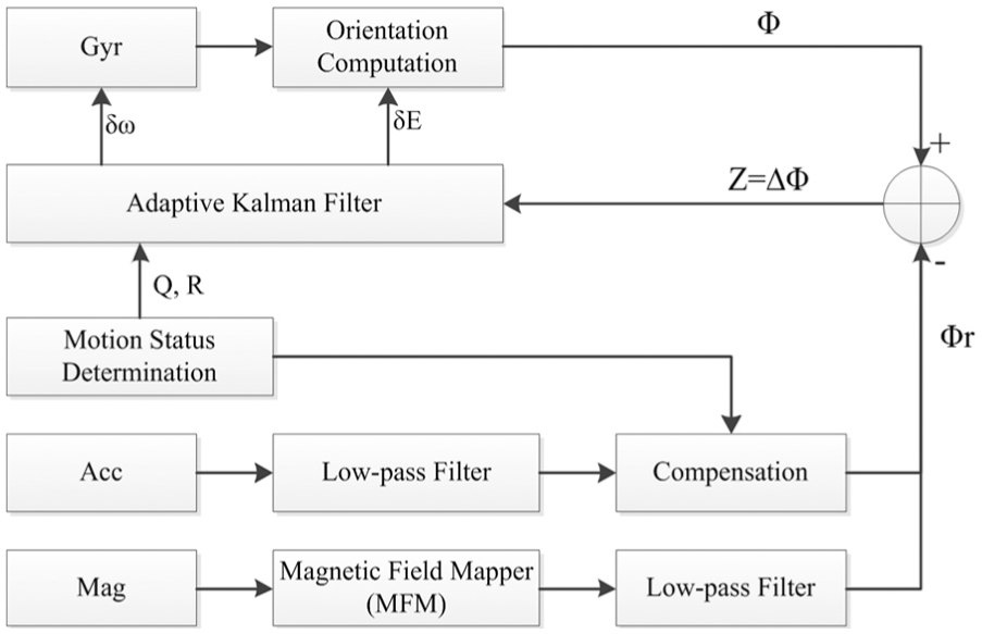
Schematic AHRS integrated with MARG and an odometer.

Proposed approach

Orientation estimation algorithm

AHRS determines orientation angles, which are also called Euler angles, including yaw $\phi$ , pitch $\gamma$ , and roll $\theta$ . Euler angles are defined as rotation angles from the body frame (b frame) to the navigation frame (n frame). MARG is assigned with a single coordinate system, which is synonymous to the body (or vehicle) coordinate system in this study, as shown in Figure 2. In Figure 2, the Y-axis is the moving direction, and the inertial navigation coordinate frame (n frame) comprises the east, north, and up frames.

Figure 2.

Navigation and body frame coordinate systems.

We let ${\mathrm{m}}_{\mathrm{b}}={[{\mathrm{m}}_{\mathrm{bx}}{\mathrm{m}}_{\mathrm{by}}{\mathrm{m}}_{\mathrm{bz}}]}^{\mathrm{T}}$ and ${\mathrm{G}}_{\mathrm{b}}=[{\mathrm{G}}_{\mathrm{bx}}{\mathrm{G}}_{\mathrm{by}}{\mathrm{G}}_{\mathrm{bz}}{]}^{\mathrm{T}}$ represent the projection vectors of the magnetic and gravity field reference vectors on the body frame. When no interference by linear acceleration and ferrous materials exists, the two vectors are equal to the magnetometer and accelerometer measurements.

The equations to estimate vehicle pitch and roll angles are as follows

$$\gamma =\mathrm{arctg}\left(\frac{{\mathrm{g}}_{\mathrm{by}}}{{\mathrm{g}}_{\mathrm{bz}}}\right)$$

(1)

$$\theta =\arcsin \left(\frac{{\mathrm{g}}_{\mathrm{bx}}}{\left|{\mathrm{g}}_{\mathrm{b}}\right|}\right)$$

(2)

Given the actual situation of the vehicle, only the pitch and roll angles within the range of [−π/4, π/4] are considered.

Using pitch $\gamma$ and roll $\theta$ derived by accelerometer measurements, we define

$$\phi =\mathrm{arctg}\left(\frac{{\mathrm{m}}_{\mathrm{bz}}\sin \gamma -{\mathrm{m}}_{\mathrm{by}}\cos \gamma }{{\mathrm{m}}_{\mathrm{bx}}\cos \theta +({\mathrm{m}}_{\mathrm{by}}\sin \gamma +{\mathrm{m}}_{\mathrm{bz}}\cos \gamma )\sin \theta }\right)$$

(3)

Motion of a vehicle on a road surface

The three-axis accelerometer affixed to the orthogonal axes of a moving vehicle measures the total acceleration, which consists of gravity-induced acceleration (gravity field on the body frame) and translational linear acceleration. To address the problem of attitude estimation under acceleration, distinguishing gravity-induced acceleration from acceleration measurements is important.

Unlike in the case of an aircraft, the motion of a land vehicle on a road is governed by two nonholonomic constraints. ² Except in special cases, such as sliding and jumping off the ground, the X-axis and Z-axis direction velocities of the vehicle on the road are considered zero. Similarly, the linear accelerations of the vehicle are zero under ideal conditions. The linear acceleration of the vehicle is mainly caused by accelerating (or decelerating) and turning. In this study, the vehicle state is divided into four modes as follows: stationary, low acceleration, accelerating, and steering.

In the stationary mode (Case 1), the vehicle is regarded as not moving rather than having no linear acceleration. Although the two conditions are similar in terms of the calculation of attitude, determining whether the moment linear acceleration is zero is difficult. In the low-acceleration mode (Case 2), the vehicle is running at a nearly constant speed. In this case, the magnitude of accelerometer noise is generally small. However, sometimes the magnitude is extremely large (up to 2 m/s²) and presents high frequency. Vehicle motions in the accelerating (Case 3) and steering (Case 4) modes are collectively summarized as the high-acceleration mode. According to Newton’s law, accelerating motion requires longitudinal (Y-axis) linear acceleration, whereas steering motion requires transverse (X-axis) linear acceleration.

In consideration of driver comfort, the attitude variation in the vehicle is not drastic, which means gravity-induced acceleration has low frequency. Although the frequency characteristic of the high-acceleration mode is complicated, the acceleration can be roughly divided into high frequency and low frequency, as shown in equation (4)

$${\mathrm{f}}_{\mathrm{b}}={\mathrm{f}}_{\mathrm{bH}}+{\mathrm{f}}_{\mathrm{bL}}$$

(4)

Based on these analyses, a low-pass filter is used to eliminate the high-frequency part of linear acceleration. This process is called the first-step process to the signal. The accelerometer measurement consists of the gravity-induced acceleration and the low-frequency part of linear acceleration.

Motion status determination

The disadvantages of traditional discriminant methods were discussed in the previous sections. In this section, an odometer and a gyroscope work together to determine the motion status and eliminate linear acceleration. As a cost-effective and requisite sensor for land vehicles, the odometer measures the incremental distance and forward direction velocity along the vehicle trajectory. The odometer is a reliable sensor for benign surfaces and presents good stability independent of running time. Y-axis linear acceleration is used to determine whether the vehicle is accelerating, which can be obtained through the differential of the forward direction velocity. The gyroscope provides angular rate ${\omega }_{\mathrm{z}}$ around the Z-axis, which indicates when the vehicle is turning. The criteria of the different motion statuses are shown in Table 1. The X- and Y-axes linear accelerations can be calculated as

$${\mathrm{a}}_{\mathrm{cy}}=\frac{\mathrm{d}{\mathrm{V}}_{\mathrm{od}}}{\mathrm{dt}}$$

(5)

$${\mathrm{a}}_{\mathrm{cx}}={\omega }_{\mathrm{z}}{\mathrm{V}}_{\mathrm{od}}$$

(6)

where ${\mathrm{V}}_{\mathrm{od}}$ is the forward direction velocity from the odometer and ${\mathrm{a}}_{\mathrm{c}}=\left[\begin{array}{cc}{\mathrm{a}}_{\mathrm{cx}}\hfill & {\mathrm{a}}_{\mathrm{cy}}\hfill \end{array}\right]$ is the estimation of linear acceleration ${\mathrm{a}}_{\mathrm{b}}$ in X- and Y-axes.

Table 1.

Criteria of different motion statuses.

	Case 1	Case 2	Case 3	Case 4
Criteria	${\mathrm{V}}_{\mathrm{od}}=0$	${\mathrm{a}}_{\mathrm{cy}}\le \mathrm{T}{\mathrm{h}}_1,{\mathrm{a}}_{\mathrm{cx}}\le \mathrm{T}{\mathrm{h}}_2$	${\mathrm{a}}_{\mathrm{cy}}>\mathrm{T}{\mathrm{h}}_1$	${\mathrm{a}}_{\mathrm{cx}}>\mathrm{T}{\mathrm{h}}_2$

The forward velocity provided by the odometer is calculated by dividing incremental distance $\mathrm{d}{\mathrm{S}}_{\mathrm{od}}$ by sampling time $\mathrm{dt}$ , as shown in the following

$${\mathrm{V}}_{\mathrm{od}}=\frac{\mathrm{d}{\mathrm{S}}_{\mathrm{od}}}{\mathrm{dt}}$$

(7)

After one to two differential calculations, the calculated acceleration ${\mathrm{a}}_{\mathrm{c}}$ is closer to the low-frequency part of acceleration ${\mathrm{f}}_{\mathrm{bL}}$ than to instantaneous acceleration ${\mathrm{f}}_{\mathrm{b}}$ . Given the small delay of the low-pass filter and the difference in sampling frequency, the calculated acceleration ${\mathrm{a}}_{\mathrm{c}}$ cannot be completely equal to ${\mathrm{f}}_{\mathrm{bL}}$ unless the acceleration is constant. Therefore, a diminutive compensation for acceleration is provided by two scale factors ${\mathrm{k}}_1$ and ${\mathrm{k}}_2$ . Then, an estimate of gravity-induced acceleration ${\mathrm{G}}_{\mathrm{c}}$ can be calculated with equations (8)–(10)

$${\mathrm{G}}_{\mathrm{cz}}={\mathrm{f}}_{\mathrm{bLz}}$$

(8)

$${\mathrm{G}}_{\mathrm{cy}}=\{\begin{array}{c}{\mathrm{f}}_{\mathrm{bLy}}-{\mathrm{k}}_1{\mathrm{a}}_{\mathrm{cy}}\hfill \\ \multicolumn{1}{c}{{\mathrm{f}}_{\mathrm{bLy}}}\end{array}\begin{array}{c}\mathrm{Case}3\hfill \\ \multicolumn{1}{c}{\mathrm{otherwise}}\end{array}$$

(9)

$${\mathrm{G}}_{\mathrm{cx}}=\{\begin{array}{c}{\mathrm{f}}_{\mathrm{bLx}}-{\mathrm{k}}_2{\mathrm{a}}_{\mathrm{cx}}\hfill \\ \multicolumn{1}{c}{{\mathrm{f}}_{\mathrm{bLx}}}\end{array}\begin{array}{c}\mathrm{Case}4\hfill \\ \multicolumn{1}{c}{\mathrm{otherwise}}\end{array}$$

(10)

Implementation of linear Kalman filter

The first step in designing a Kalman filter for orientation estimation is to determine the components of the state and measurement vectors. Given that the basic purpose of the Kalman filter is to estimate orientation, most references directly included the state variables of orientation or its substitutes (e.g. quaternion) in the state vector, which will lead to nonlinearity and singularity problems. In this section, a linear kinematic model is proposed based on the error state model. Given that the purpose of the Kalman filter is to estimate orientation and gyro drift over time, the state vector is designed as

$$\mathrm{X}={\left[\begin{array}{cc}\delta \mathrm{E}\hfill & \delta \omega \hfill \end{array}\right]}^{\mathrm{T}}$$

(11)

where $\delta \mathrm{E}$ is the three-axis small-angle rotation error vector and $\delta \omega$ is the three-axis gyro bias vector. The observation vector is constructed as

$$\mathrm{Z}={\left[\begin{array}{ccc}\delta \gamma \hfill & \delta \theta \hfill & \delta \phi \hfill \end{array}\right]}^{\mathrm{T}}$$

(12)

where $\delta \gamma \mathrm{and}\mathrm{\delta }\mathrm{\theta }$ are elements of the Euler angle deviation vector between the accelerometer and update and $\delta \phi$ is the heading residual between the magnetometer and update. ¹⁷ The dynamic and observation models are expressed as

$$\stackrel{·}{\mathrm{X}}=\mathrm{DX}+\mathrm{w}=\left[\begin{array}{c}\begin{array}{cc}{\omega }_{\mathrm{in}}^{\mathrm{n}}\times \hfill & -{\mathrm{C}}_{\mathrm{b}}^{\mathrm{n}}\hfill \end{array}\hfill \\ \multicolumn{1}{c}{0_{3\times 6}}\end{array}\right]\mathrm{X}+\mathrm{w}$$

(13)

$$\mathrm{Z}=\mathrm{HX}+\mathrm{v}=\left[\begin{array}{cc}{\mathrm{I}}_3\hfill & 0_3\hfill \end{array}\right]\mathrm{X}+\mathrm{v}$$

(14)

where process noise vectors $\mathrm{w}$ and $\mathrm{v}$ are independent Gaussian white noises with a zero mean

$$\mathrm{w}~\mathrm{N}(0,\mathrm{Q})$$

(15)

$$\mathrm{v}~\mathrm{N}(0,\mathrm{R})$$

(16)

where $\mathrm{Q}$ and $\mathrm{R}$ are the process and measurement noise covariance matrices, respectively.

Noise covariance matrices $\mathrm{Q}$ and $\mathrm{R}$

The main obstacle in applying the Kalman filter is specifying covariance matrices $\mathrm{Q}$ and $\mathrm{R}$ . In this section, the covariance matrices are approximated under different conditions. All the sensors are assumed to have been calibrated for axis alignment and direct current (DC) bias. Process noise covariance matrix $\mathrm{Q}$ can be determined through spectral density analysis of the process noise of the gyroscope and its associated drift. ²² We set

$$\mathrm{Q}=\left[\begin{array}{cc}{\mathrm{Q}}_{\mathrm{w}}\hfill & 0\hfill \\ \multicolumn{1}{c}{0}& {\mathrm{Q}}_{\mathrm{b}}\hfill \end{array}\right]$$

(17)

where ${\mathrm{Q}}_{\mathrm{b}}$ is the three-order matrix of the gyro bias driven by the rate random walk process and ${\mathrm{Q}}_{\mathrm{w}}$ is a three-order diagonal matrix that is entirely caused by the noise floor of the gyro. Based on equation (13), ${\mathrm{Q}}_{\mathrm{w}}$ is expressed as ¹⁹

$${\mathrm{Q}}_{\mathrm{w}}=\left[\begin{array}{ccc}{\sigma }_{\mathrm{x}}^2\hfill & 0\hfill & 0\hfill \\ \multicolumn{1}{c}{0}& {\sigma }_{\mathrm{y}}^2\hfill & 0\hfill \\ \multicolumn{1}{c}{0}& 0\hfill & {\sigma }_{\mathrm{z}}^2\hfill \end{array}\right]$$

(18)

$${\sigma }_{\mathrm{i}}={\sigma }_0\Delta \mathrm{t}(1+{\omega }_{\mathrm{i}}^2)\mathrm{i}=\mathrm{x},\mathrm{y},\mathrm{z}$$

(19)

where ${\sigma }_0$ is the gyroscope bias stability and $\Delta \mathrm{t}$ is the discrete time.

Matrix $\mathrm{R}$ represents measurement noise, which is difficult to determine because it is extremely nonwhite. ¹⁹ The major source of the measurement noise of the pitch and roll angles is linear acceleration, which is divided into high- and low-frequency parts, as shown in equation (4). With a low-pass filter and acceleration compensations, measurement noise is considerably reduced and determined by the estimation error after treatment. The noise of the high-frequency part is determined by the effect of the low-pass filter, especially the cutoff frequency of the filter. The noise of the low-frequency part refers to the compensation error in this study, which is related to the magnitude of linear acceleration, given that this compensation is partial. These two parts of noise, total as ${\sigma }_{\gamma 0}^2$ , need not be considered in Case 1, in which the major measurement noise ${\sigma }_{\mathrm{v}}^2$ is decided by the accelerometer scale error. Notably, the scale error of the accelerometer is smaller than those of the other parts of noise.

The calculations of the two angles are completely independent (shown as equations (1) and (2)), ²² and the noise of the angles is handled differently in different cases. During vehicle motions in Case 3 or Case 4, an additive function noise^6,23 is adopted to increase the accelerometer noise proportionally to the increments of the linear acceleration. Then, the influence of accelerometer corrections will be decreased. The additive function noises of pitch and roll angles are formed as ${\mathrm{k}}_3{\mathrm{a}}_{\mathrm{cy}}^2$ (Case 3) and ${\mathrm{k}}_4{\mathrm{a}}_{\mathrm{cx}}^2$ (Case 4).

The magnetometer is disturbed by the magnetic field in the environment. Magnetic interference results from the vehicle itself and the surrounding objects. A calibration procedure based on the ellipse-specific fitting error compensation method is executed on the magnetometer to remove the influence of the vehicle. In practical applications, a MARG-inside vehicle cannot be calibrated perfectly because the calibration process requires a constant-speed rotational motion and a large number of data samples distributed in a unit sphere. The calibration error ${\sigma }_{\phi 0}^2$ is considered in the calculation of the yaw angle. The magnetic effect from the surrounding objects is not discussed in this article.

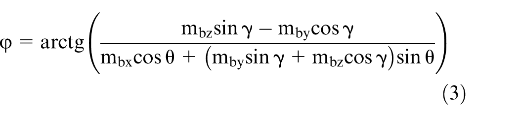
In addition, as shown in equation (3), the calculation of the yaw angle depends largely on the exact calculation of the inclination angle (pitch and roll angles). To include this influence, this additive function noise is formed as ${\mathrm{k}}_5{\max \{\mathrm{\sigma }}_{\gamma }^2,{\sigma }_{\theta }^2\}$ in equation (23).

Based on these analyses, the algorithm used to set $\mathrm{R}$ is

$$\mathrm{R}=\left[\begin{array}{ccc}{\sigma }_{\gamma }^2\hfill & 0\hfill & 0\hfill \\ \multicolumn{1}{c}{0}& {\sigma }_{\theta }^2\hfill & 0\hfill \\ \multicolumn{1}{c}{0}& 0\hfill & {\sigma }_{\phi }^2\hfill \end{array}\right]$$

(20)

where

$${\sigma }_{\gamma }^2={\mathrm{k}}_3{\mathrm{a}}_{\mathrm{cy}}^2+{\sigma }_{\gamma 0}^2(1-\mathrm{m})+{\sigma }_{\mathrm{v}}^2$$

(21)

$${\sigma }_{\theta }^2={\mathrm{k}}_4{\mathrm{a}}_{\mathrm{cx}}^2+{\sigma }_{\theta 0}^2(1-\mathrm{m})+{\sigma }_{\mathrm{v}}^2$$

(22)

$${\sigma }_{\phi }^2={\mathrm{k}}_5{\max \{\mathrm{\sigma }}_{\gamma }^2,{\sigma }_{\theta }^2\}+{\sigma }_{\phi 0}^2$$

(23)

where $\mathrm{m}=\{\begin{array}{c}1\hfill \\ \multicolumn{1}{c}{0}\end{array}\begin{array}{c}\mathrm{case}1\hfill \\ \multicolumn{1}{c}{\mathrm{otherwise}}\end{array}$ , ${\sigma }_{\phi 0}^2$ is the noise covariance of the calibration error, and the scale parameter ${\mathrm{k}}_{\mathrm{i}}(\mathrm{i}=3,4,5)$ can be determined by the design requirements and experiments.

Experimental results

Experimental setup

Two MTi MARG sensors were used to record the experimental data and verify the proposed algorithm. The MTi sensor can output both Euler angles using its algorithm and raw sensor data, including the calibrated three-axis acceleration, rate of turn (gyro), and magnetic field. MTi-30 is a low-cost MARG sensor, and its specifications are shown in Table 2. The expected accuracy of roll and pitch is 0.4° when static and 1.0° when dynamic (1σ root mean square (RMS)). In a homogenous magnetic field, the accuracy of yaw is 1.0°. MTi-G-700 consists of high-precision sensors and an additional GPS and provides higher accuracy of attitude measurement than the MTi-30 MARG sensor. In this study, MTi-G-700 data were used to compare and verify the effectiveness of the low-pass filter and the compensation in section “Low-pass filter and compensation.” MTi was fixed on an experimental car. In section “Low-pass filter and compensation,” the attitude estimation from MTi-G-700 is considered sufficiently accurate for comparison. MARG sensor data (including all the above-mentioned driving conditions except for Case 1) were collected at a sampling rate of 100 Hz as the test car drove along. The trajectory is shown in Figure 3.

Table 2.

Specifications of the MTi-30 sensor.

Parameter (unit)	Value
Gyroscope noise density ( $\circ /\mathrm{s}/\sqrt{\mathrm{Hz}}$ )	0.03
Gyroscope bias stability ( $\circ /\mathrm{h}$ )	18
Accelerometer noise density ( $\mathrm{\mu }\mathrm{g}/\sqrt{\mathrm{Hz}}$ )	80
Accelerometer bias stability ( $\mathrm{m}/{\mathrm{s}}^2$ )	0.03
Magnetometer noise density ( $\mathrm{m}\mathrm{Gauss}/\sqrt{\mathrm{Hz}}$ )	200

Figure 3.

Trajectory of the experiment.

Low-pass filter and compensation

Numerical experiments were conducted to demonstrate the effectiveness of the low-pass filter. These experiments considered daily driving conditions, including accelerating, turning, waiting for the traffic light to change, and driving on a hill. The gravity-induced and linear acceleration vectors were calculated with the accelerometer signals, and the Euler angles were calculated with MTi-G-700. MTi-G-700 data were used for comparison. All sensor data were logged and processed in MATLAB.

The experiment lasted approximately 10 min with a sampling rate of 100 Hz. A total of 60,123 data samples were collected. Fast Fourier transformation (FFT) was performed on the two calculated vectors to analyze their frequency characteristics. Figure 4 shows the frequency characteristics of the two acceleration vectors. The low-frequency characteristic of gravity-induced acceleration, which is equal to the characteristics of the Euler angles of a vehicle, proves that the low-pass filter can be used to remove the high-frequency part of linear acceleration. The cutoff frequency of the low-pass filter was set to $\mathrm{CF}=[5\mathrm{Hz},5\mathrm{Hz},\mathrm{and}3\mathrm{Hz}]$ (for X-, Y-, and Z-axes, respectively), and the filter was completed in MATLAB.

Figure 4.

Frequency characteristics of linear acceleration and the gravity field: (a) FFT of the gravity field and (b) FFT of linear acceleration.

The effect of the low-pass filter is shown in Figure 5, in which the red, blue, and black lines represent the accelerometer measurements before and after the filter was applied. Gravity-induced acceleration was calculated by MTi-G-700. Figure 5 shows only a short-period (e.g. from 100 to 105 s) comparison to avoid presenting an extremely dense curve. The magnitude of the high-frequency part of linear acceleration noise is generally extremely large (up to 1 m/s²). The comparison shows that the low-pass filter eliminated most of the high-frequency movement noises, and the accelerometer signals after filtering are smooth and close to the gravity-induced accelerations. Although the low-pass filter could not completely eliminate the linear accelerations, especially the low-frequency part, the method can still be used to provide compensation.

Figure 5.

Gravity vector and accelerometer measurements before and after filtering.

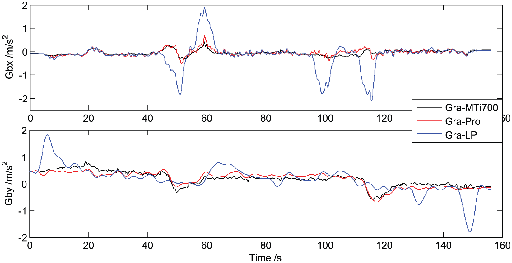
The compensation effect of the proposed method on linear acceleration was also studied. Figure 6 shows the experimental results of linear acceleration estimation by MTi-G-700 and the proposed method using an odometer. In the test, the magnitude of the low-frequency part of linear acceleration sometimes reached 2 m/s². Figure 6(b) and (d) shows the comparison results of X-axis and Y-axis linear accelerations after low-pass filtering. The proposed method can effectively estimate the linear acceleration of the low-frequency part, but not entirely. If the filtering process of the last step is not implemented, estimating and compensating for linear acceleration would be difficult because of the chaotic noise of all the sensors, as shown in Figure 6(a) and (c). Given that the linear acceleration of the Y-axis was calculated by differential calculus in equation (16) and that the calculation frequency was sufficiently high, the results are much worse than that in the X direction. After low-pass filtering and compensation, gravity-induced acceleration was estimated with equations (8)–(10). The values of scale factors ${\mathrm{k}}_1=0.92$ and ${\mathrm{k}}_2=0.85$ were finalized to reduce the maximum estimation error. Figure 7 shows the estimation results of gravity-induced acceleration by MTi-G-700, by the proposed method, and the initial data using low-pass filtering only. After the compensation, the maximum estimation error decreased from 2.04 to 0.36 m/s² on the X-axis and from 1.67 to 0.38 m/s² on the Y-axis. Inspection of the plot shows that the difference among the three estimations is small in case 2, especially on the X-axis, and the estimation using the proposed method is not completely accurate on the Y-axis. Therefore, compensation in case 2 is no longer required. The switch threshold was determined to analyze the estimation accuracy of the proposed method: $\mathrm{T}{\mathrm{h}}_1=0.25$ and $\mathrm{T}{\mathrm{h}}_2=0.15$ . Based on the maximum error produced by the threshold, noise covariance functions ${\sigma }_{\gamma 0}^2=0.{015}^2$ and ${\sigma }_{\theta 0}^2=0.{025}^2$ were determined.

Figure 6.

Experimental results of linear acceleration estimation by MTi-G-700 and the proposed method using an odometer: (a and c) estimations before low-pass filtering and (b and d) estimations after low-pass filtering.

Figure 7.

Estimation results of gravity-induced acceleration. The black, red, and blue curves are the outputs of MTi-G-700, proposed method, and low-pass filtering only, respectively.

Magnetometer calibration

When a magnetometer is mounted on an object (vehicle) that contains ferromagnetic materials, the measured (Earth) magnetic field is distorted and causes an error in the measured orientation. However, the disturbance of the magnetic field can be corrected by applying a specialized calibration procedure. ²⁶ Accurate calibration is obtained by recording MARG signals while rotating the object in a space without nearby ferromagnetic materials. The software kit of the MTi sensor provides a calibration procedure called Magnetic Field Mapper (MFM). When the object is rotated by a sufficiently large number of orientations, MFM can calculate new calibration parameters that can be immediately used in MTi-30.

In a non-disturbed magnetic field, the 3D measured magnetic field vector has a magnitude of 1; therefore, all measured points lie on the circumference of a sphere with the center at zero. In a disturbed magnetic field, this sphere is both shifted and warped. The calibration procedure based on the ellipse-specific fitting error compensation method aims to produce a function that maps the measured magnetic field vector to a sphere. The calibration procedure requires inclination. The accuracy of inclination is influenced by linear accelerations. Large accelerations significantly affect the accuracy of the calibration results. In addition, the calibration procedure works best if the object is rotated by a large number of possible orientations. To achieve ideal results, the vehicle is driven at a steady speed of below 0.5 m/s² for about 2 min.

The calibration results of the magnetometer show that MFM was able to apply the new magnetic field model to all corrected magnetic field measurements of the file or measurement in Figure 8. The norm of the magnetic field vector corresponding to each sampling point is shown in Figure 8(a). The flatter the blue line is (and the closer to 1.0 it is), the better the magnetic mapping is. Compared with the raw data outputs before MFM, a significant amount of interference was well compensated. Figure 8(b) shows the difference among all the values in all directions after calibration. According to equation (3), we set ${\sigma }_{\phi 0}^2=0.2^2$ in this experiment.

Figure 8.

Calibration results of the magnetometer: (a) norm of the magnetic field before (red line) and after (blue line) magnetic field mapping and (b) difference in all directions after calibration. The red, blue, and green curves are the outputs of the X-, Y-, and Z-axes.

Orientation estimation results

The same experiment with real land vehicles was performed again, as shown in Figure 3, and the data were logged by the MTi-30 MARG sensor. The experiment lasted for 154 s at a sampling rate of 100 Hz. The attitude estimations by MTi, gyro only, and the proposed method were compared, as shown in Figure 9. When the gyro-only method was used, the estimation error increased over time, and a large drift was observed after a few seconds. This drift obviously existed when turning (e.g. 110–120 s). The Euler angles of the proposed method and MTi are almost the same. Evidently, the proposed filter can eliminate long-term drift through real-time gyro error estimation and compensation.

Figure 9.

Orientation estimation results of the experimental vehicle.

Setting the output of MTi as the real results, the attitude errors of estimated gravity vector, gyro only, and the proposed method were plotted in Figure 10. It shows that the disturbance of linear acceleration and the drift error are solved by the proposed method. The error analysis was shown in Table 3, and the results show that accuracy of the proposed method is within 1.5°.

Figure 10.

Orientation estimation error results of different methods. The black, blue, and red curves are the outputs of proposed method, gyroscope only, and estimated gravity vector, respectively.

Table 3.

Orientation estimation errors of the experiment.

	Pitch (°; RMS)	Roll (°; RMS)	Yaw (°; RMS)	Pitch (°; Max)	Roll (°; Max)	Yaw (°; Max)
Pro AKF	0.536	0.323	0.737	1.286	1.031	1.323
Gyration only	2.543	1.252	1.436	5.415	3.407	3.238
Gravity	0.817	0.462	None	2.529	2.205	None

To determine the accuracy of the proposed method and whether the proposed method presents better estimation performance than MTi-30 and the traditional AKF method, several simulations with the same noise characteristics as the experiment were implemented.

Simulation results

Given the limitations of experimental study, a comprehensive simulation study was implemented to examine the performance of the proposed estimation algorithm. Simulation performance is simultaneously affected by numerous factors, including magnetometer calibration errors, linear acceleration interference, and random measurement error, during actual experiments. The designed simulations considered these factors based on previous experiments and analyses. With these simulations, the effects of the process on filter performance can be individually analyzed. Additionally, the simulation provides an opportunity to compare the proposed method with other methods.

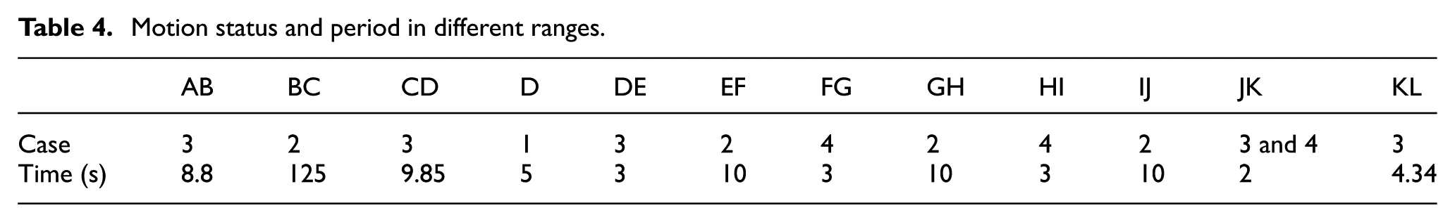
The simulation was designed to validate filter performance under an actual running state. This simulation has two objectives: verify if the algorithm can correct the orientation error when the vehicle is stationary (engine idling) (Ob1) and verify the reliability of the algorithm in long-term operation (Ob2). The movement route of the simulation vehicle is shown in Figure 11. Letters are used to indicate the different motion statuses shown in Table 4. For example, the vehicle is accelerating when it starts in AB, and it stops at the junction waiting for the semaphore in D.

Figure 11.

Movement route of the simulation vehicle. A different letter denotes the beginning of a different motion status, as shown in Table 3.

Table 4.

Motion status and period in different ranges.

	AB	BC	CD	D	DE	EF	FG	GH	HI	IJ	JK	KL
Case	3	2	3	1	3	2	4	2	4	2	3 and 4	3
Time (s)	8.8	125	9.85	5	3	10	3	10	3	10	2	4.34

The simulation considered the four main driving statuses mentioned above. MARG was assumed to be attached to the center of the vehicle, and the vehicle only rotates around the Z-axis. In the simulation, linear acceleration is modeled as

$${\mathrm{f}}_{\mathrm{b}}={\mathrm{a}}_{\mathrm{b}}+\mathrm{\sigma }\mathrm{randn}(*)$$

(24)

where $\mathrm{randn}(*)$ is the random number generator that produces samples with a Gaussian distribution ²¹ and σ is the standard deviation. Moreover, a rate gyro offset of 18°/h was added to ensure realistic simulations. Changing the value of ${\omega }_{\mathrm{z}}$ and ${\mathrm{a}}_{\mathrm{b}}$ can transform the movement status, where ${\mathrm{a}}_{\mathrm{by}}=1+\sin (0.4\pi \mathrm{t})\mathrm{m}/{\mathrm{s}}^2$ when accelerating ( ${\mathrm{a}}_{\mathrm{by}}=-1$ when decelerating), and ${\mathrm{a}}_{\mathrm{by}}=0$ in Case 2. The value of ${\omega }_{\mathrm{z}}$ is determined by turning speed and time. Standard deviation σ has different values in different cases and directions when compared with that in the previous experiment (from MTi-G-700). The modeling of the odometer was well illustrated by Wu et al. ²⁴ Each sensor measurement was added with white noise according to the accuracy of the sensor. The attitude estimation precision between the proposed method and the traditional AKF method without a low-pass filter and compensation was compared. The traditional AKF method was well introduced by Yun et al. ²¹ The actual attitude can be calculated by integrating angular velocity with respect to time. Therefore, estimation performance can be evaluated by computing the deviation between the estimated vector and the actual case.

Figure 12 shows the simulation speed of the vehicle in motion. Figure 12 shows a good simulation of these statuses, such as low-acceleration mode (Case 2) from 8.8 to 133.8 s. The estimation errors of ${\mathrm{G}}_{\mathrm{b}}$ (on X- and Y-axes) before and after the proposed process are shown in Figure 13. The errors between the actual gravity field and the raw data measured by the accelerometer are large and will directly lead to inaccurate observations. These errors can be significantly reduced by the proposed treatment.

Figure 12.

Simulation speed of the vehicle in motion.

Figure 13.

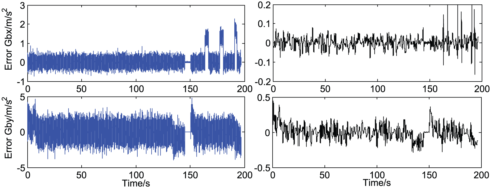
Estimation errors of ${\mathrm{G}}_{\mathrm{b}}$ before (left) and after (right) the proposed process.

The estimation results of the two methods are shown in Figure 14. With regard to Ob1, the standard deviation of stage D is [0.027°, 0.017°, 0.160°], whereas it is [0.260°, 0.583°, 0.660°] for traditional AKF attitude estimation. In the stationary mode (Case 1), the proposed method presented a good judgment performance, whereas the traditional AKF did not work well, as shown in Figure 15. Stage D refers to the state wherein the vehicle is static and the engine is still working. The effect of engine vibration caused the correction effect to be ineffective in the traditional AKF, whereas the low-pass filter provided a good elimination of this effect.

Figure 14.

Attitude estimation results of different filters.

Figure 15.

Estimation results of case number in stage D.

The simulation lasted for about 197 s, and the maximum estimation error of the proposed method was [0.690°, 0.340°, 0.722°] during this period. Compared with the maximum estimation error of [1.112°, 1.000°, 0.994°] in the traditional AKF, the proposed method presented better performance, especially in roll estimation. The improvement in estimating the yaw angle is due to the accurate estimation of pitch and roll. With regard to Ob2, the estimation error is stable and limited by the value calculated from the estimated gravity-induced acceleration. In addition, the correction in Case 1 can improve the stability of the algorithm.

Conclusion

A hybrid attitude estimation method was developed for moving vehicles. The method considers four different driving conditions and consists of three steps. First, a low-pass filter was used to eliminate high-frequency noise, which mainly originated from linear acceleration and resulted in flat accelerometer measurement curves. Second, a gyroscope and an odometer were combined to determine the moving state and estimate linear acceleration to provide a compensation for filtered accelerometer measurement when the vehicle is accelerating or steering. An AKF was also developed to adapt to the dynamic measurement. According to the evaluation of the moving state, the noise covariance matrix can be tuned adaptively to yield the optimal gain for ideal state estimation during dynamic periods. The experiments showed that the proposed method successfully eliminated long-term drift and maintained its stability indefinitely compared with the MTi outputs. The accuracy and superiority of the proposed method were fully demonstrated in the designed simulation. These results demonstrate that the proposed fusion algorithm can successfully deal with the integration errors of the gyroscope and linear acceleration interference.

For land vehicles, the magnetic interference from surrounding objects is significant but was not discussed in this article. Future research must consider this effect.