Evaluation of gas turbine diagnostic techniques under variable fault conditions

Abstract

The aim of this study is to evaluate gas path diagnostic techniques using a principle of variable structure classification applied to cover possible fault scenarios in gas turbine maintenance. This principle allows creating more versatile and realistic fault conditions relative to existing studies such as complex fault classifications, a new boundary for fault severity, and real deviation errors. The techniques analyzed are included into a special procedure that repeats a diagnostic process many times and computes for each fault class a probability of correct diagnosis. Using this probability averaged for all the classes as the evaluation criterion, the techniques are tested under the conditions of four comparative studies. The results show that (a) there is no single technique significantly outperforming all others over the full range of diagnostic conditions even if engine operating modes, fault simulation data, fault classifications, multiple-class boundaries or the scheme of deviation errors are varied; (b) the common level of diagnosis accuracy greatly depends on the fault classification used; (c) significant influence of fault severity boundary is found. The boundary proposed makes the level of accuracy much more realistic compared to simplified boundaries previously used; and (d) the use of real deviation noise in fault class description instead of simulated errors further approaches the diagnostic conditions and results to the level expected in practice.

Introduction

Important gas turbine aspects such as reliability, safety, maintenance, and operation costs are strongly affected by faults and deterioration. Condition-based maintenance and condition-monitoring systems help mitigate these problems. ¹ Diagnostic systems include different approaches such as thermography, boroscopy inspection, vibration and acoustic analysis, diagnostics of fuel and oil systems, wear debris analysis, and gas path analysis (GPA). This last approach has been widely used in the field of gas turbine monitoring. The systems based on GPA collect, filtrate, and intelligently analyze measured gas path variables to monitor the engine, identify incipient problems, and predict future changes. Over the past years, fault identification algorithms have been developed based on diverse pattern recognition and machine learning techniques.^2–5 Since gas turbines are very complex machines and need to be monitored, exhaustive comparative studies about diagnostic techniques can give clearer and more solid recommendations on how to construct an effective monitoring system.^3,4 Considering this necessity, this investigation evaluates two types of gas path diagnostic techniques: support vector machines (SVMs) and artificial neural networks (ANNs). The ANNs analyzed are multi-layer perceptron (MLP), radial basis network (RBN), and probabilistic neural network (PNN).

Different studies demonstrate that ANNs are outperformed by SVMs in many aspects.^6,7 Some of them are as follows: ANNs suffer from multiple local minima while the solution of SVMs is global and unique; ANNs are much more prone to overfitting than SVMs; SVMs have better generalization than ANNs for small number of samples; the geometric interpretation of SVMs is simpler and give sparse solutions; ANNs use empirical risk minimization, while SVMs use structural risk minimization; and unlike of SVMs, the computational complexity of ANNs directly depends on the input space dimensionality.

Despite the above explanations, the intention of the present diagnostic technique evaluation is to address other important issues in the field of gas turbine condition monitoring. First, the theoretical accuracy results provided by other studies are still not sufficient to give a clearer idea to designers, diagnosticians, and engineers on how accurate the diagnostic decisions will be for a wide range of gas turbine diagnostic conditions and how much these conditions affect the techniques employed. Second, the necessity of considering engine fault representations closer to reality is essential in order to produce more truthful and reliable diagnostic assessments.

For this purpose, this study proposes a principle of variable fault classification to study possible fault scenarios present in real gas turbine maintenance and create complex and realistic fault classifications. Through an adaptable algorithm, the variable classification makes it easy to determine the type of class used, different fault parameters, class quantity, fault development directions, fault severity boundary type, engine components and scheme of deviation noise. Based on this principle, 12 classifications of variations have been created for examining themselves and comparing the techniques. These classifications contain single or multiple classes as well as their mixtures. In addition, the study introduces and investigates a new boundary for fault severity. With this boundary, the fault class description becomes more realistic, thus providing more confidence to diagnosis results. This article also addresses the influence of real deviation errors on operation of diagnostic techniques and final diagnosis accuracy. A non-linear thermodynamic model of a stationary power plant for natural gas pipeline applications is used to construct the necessary fault classification.

A special procedure is developed to compare diagnostic techniques and compute the probability of correct diagnosis (true positive rate), which is used as the evaluation criterion. The described diagnostic technique evaluation procedure is implemented in MATLAB that offers convenient toolboxes for both machine learning and pattern recognition assisting in effective algorithm development. ⁸ Four comparative studies are considered. They analyze the influence of different pattern numbers, operating modes, multiple-class boundaries, and deviation noise schemes. Within each comparative study, the techniques are evaluated for many classification variations. Such analysis allows drawing solid conclusions on techniques’ accuracy.

This article is organized as follows. Section “An overview of ANNs and SVMs” briefly introduces the techniques utilized. Section “Approach for gas turbine fault identification” describes the technique evaluation procedure. Section “Fault classification” presents the gas turbine variable structure fault classification. In section “Technique evaluation results,” the results of the technique evaluation are analyzed.

An overview of ANNs and SVMs

As mentioned above, ANNs and SVMs have been chosen in this study for gas turbine fault recognition. The following subsections briefly describe them. Additional information about these techniques can be found in the literature.^7–10

MLP

The MLP consists of a predefined set of input–target pairs and a backpropagation algorithm in the training stage that modifies all weight matrices and bias vectors in the hidden and output layers proportionally to the decreasing gradient of the error function. This update results in the network’s ability to learn relationships between the inputs and outputs. When a new input is presented, the outputs of the nearby learning input vectors determine the new output.

RBN

The RBN is formed by a layer with radial basis function (RBF) neurons and a layer that generates linear combinations of activations of the radial basis layer. The idea of the RBF neurons is to measure how close the input vector and a weight vector are from each other. In the training process, one neuron is iteratively added at a time to the radial basis layer. This new neuron is created by the input vector that obtains the smallest network error. The neuron addition is stopped when a network error decreases below an error goal or when a maximum neuron number has been reached.

PNN

In the PNN, every input vector of the training set forms a new RBF neuron and each output neuron corresponds to one class. Each RBF neuron, which is based on one training pattern, is connected to only one classification neuron corresponding to the class to which the pattern belongs. The sum of all contributions related to the training patterns of the class is a probability of this class. To classify an input vector, a competitive transfer function selects the class with the maximum probability producing a 1 for this class and 0s for the rest.

SVMs

Given training data as pattern vectors and their corresponding labels, the SVM algorithm maps the original input space into a higher dimensional feature space through a kernel function to separate the data there with a maximum-margin hyperplane. Since perfect separation is not always possible, the method allows classification errors while a regularization parameter penalizes them. For multi-class problems, the one-versus-one (OVO) strategy can be used by constructing $q(q-1)/2$ binary classifiers ( $q$ is the class number). At prediction stage, all classifiers emit votes when a pattern vector is presented. The pattern is assigned to the class with the maximum number of votes.

Approach for gas turbine fault identification

Test case engine

Since the information of real gas turbine faults is not sufficient to form a complete fault description and physical fault simulations can be very expensive, gas path mathematical models are used instead.^11,12 With the intention of constructing and investigating the necessary fault classification, this study uses a non-linear thermodynamic model of a turbo-shaft stationary power plant for natural gas pipeline applications. This model was validated against the manufacturer data and identified with real engine data.^12,13 The model computes a $(m\times 1)$ -vector $\mathbf{Y}$ of gas path–monitored variables as a function of a vector $\mathbf{U}$ of steady-state operating conditions (control variables and ambient conditions) as well as a $(r\times 1)$ -vector $\mathbf{\Theta }$ of fault parameters, which shift component operating maps in different directions simulating gradual deterioration mechanisms and faults of varying severity. When a fault in a determined component occurs, all the engine parameters change as well due to a non-linear dependence $\mathbf{Y}(\mathbf{\Theta }\mathbf{)}$ between the measured and the fault parameters. Consequently, the thermodynamic model can be presented by the following structured expression

$$\mathbf{Y}=f(\mathbf{U},\mathbf{\Theta }\mathbf{)}$$

(1)

A gas turbine is usually diagnosed using its standard measurement system. This allows revealing faulty engine components. In this investigation, five components of the engine shown in Figure 1 are studied: inlet device (ID), compressor (C), combustion chamber (CC), compressor turbine (CT), and power turbine (PT). The six gas path–monitored variables of Table 6 in Appendix 1 are used as input data for diagnosing the engine. They correspond to an engine standard measurement system. To simulate gas path and measurement system faults, the 18 fault parameters from Table 7 are employed. The selection and significance of these fault parameters are based on the fact that they are commonly used in real gas turbine condition monitoring systems (e.g. efficiencies and flow capacities) to diagnose engine component faults. ¹¹

Figure 1.

Gas turbine analyzed.

The engine model presented in equation (1) can be simplified by linearizing the non-linear dependence $\mathbf{Y}(\mathbf{\Theta }\mathbf{)}$ between measured and fault parameters creating a static linear model given by

$$\delta \mathbf{Y}=\mathbf{H}\delta \mathbf{\Theta }$$

(2)

It relates a vector $\delta \mathbf{\Theta }$ of small relative changes of the fault parameters to a vector $\delta \mathbf{Y}$ of the corresponding relative deviations of the monitored variables by a matrix $\mathbf{H}$ of influence coefficients (influence matrix). Since fluctuation errors are not too great, the linear model can be successfully applied for fault simulation at any fixed operating point. The matrix $\mathbf{H}$ reflects the influence of each fault parameter on the measured variables and can be easily computed by means of the thermodynamic model. An example of this matrix can be found in Table 8 in Appendix 1, and it serves to construct the necessary fault classes explained later.

Diagnostic technique evaluation procedure

To be evaluated, the recognition techniques are integrated into a stochastic evaluation procedure, which consists of the following main blocks: deviations, fault classification, training, validation, tuning, and final diagnosis accuracy $\overline{P}$ (Figure 2). The procedure is implemented in MATLAB using machine learning toolboxes. A general description of the procedure’s blocks is given in the following subsections.

Figure 2.

Diagnostic technique evaluation procedure.

Deviations

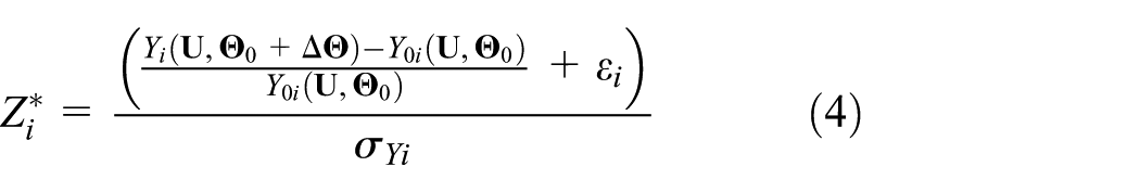
Although engine deterioration affects measured and monitored gas path variables, the impact of the changes in operating and environmental conditions is by far more significant. For this reason, a gas turbine diagnostic process usually includes a preliminary stage for computing deviations, which are free of the influence of these conditions, revealing degradation effects.^14,15 Deviations are defined as relative differences between measured and engine baseline (healthy state) values. Since the healthy state depends on engine operating conditions, it can be written as ${\mathbf{Y}}_0(\mathbf{U})$ usually called a baseline model. In this investigation, the deviations are computed using the thermodynamic model for simulating both the baseline and the engine with faults. In this way, the relative deviations take the form

$$\delta Y_i=\frac{Y_i(\mathbf{U},{\mathbf{\Theta }}_0+\mathrm{\Delta }\mathbf{\Theta })-Y_{0i}(\mathbf{U},{\mathbf{\Theta }}_0)}{Y_{0i}(\mathbf{U},{\mathbf{\Theta }}_0)}i=1,\dots ,m$$

(3)

where a vector ${\mathbf{\Theta }}_0$ corresponds to a healthy engine whereas fault parameters $\mathrm{\Delta }\mathbf{\Theta }$ consider fault influence. These model-based deviations present base points to compute deviations for any value and combination of fault parameters. The deviation computation for an arbitrary fault parameter value is performed by a piecewise-linear interpolation between the base points. The deviation corresponding to some fault parameters is determined by the sum of their individual influences. Simulated deviations can be more realistic adding a normally distributed random noise ${\epsilon }_i$ . Additionally, to have a homogeneous diagnostic space, deviations are normalized resulting in the following

$$Z_i^{*}=\frac{(\frac{Y_i(\mathbf{U},{\mathbf{\Theta }}_0+\mathrm{\Delta }\mathbf{\Theta })-Y_{0i}(\mathbf{U},{\mathbf{\Theta }}_0)}{Y_{0i}(\mathbf{U},{\mathbf{\Theta }}_0)}+{\epsilon }_i)}{{\sigma }_{\mathrm{Yi}}}$$

(4)

where ${\sigma }_{\mathrm{Yi}}$ is the amplitude of possible random fluctuations in the original deviation $\delta Y_i$ . Normalized deviations of all monitored variables constitute an $(m\times 1)$ -vector ${\mathbf{Z}}^{*}$ forming a diagnostic space where the fault classification is constructed. A pattern to be recognized represents a vector in this space.

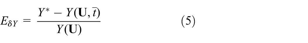
Although the use of simulated deviation measurement noise in gas turbine diagnostic algorithms is a common practice, real deviation errors can present different distributions that can affect the final diagnosis reliability. A procedure proposed to extract error components from deviations working with real data can be found in Loboda et al. ⁵ A degraded engine model $\mathbf{Y}(\mathbf{U},\overline{t})$ obtained by the least-squares method and input data including multiple operating points with different degradation severity are required. Using this model, a real deviation error can be given as follows

$$E_{\delta Y}=\frac{Y^{*}-Y(\mathbf{U},\overline{t})}{Y(\mathbf{U})}$$

(5)

Fault classification construction

After generating the model-based normalized deviations, they are used to build fault classifications required for diagnostics. Given that faults vary significantly in practice, it is necessary to describe them using a limited number of classes. ¹⁶ Each fault class is constructed from patterns, either with the change in one fault parameter (single-fault class) or with the independent change in some fault parameters (multiple-fault class). This last type of class can be explained by the fact that faults can simultaneously appear in different engine components.

A uniform distribution of fault parameter values inside of interval (0, ±5%) is employed to describe random fault severity. The limit “0” gives the possibility to simulate no-fault states while the limit “±5%” corresponds to the maximal change in the component performances, at which gas turbines lose their operation capacity due to deterioration and faults.^11,17 To know whether a current pattern ${\mathbf{Z}}^{*}$ belongs to a specific class $D_j$ , the criterion $R_j=R({\mathbf{Z}}^{*},D_j)$ , $j=1,\dots ,q$ is applied. When all values $R_j$ are obtained, a decision rule can be applied as follows

$$d=d_l\mathrm{if}{R}_l=max(R_1,R_2,\dots ,R_q)$$

(6)

where $d$ is a possible diagnosis corresponding to a correct classification. This subsection only introduces the general idea of fault classification construction. The principle of a variable structure classification and a new fault severity boundary are explained in detail in section “Fault classification.”

Training and validation

A learning set ${\mathbf{Z}}_L$ includes patterns of all classes and is employed to train the techniques under analysis. Every technique is trained on known entry pairs: the input pattern vector ${\mathbf{Z}}^{*}$ and its target. Since it is not sufficient to achieve high accuracy in training, a common strategy is to have additional data for validation and pay attention to its accuracy. ⁸ In this way, the proposed validation set ${\mathbf{Z}}_V$ verifies whether the technique can generalize the fault description. This set is created in the same way as ${\mathbf{Z}}_L$ . The only exception is the use of different series of random numbers that are involved in the computation of fault severity and errors in the deviations. As in the case of the learning set, every pattern in the validation set belongs to a known class.

Evaluation criterion (diagnosis accuracy)

In an effort to tune and compare all the techniques proposed, an averaged accuracy performance is determined for each of them. The technique analyzed classifies the patterns of the set ${\mathbf{Z}}_V$ , producing the diagnosis $d_j$ . Comparing $d_j$ with a known class $D_l$ for all validation set patterns, a confusion matrix is formed (Table 9 in Appendix 1), whose diagonal contains a vector $\mathbf{P}$ of correct pattern classification probabilities (a.k.a. true positive rates) for each fault class.^11,18 A mean number $\overline{P}$ of these probabilities determines the total accuracy of engine fault recognition. It is a criterion to tune and evaluate the techniques. By analyzing the confusion matrix itself, the direct influence of certain fault classes on the final diagnosis is visible.

Tuning

In order to perform an adequate evaluation, internal parameters of each technique should be tailored to ensure the maximal probability $\overline{P}$ . ¹⁹ For MLP, the principal parameters to tune are the number of iterations, the type of backpropagation training algorithm, and the number of hidden layer neurons. In the case of RBN, the spread $\sigma$ and the number of hidden layer neurons are varied independently until the best combination producing the highest $\overline{P}$ is selected. As for PNN, the only parameter to tailor is the spread $\sigma$ . Finally, SVMs use k-fold cross validation to improve the prediction accuracy. Since this work uses the RBF kernel, ¹⁸ the parameters to tune are $\sigma$ and the regularization parameter $C$ . It is not known with anticipation which $C$ and $\sigma$ are the most appropriate to accurately predict unknown data. In order to find these parameters, a grid search with exponentially growing sequences of $C$ and $\sigma$ is applied. It allows finding the combination of parameters that yields the lowest generalization error giving the highest diagnosis accuracy.

Fault classification

Fault classification variations

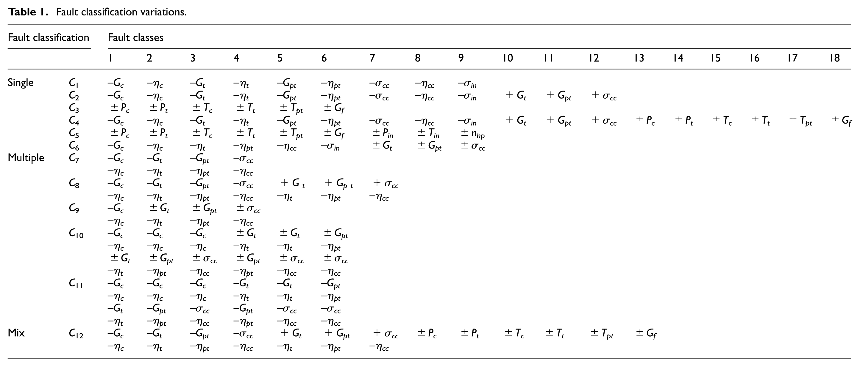
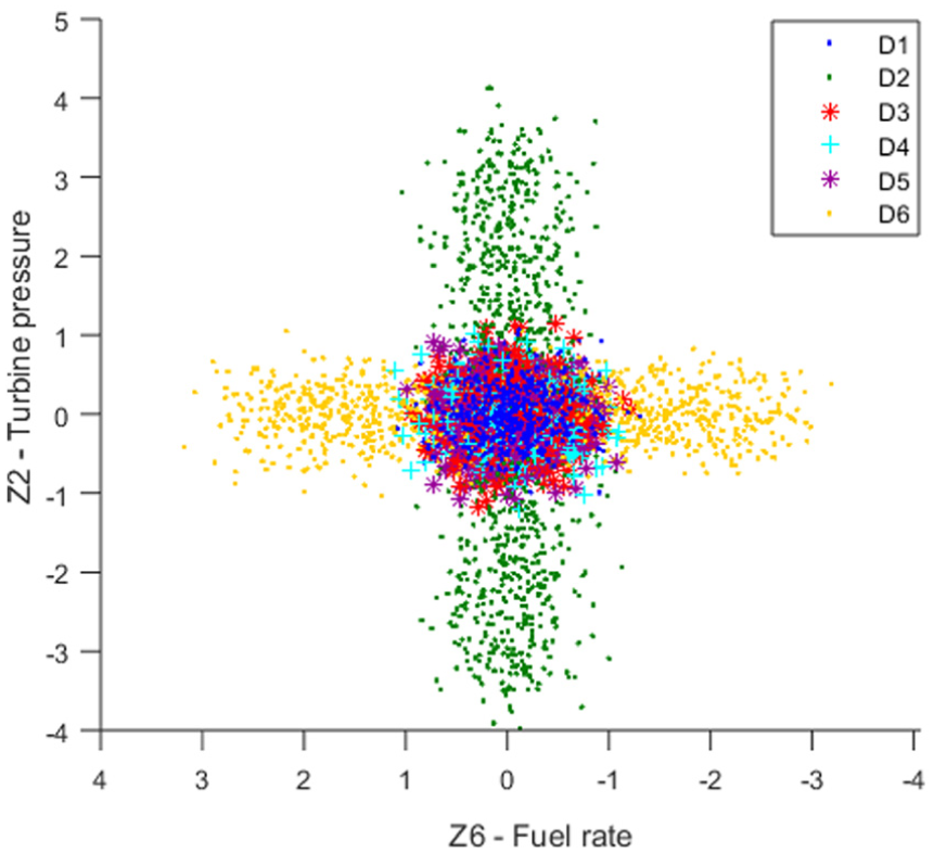
Based on the idea that gas turbine fault classifications vary widely in practice, this article proposes a principle of variable classification through an algorithm that allows changing in a flexible and easy way the following elements: type of class used (single, multiple, or mixed classes), pattern numbers, fault severity, class quantity, fault development directions (positive or negative changes), operating mode, noise scheme in deviations, type of boundary, and engine components. Thus, the algorithm developed can work with more realistic fault classes. With the intention of studying the influence of classification structure on the final diagnostic accuracy of each technique, 12 fault classifications are introduced using this algorithm. These classifications are specified in Table 1 and briefly described below. The fault parameter symbol description can be found in Table 7 in Appendix 1. Figures 3–6 present some classifications plotted in the diagnostic space of $\mathbf{Z}$ , illustrating great differences in classification-to-classification pattern distributions. Thus, the recognition techniques will be evaluated under multiple and very different conditions.

Table 1.

Fault classification variations.

Fault classification		Fault classes
		1	2	3	4	5	6	7	8	9	10	11	12	13	14	15	16	17	18
Single	C 1	−Gc	−ηc	−Gt	−ηt	−Gpt	−ηpt	−σcc	−ηcc	−σin
	C 2	−Gc	−ηc	−Gt	−ηt	−Gpt	−ηpt	−σcc	−ηcc	−σin	+Gt	+Gpt	+σcc
	C 3	±Pc	±Pt	±Tc	±Tt	±Tpt	±Gf
	C 4	−Gc	−ηc	−Gt	−ηt	−Gpt	−ηpt	−σcc	−ηcc	−σin	+Gt	+Gpt	+σcc	±Pc	±Pt	±Tc	±Tt	±Tpt	±Gf
	C 5	±Pc	±Pt	±Tc	±Tt	±Tpt	±Gf	±Pin	±Tin	±nhp
	C 6	−Gc	−ηc	−ηt	−ηpt	−ηcc	−σin	±Gt	±Gpt	±σcc
Multiple	C 7	−Gc	−Gt	−Gpt	−σcc
		−ηc	−ηt	−ηpt	−ηcc
	C 8	−Gc	−Gt	−Gpt	−σcc	+G t	+Gp t	+σcc
		−ηc	−ηt	−ηpt	−ηcc	−ηt	−ηpt	−ηcc
	C 9	−Gc	±Gt	±Gpt	±σcc
		−ηc	−ηt	−ηpt	−ηcc
	C 10	−Gc	−Gc	−Gc	±Gt	±Gt	±Gpt
		−ηc	−ηc	−ηc	−ηt	−ηt	−ηpt
		±Gt	±Gpt	±σcc	±Gpt	±σcc	±σcc
		−ηt	−ηpt	−ηcc	−ηpt	−ηcc	−ηcc
	C 11	−Gc	−Gc	−Gc	−Gt	−Gt	−Gpt
		−ηc	−ηc	−ηc	−ηt	−ηt	−ηpt
		−Gt	−Gpt	−σcc	−Gpt	−σcc	−σcc
		−ηt	−ηpt	−ηcc	−ηpt	−ηcc	−ηcc
Mix	C 12	−Gc	−Gt	−Gpt	−σcc	+Gt	+Gpt	+σcc	±Pc	±Pt	±Tc	±Tt	±Tpt	±Gf
		−ηc	−ηt	−ηpt	−ηcc	−ηt	−ηpt	−ηcc

Figure 3.

Fault classification 3.

Figure 4.

Fault classification 7.

Figure 5.

Fault classification 10.

Figure 6.

Fault classification 11.

Single-fault classifications

As shown in Table 1, Classification 1 consists of nine single faults. Each fault is created by varying one gas path fault parameter in the negative direction. Classification 2 considers erosion and burnouts of hot part elements that can cause the increase in their flow performances. For this reason, positive changes for flow parameters of the CT, PT, and CC are introduced. With these parameters, three new classes are formed and added to Classification 1 resulting in 12 classes. Due to the frequency of sensor malfunctions, they are recommended to be diagnosed along with gas path faults. Since great measurement biases are easy to identify, only hidden incipient sensor faults are considered (small bias interval of ±5%). In this way, for six monitored variables, six corresponding single classes form Classification 3. Figure 3 shows these six gas path sensor faults; however, only those coinciding with their monitored variables can be completely observed (green and yellow classes). Classification 4 joins Classifications 2 and 3 to build 18 single classes representing gas path faults and sensor malfunctions. Also, sensor malfunctions of operating condition parameters are simulated to take into account their influence on all monitored variables. Three single classes of this sensor fault type are created and joined to the previous six sensor faults (monitored variables) forming nine classes for Classification 5. Classification 6 considers nine classes: one compressor air flow fault, four efficiency faults for all components, one inlet pressure loses factor fault, and finally, three faults with double direction for CT, PT, and CC.

Multiple-fault classifications

Classification 7 includes four multiple classes grouped by engine component: C, CC, CT, and PT (Figure 4). These classes are formed by independent variation in two fault parameters of the same component. Classification 8 contains seven classes formed by three multiple classes with positive changes for flow parameters and their respective efficiencies (Classification 2) and four classes from Classification 7. For Classification 9, four classes are formed as Classification 7 with the difference that flow parameters change in two directions for CT, PT, and CC. Classification 10 contains six classes, each one created by four fault parameters (some of them with two fault development directions). It is formed by all possible combinations of C, CC, CT, and PT (Figure 5). Classification 10 is closer to what really happens in a real gas turbine engine because it considers faults that can occur in two components at the same time. As for Classification 11, it is built in the same manner as the previous classification with the difference that the six classes include negative fault parameter changes (Figure 6).

Single- and multiple-fault classification

Classification 12 works with 13 classes formed with 7 multiple classes from Classification 8 and 6 single classes from Classification 3. The next subsection presents different boundaries used for multiple-fault classifications.

Multiple-class boundaries

When multiple faults are simulated by summing the influence of each fault parameter, there is a risk that the simulated fault exceeds the severity limit of real faults. To better understand the problem, let us consider a multiple class $D_1$ created by two fault parameters represented by vectors 0–L₁ and 0–L₂ in Figure 7. The point “0” corresponds here to an engine normal state. Each of the vectors 0–L₁ and 0–L₂ reflects theoretical changes in one fault parameter. Fault severity increases to the engine health limit formed by points $L_1$ and $L_2$ and vector lengths $l_1$ and $l_2$ . It is clear that vector $\mathbf{Z}$ (without errors ${\epsilon }_i$ ) in the dotted part of the parallelogram can be longer than base vectors 0–L₁ and 0–L₂ produced by a maximal change in the corresponding fault parameters. In other words, simulated faults can have higher severity than real ones. In order to avoid this and to make a class formation more realistic, a linear boundary L₁L₂ that restricts fault pattern vectors inside the triangle 0–L₁L₂ was previously used. ⁴ However, that boundary is too restrictive when the angle ${\theta }_{12}$ increases.

Figure 7.

Three boundaries for multiple classes.

It seems to us that a more appropriate boundary would be a smooth curve. For this reason, a new multiple-class boundary based on the Archimedean spiral is proposed (Figure 7). It is formed by the vector (blue line) that moves from $L_1$ to $L_2$ and gradually changes its length $l$ from $l_1$ to $l_2$ proportionally to the turning angle. Thus, this length can be expressed as follows

$$l=l_1+(l_2-l_1)\frac{{\theta }_i}{{\theta }_{12}}$$

(7)

where ${\theta }_i$ is the angle between the current vector and the first base vector for a random pattern $i$ , and ${\theta }_{12}$ is the angle between the two base vectors. Only the deviation vector $\mathbf{Z}$ that is inside the curve is accepted. The described boundary can be easily extended to three fault parameters. The boundary vector of the length $l$ determined in the plane of the first and second fault parameters (blue line) now is considered as a base vector. The second base vector 0–L₃ is produced by a third fault parameter. The boundary is determined in the plane of these two base vectors and is created in the same way, with a vector (orange line) that gradually changes its length from $l_3$ to $l$ . For the case of four and more fault parameters, the boundary is determined similarly. A restrictive condition of this boundary is great for small angles between base vectors and decreases along with the increase in angle.

In order to determine the effect of the new boundary, this article analyzes the three boundaries described before. They are named as “straight line” for the triangle area, “no boundary” for the parallelogram area, and “Archimedean” for the new boundary. For all these boundaries, the corresponding classifications are constructed and the four mentioned techniques are applied.

Technique evaluation results

The probability of correct diagnosis (diagnosis accuracy indicator) is used as a criterion to evaluate the performance of each technique in gas turbine fault recognition. Four comparative studies are considered. They are formed by varying

1. Different pattern numbers

2. Different operating modes

3. Different fault boundaries

4. Different deviation noise schemes

Within each study, in addition to the varying factor, the fault classification changes as well. The variation in the conditions allows drawing solid conclusions about the best technique. The studies are shortly described below.

Different pattern numbers

Accuracy of fault classes’ description depends on the number of simulated patterns; nevertheless, sometimes it is not possible to obtain sufficient data to achieve it. ²⁰ In order to address this hypothetical lack of information and analyze its effect on the diagnosis accuracy for each technique, 10 pattern numbers are analyzed ranging from 100 to 1000 using four classification variations. Initially, calculations are based on 1 seed, which is a parameter for initiating a random number series (one calculation of $\overline{P}$ ). However, during experimentation, different seeds yield different probabilities of correct diagnosis. To reduce the error produced by this randomness, calculations with 100 seeds are performed and averaged. Figure 8 and Table 2 show the results obtained for 100 seeds working with four classifications. The first impression is that RBN is the best technique in Classification 3, SVM in Classification 4, MLP and RBN in Classification 9, and MLP and SVM in Classification 10. Since this is not sufficient to select the best technique, total average probabilities considering all pattern numbers and all classification variations are obtained to know the overall fault recognition performance of each technique. The probabilities are 0.7922 for MLP, 0.8039 for RBN, 0.8001 for PNN, and 0.8122 for SVM. As can be seen, the ANN techniques have very similar diagnosis probabilities (a difference of 1.17% between them); however, SVM is slightly better than all of them (2% over MLP, 0.83% over RBN, and 1.21% over PNN).

Figure 8.

Diagnosis accuracy comparison between ANNs and SVMs for different pattern numbers (100 seeds).

Table 2.

Diagnosis accuracy $\overline{P}$ for different pattern numbers (100 seeds).

Fault classification	Method	Number of patterns										Average	Total average
		100	200	300	400	500	600	700	800	900	1000
C 3	MLP	0.7382	0.7576	0.7763	0.7750	0.7807	0.7875	0.7887	0.7975	0.8015	0.7960	0.7799	All pattern numbers and all classificationsMLP = 0.7922RBN = 0.8039PNN = 0.8001SVM = 0.8122100 patterns and all classificationsMLP = 0.7612RBN = 0.7883PNN = 0.7739SVM = 0.7893
	RBN	0.7973	0.8040	0.8068	0.8080	0.8076	0.8084	0.8083	0.8081	0.8081	0.8081	0.8065
	PNN	0.7897	0.7956	0.7991	0.7893	0.7978	0.8017	0.8024	0.8026	0.8034	0.8036	0.7985
	SVM	0.7859	0.7930	0.7903	0.7971	0.7982	0.7946	0.8018	0.7961	0.7964	0.8036	0.7957
C 4	MLP	0.6446	0.6569	0.6630	0.6677	0.6692	0.6738	0.6850	0.6871	0.6848	0.6906	0.6722
	RBN	0.7049	0.6982	0.6888	0.7173	0.6954	0.7160	0.7161	0.7191	0.7179	0.7174	0.7091
	PNN	0.7154	0.7217	0.7289	0.7303	0.7316	0.7326	0.7339	0.7352	0.7350	0.7352	0.7300
	SVM	0.7250	0.7312	0.7359	0.7374	0.7381	0.7390	0.7398	0.7409	0.7403	0.7405	0.7368
C 9	MLP	0.9135	0.9164	0.9249	0.9273	0.9287	0.9284	0.9284	0.9294	0.9297	0.9296	0.9256
	RBN	0.9117	0.9210	0.9240	0.9262	0.9280	0.9278	0.9290	0.9297	0.9300	0.9301	0.9258
	PNN	0.9054	0.9158	0.9150	0.9219	0.9213	0.9242	0.9251	0.9255	0.9265	0.9260	0.9207
	SVM	0.8939	0.9166	0.9225	0.9250	0.9263	0.9225	0.9279	0.9283	0.9297	0.9294	0.9222
C 10	MLP	0.7486	0.7758	0.7874	0.7941	0.7978	0.7898	0.8022	0.8027	0.8048	0.8062	0.7909
	RBN	0.7395	0.7668	0.7735	0.7772	0.7786	0.7784	0.7790	0.7850	0.7845	0.7812	0.7744
	PNN	0.6852	0.7217	0.7398	0.7513	0.7569	0.7637	0.7688	0.7717	0.7753	0.7775	0.7512
	SVM	0.7526	0.7772	0.7904	0.7887	0.8002	0.8020	0.8049	0.8071	0.8084	0.8091	0.7941

MLP: multi-layer perceptron; RBN: radial basis network; PNN: probabilistic neural network; SVM: support vector machine.

Also, total average probabilities for only 100 patterns and all classifications are obtained for all the techniques. The results are as follows: 0.7612 for MLP, 0.7883 for RBN, 0.7739 for PNN, and 0.7893 for SVM. Again, SVM obtained slightly better probabilities (2.81% over MLP, 0.1% over RBN, and 1.54% over PNN). However, it is visible that the difference between SVMs and RBN is negligible. This is important because SVMs are generally claimed to have better generalization than ANNs when working with small samples. As a final remark, the increase in the pattern number influenced positively the resolution capability for all techniques (up to 9%). However, a drawback is that more execution time and computer memory are required. This is very notorious in parameter tuning stage because a lot of computations are performed before selecting the most appropriate model giving us the highest probability $\overline{P}$ . For that reason, the pattern number is a compromise between diagnosis accuracy and computer requirements.

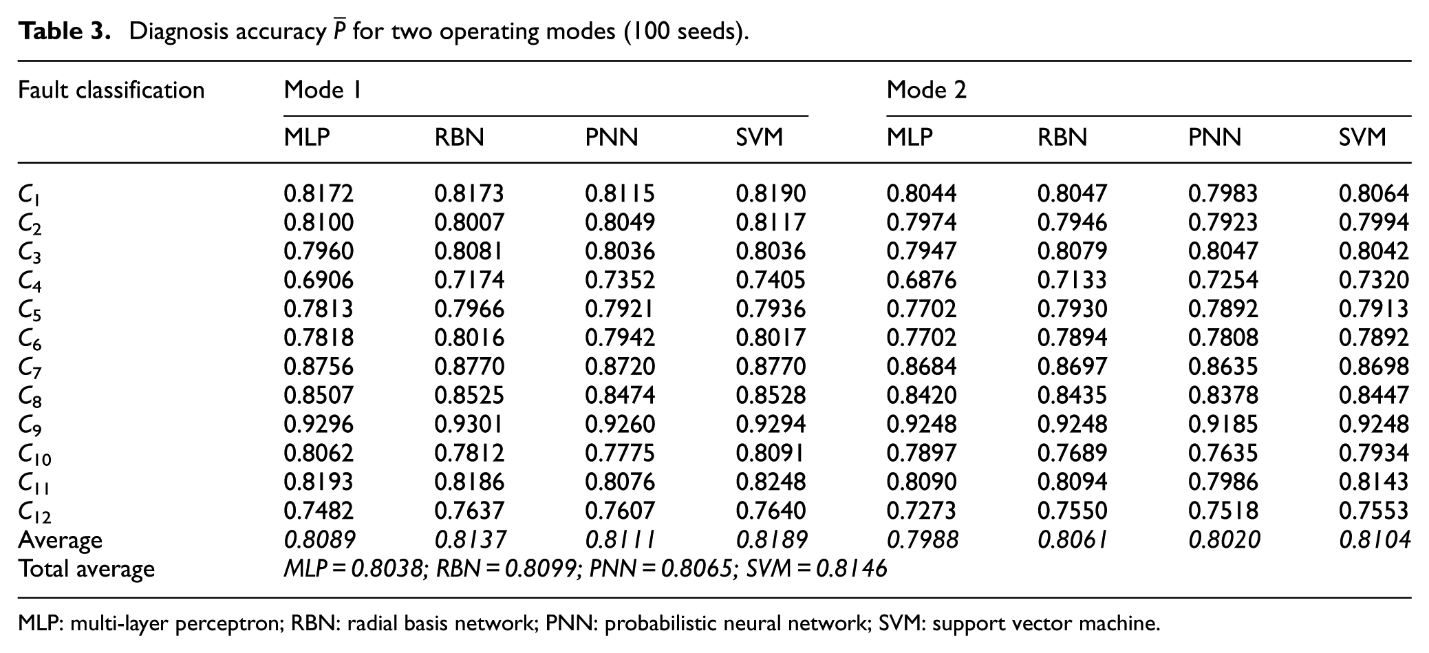
Different operating modes

Two gas turbine operating modes, Mode 1 and Mode 2, are studied. They are close to engine maximal and idle regimes and are set by different high-pressure rotor speeds under standard atmospheric conditions. The analysis considers all the classification variations. Based on the above results for pattern numbers, this comparative study only works with 1000 patterns to have more accurate results. The results obtained are presented in Figures 9 and 10 and Table 3. Considering both modes, SVM is slightly better with a total average probability of 0.8146. RBN is the second best technique (being the winner in some classifications) with 0.8099. PNN is in the third position with 0.8065 and MLP is the last technique with 0.8038 of performance. Nevertheless, the difference between all the techniques is not so great (1.08%). Another important observation is that for Mode 2, the probabilities are lower than Mode 1 for most of the classifications. However, the averaged difference between both modes is small (about 0.0088). Besides, the probability behavior of the techniques is almost the same for the two modes through all classifications. Taking into account that the random errors in the stochastic simulation remain small due to the 100 seeds calculation, the results presented can be more reliable. Thus, we can conclude that the change in operating mode of the analyzed gas turbine does not affect the performance of techniques.

Figure 9.

Diagnosis accuracy comparison between ANNs and SVMs for operating mode 1 (100 seeds).

Figure 10.

Diagnosis accuracy comparison between ANNs and SVMs for operating mode 2 (100 seeds).

Table 3.

Diagnosis accuracy $\overline{P}$ for two operating modes (100 seeds).

Fault classification	Mode 1				Mode 2
	MLP	RBN	PNN	SVM	MLP	RBN	PNN	SVM
C 1	0.8172	0.8173	0.8115	0.8190	0.8044	0.8047	0.7983	0.8064
C 2	0.8100	0.8007	0.8049	0.8117	0.7974	0.7946	0.7923	0.7994
C 3	0.7960	0.8081	0.8036	0.8036	0.7947	0.8079	0.8047	0.8042
C 4	0.6906	0.7174	0.7352	0.7405	0.6876	0.7133	0.7254	0.7320
C 5	0.7813	0.7966	0.7921	0.7936	0.7702	0.7930	0.7892	0.7913
C 6	0.7818	0.8016	0.7942	0.8017	0.7702	0.7894	0.7808	0.7892
C 7	0.8756	0.8770	0.8720	0.8770	0.8684	0.8697	0.8635	0.8698
C 8	0.8507	0.8525	0.8474	0.8528	0.8420	0.8435	0.8378	0.8447
C 9	0.9296	0.9301	0.9260	0.9294	0.9248	0.9248	0.9185	0.9248
C 10	0.8062	0.7812	0.7775	0.8091	0.7897	0.7689	0.7635	0.7934
C 11	0.8193	0.8186	0.8076	0.8248	0.8090	0.8094	0.7986	0.8143
C 12	0.7482	0.7637	0.7607	0.7640	0.7273	0.7550	0.7518	0.7553
Average	0.8089	0.8137	0.8111	0.8189	0.7988	0.8061	0.8020	0.8104
Total average	MLP = 0.8038; RBN = 0.8099; PNN = 0.8065; SVM = 0.8146

MLP: multi-layer perceptron; RBN: radial basis network; PNN: probabilistic neural network; SVM: support vector machine.

Different fault boundaries

Three boundary options are examined: no boundary (parallelogram area), straight line (triangle area), and Archimedean spiral. They are applied to multiple faults of classification variations 7 and 11. For each boundary and variation, the four techniques are used by turn for computing diagnosis probabilities $\overline{P}$ considering 100 seeds. Figures 11 and 12 and Table 4 contain all the results that help draw the following conclusions. First, the total average probability for each technique is 0.8229 for MLP, 0.8222 for RBN, 0.8146 for PNN, and 0.8248 for SVM. It is evident that the highest value is produced by SVM and the lowest one by PNN. However, the difference between the four recognition techniques remains small (1.02%). Second, the new boundary results in a visible change in the probability $\overline{P}$ . This change can be greater (up to 25%) for particular cases, for example, the “Straight line” boundary in Classification 11 where probabilities are very low. Third, for all cases, the “Archimedean spiral” probability occupies an intermediate position between “No boundary” probability and “Straight line” probability. This is easily explained by the fact that the Archimedean spiral curve is situated between the straight line and the parallelogram sides.

Figure 11.

Diagnosis accuracy for different boundaries (classification 7).

Figure 12.

Diagnosis accuracy for different boundaries (classification 11).

Table 4.

Diagnosis accuracy $\overline{P}$ for different boundaries (100 seeds).

Fault classification	Multiple-class boundary	MLP	RBN	PNN	SVM
C 7	Straight line	0.8756	0.8770	0.8720	0.8770
	No boundary	0.9174	0.9181	0.9140	0.9182
	Archimedean	0.9126	0.9130	0.9078	0.9110
C 11	Straight line	0.5834	0.5839	0.5703	0.5875
	No boundary	0.8289	0.8223	0.8156	0.8301
	Archimedean	0.8193	0.8186	0.8076	0.8248
	Total average	0.8229	0.8222	0.8146	0.8248

MLP: multi-layer perceptron; RBN: radial basis network; PNN: probabilistic neural network; SVM: support vector machine.

Different deviation noise schemes

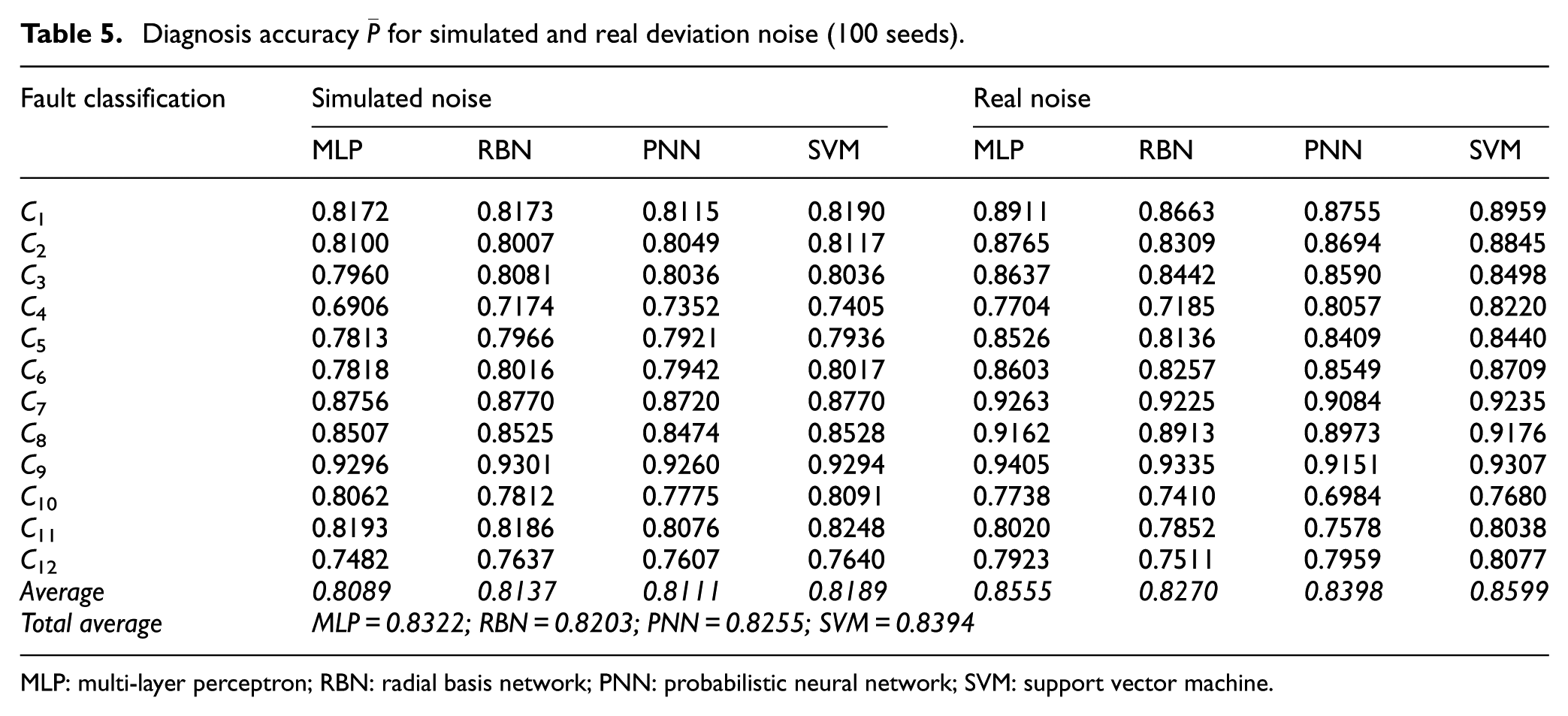
Two schemes of deviation noise are studied: simulated and real noise. The real noise was extracted from deviations using real data recorded hourly at steady-state operating points of the same gas turbine engine presented in subsection “Test case engine.” The following elements are considered for the comparison: all the fault classifications, maximal operating mode, and 1000 patterns. Table 5 shows the results for both error schemes. Figure 13 presents the results for real deviation errors. The results for the simulated scheme are the same as Figure 9 shown before. Comparing both error representations, one can see a significant increase in diagnosis accuracy for all the techniques (4.66% for MLP, 1.33% for RBN, 2.87% for PNN, and 4.10% for SVM). The total average probability of each technique is obtained as before by averaging both error schemes. The results are 0.8322 for MLP, 0.8203 for RBN, 0.8255 for PNN, and 0.8394 for SVM. Again, the highest value is produced by SVM. However, this time, RBN is the lowest one and MLP has a much better performance than in the case of simulated noise. As mentioned before, the difference between techniques is not so great for simulated errors (about 1.07%), while for real errors is a little bit greater (about 3.29%). This can be proven by analyzing classification-to-classification probabilities. In classification 2, 4, 6 and 12 there are evident differences between the highest value (SVM) and the lowest one (RBN). This means that the use of more realistic deviation noise representation does affect the performance of techniques. In contrast to simulated errors, where RBN is the second best technique, the use of real noise negatively affects the technique being the one with the lowest probability for that case. Besides, it requires more training time than usual.

Table 5.

Diagnosis accuracy $\overline{P}$ for simulated and real deviation noise (100 seeds).

Fault classification	Simulated noise				Real noise
	MLP	RBN	PNN	SVM	MLP	RBN	PNN	SVM
C 1	0.8172	0.8173	0.8115	0.8190	0.8911	0.8663	0.8755	0.8959
C 2	0.8100	0.8007	0.8049	0.8117	0.8765	0.8309	0.8694	0.8845
C 3	0.7960	0.8081	0.8036	0.8036	0.8637	0.8442	0.8590	0.8498
C 4	0.6906	0.7174	0.7352	0.7405	0.7704	0.7185	0.8057	0.8220
C 5	0.7813	0.7966	0.7921	0.7936	0.8526	0.8136	0.8409	0.8440
C 6	0.7818	0.8016	0.7942	0.8017	0.8603	0.8257	0.8549	0.8709
C 7	0.8756	0.8770	0.8720	0.8770	0.9263	0.9225	0.9084	0.9235
C 8	0.8507	0.8525	0.8474	0.8528	0.9162	0.8913	0.8973	0.9176
C 9	0.9296	0.9301	0.9260	0.9294	0.9405	0.9335	0.9151	0.9307
C 10	0.8062	0.7812	0.7775	0.8091	0.7738	0.7410	0.6984	0.7680
C 11	0.8193	0.8186	0.8076	0.8248	0.8020	0.7852	0.7578	0.8038
C 12	0.7482	0.7637	0.7607	0.7640	0.7923	0.7511	0.7959	0.8077
Average	0.8089	0.8137	0.8111	0.8189	0.8555	0.8270	0.8398	0.8599
Total average	MLP = 0.8322; RBN = 0.8203; PNN = 0.8255; SVM = 0.8394

MLP: multi-layer perceptron; RBN: radial basis network; PNN: probabilistic neural network; SVM: support vector machine.

Figure 13.

Diagnosis accuracy comparison between ANNs and SVMs for real deviation errors (100 seeds).

Discussion

The following explanations summarize the main contributions of this article:

1. For variable gas turbine fault conditions, any technique presented in this investigation can be an efficient option. Although SVMs produced better results for all the comparative studies analyzed, the difference between all the techniques in terms of $\overline{P}$ is not so great. Furthermore, the similar probabilities prove that the methods are near the theoretical accuracy levels intrinsically related to the engine and the type of fault classification studied and the four techniques are advanced enough to correctly perform the recognition task. Thus, no other technique will significantly increase the probability of correct classification. Since the evaluation criterion $\overline{P}$ may not be sufficient to select an appropriate technique, there are other important aspects to take into consideration. In the case of MLP, the existence of local minima complicated considerably the training stage. Besides, it has more parameters to tune, for example, the number of hidden neurons, the number of iterations, the training goal, and the parameters of the backpropagation method selected. The advantage of MLP is its easiness to implement. As for RBN, it only needs two parameters to be tuned; however, many calculations must be done. Furthermore, it requires much more computational resources and time for training making this technique the least recommended for real training stages. PNN is the simplest gas turbine fault recognition technique and only needs one parameter to tune (σ) resulting in a faster training stage. Also, it has the important advantage of providing confidence estimations for every diagnostic decision which make it a very good option for real monitoring systems. One disadvantage of PNN is the need of more computational resources to store the model when the number of patterns is increased. SVM is the technique that achieves slightly better results and only needs two parameters to be tuned (σ and C). Also, it is not limited by the computational memory supporting more number of patterns. However, one disadvantage of SVM is that its training can be very slow compared to the rest of techniques when the data are increased.

2. Based on the principle of variable classification, the results obtained for all the comparative studies confirm that there is a great influence of the fault classifications on the diagnosis accuracy levels. Thus, this article gives an idea on how the theoretical accuracy levels behave for different gas turbine fault identification conditions, serving as a help in the decisions of real engine monitoring designers. The principle allows us to create different classifications with necessary totality of fault classes of different type and complexity. The formation of each new classification and change from one classification to another one is simple and do not need to reprogram the algorithm. In general, the diagnosis probabilities generated for all the classifications are acceptable taking into account that the classes are more complex. This complexity can be seen, for example, in classification 4, where there are up to 18 classes and most of them intersect in the center. Also, the increasing number of fault parameters to form multiple classes and other characteristics such as the number of patterns per class, the fault development directions, and the type of fault class complicate the recognition task for all the techniques.

3. There is an important effect of fault severity boundary on the probabilities of correct diagnosis. With these results, the new boundary makes the simulation more realistic and allows determining more precisely the level of diagnostic accuracy. The fault severity limits of the multiple classes are smoother, which could be the behavior in real faulty conditions. For this reason, the new boundary is advisable for future works.

4. The use of real deviation noise in fault class description provides more accurate simulation of a diagnostic process and provides more reliable level of diagnostic accuracy. This real noise scheme significantly changed the final diagnosis accuracy in all the fault classifications and all the techniques as well.

Some proposed works in the near future may involve recent and fast ANNs learning algorithms,^21,22 approaches based on deep learning, measurement inaccuracy and deviation error reduction analysis, non-measured gas turbine variables such as thrust and efficiency as alternative parameters for engine condition monitoring, novel signal processing approaches for gas turbine diagnostics, different distributions employed to describe random fault severity, and mixed data-driven and model-based fault classification to have an even more realistic fault recognition problem.

Conclusion

The intention of this study was to evaluate four fault recognition techniques (three ANNs and one SVMs) and analyze how they behave under more versatile, realistic, and complex fault conditions. The ANNs analyzed were MLP, RBN, and PNN. A principle of a variable fault classification was proposed to enhance the representation of real fault scenarios. In all, 12 complex classifications were created considering this principle and used to compare the methods. Also, a new boundary for fault severity was introduced in the fault class description. The techniques were analyzed using a comparison procedure that computed for each of them a probability of correct diagnosis, which was the principal criterion for evaluation. In order to draw concise conclusions, four comparative studies were considered.

The results obtained for multiple comparison cases have shown that nearly always the techniques under analysis are very close using the criterion of correct diagnosis probability. A total level of diagnostic accuracy changed from case to case much more than the differences between the techniques applied to the same comparison case. On average, for all multiple and very different studies, it is concluded that any of the four techniques is a good alternative for gas turbine fault identification. However, in addition to the average accuracy, the SVMs and ANNs have other advantages and disadvantages related to computational requirements and execution time that should be taken into consideration if these techniques are implemented in real monitoring systems. Extensive comparison calculations have also revealed a great influence of fault classifications and fault severity boundary on the level of diagnostic accuracy. The implementation of the new boundary and real errors in deviations makes the engine diagnostic accuracy closer to what occurs in practice.