Sage Journals: Discover world-class research

Abstract

As one of the major causes of traffic accidents, tire hydroplaning is a key driver safety concern. A tire model 205/55R16 was employed in this study, and a virtual simulation of a deformed half-tire domain for calculating hydroplaning speed was built by virtue of computational fluid dynamics. Water-flow field characteristics were simulated using gas–liquid two-phase flow. The simulated tire hydroplaning speed is in accord with the measured tire hydroplaning data. Guided by the idea that the drag-reduction effect of the V-riblets based on bionic study of shark skin, effects of V-riblet bionic non-smooth surface parameters on water displacement, and flow resistance were analyzed to improve tire tread pattern draining capacity. The water drag-reduction mechanism was declared by the vortex vector and speed field, and the optimal V-riblet surface for drag reduction was set on the bottom circumferential grooves to analyze hydroplaning speed. The results demonstrate that the V-riblet bionic non-smooth surface can effectively decrease tread hydrodynamic pressure when driving on a water-film and increase tire hydroplaning speed.

Keywords

Tire hydroplaning V-riblet surface numerical simulation computational fluid dynamics

Introduction

Various traffic safety studies all over the world indicate that about 20% of road accidents occur in wet weather conditions. Although there are no detailed statistics concerning the exact nature of these wet weather hazardous, it is generally believed that tire hydroplaning is one of the major contributing factors. When a tire hydroplanes on wet pavements, the driver loses both steering and braking control. Comprehensive understanding of this phenomenon will help reduce high-risk traffic accidents. Several factors contribute to hydroplaning, including water-film depth, pavement texture properties, and tire characteristics. Many previous studies have been conducted to experimentally investigate the influence of tire characteristics, inflation pressure, driving conditions, and water-film thickness on tire hydroplaning performance.¹ These studies have shed light on different factors affecting hydroplaning and resulted in useful reduction measures, including increased tread pattern width and depth and enlarged pavement grooving. Experimentation on this scale requires a test set-up and strict test specification. In addition, both of which are time consuming. To investigate the hydroplaning performance of a tire, analytical theory, hydroplaning lubrication, viscous lubrication, and boundary layer lubrication have been employed by researchers in previous studies. Unfortunately, due to the non-linearity of fluid flow, there is no strict mathematical model to predict tire deformation, and it is difficult to formulate a description of tire hydroplaning speed. Therefore, many researchers have explored the use of numerical methodology to investigate tire hydroplaning.

Researchers,² for example, built a three-dimensional simulation model of the interaction between tire and water flow using computational fluid dynamics (CFD) method. Tire surface deformation was ignored in their model; however, the computational domain remained fixed in time. The influence of hydrodynamic pressure on smooth and grooved tires with deformation was considered and the results were compared with that of the un-deformed tires. The results showed that tire deformation has a big effect on hydrodynamic pressure at higher tire speed.³ Seta et al.⁴ adopted the finite difference method (FDM) and finite element method (FEM) to simulate hydroplaning on thick water-films, under different parameters such as water-flow, speed dependence, and tread pattern effects. They found that a sloped block tip can effectively improve tire hydroplaning performance.

Cho et al.⁵ compared hydroplaning speed between different patterned tires, and they found that hydroplaning performance largely depends on the structure parameters of the tread pattern. Fwa et al.⁶ established a numerical simulation model using CFD techniques implemented in Fluent to study the effects of vertical and horizontal circumferential groove dimension on hydroplaning. They found that larger groove width and depth and smaller groove spacing can help improve hydroplaning performance. Normally, increasing the number of grooves can improve tread land–ocean comparison and provide large grooves void to drainage surface water and strengthen the force necessary to pierce the water-film. This theory of changing groove design parameters does increase hydroplaning speed; however, this method comes at the cost of crippling other tire performances. Wies et al.⁷ revealed that a 1% hydroplaning improvement by increasing the groove space will lead to 0.6% decrease in handling, 0.4% increase in rolling resistance, and 2.3% rising in rolling noise.

It is therefore necessary to find a solution to reduce water resistance and meanwhile improve the drainage capacity of tread grooves. Bio-inspired technology can provide a solution to these issues, and biomimetic drag-reduction technology facilitated tremendous achievements in the field of fluid engineering.

The NASA Research Center pointed out that shark skin has riblet groove structure distributed all over the body that reduces water resistance during high-speed swimming.⁸ Researchers have explored a number of innovative drag-reducing bio technologies. There have been remarkable achievements in bionic applications in the engineering and mechanical manufacturing fields.^9,10 For example, the frictional force using the bionic dimple structure can be reduced by as much as 7%–10% in laboratory experiments. A bionic V-riblet structure has been shown to reduce 1%–2% drag force in airplane flight tests.^11,12

Guided by the idea that the drag-reduction effect of the V-riblet is based on the bionic study of shark skin,¹³ this article proposes a procedure to design a V-riblet bionic non-smooth surface arrayed on tread circumferential grooves to remove water-flow resistance in the footprint of tread by increasing the flow rate and improve tire hydroplaning performance. First, the FEM model of a tire (205/55R16) was built with Abaqus, and by comparing tread groove deformation between test and simulation, the tire model was validated; second, the hydroplaning model was established using CFD in Fluent software, and the hydroplaning speed was analyzed. The hydroplaning speed was then compared with test data from Okano and Koishi¹⁴ to validate the hydroplaning analysis method. Third, the height and number of the V-riblet non-smooth surface with a 60° angle were set as the design parameters and the results were compared against the smooth surface grooves to obtain the priority V-riblet structure. Finally, set the optimal V-riblet structure for drag reduction on the bottom of the circumferential grooves and make the comparison of hydroplaning speed between the non-smooth surface tread grooves and smooth surface tread grooves. The results show that the V-riblet bionic non-smooth surface tread grooves can increase drainage water velocity and improve tire hydroplaning performance.

Tire FEM model and model verification

One of the main performances of tire tread groove is anti-hydroplaning. The deformation of tread under various loads affects the grooves’ drainage capability. The contact pressure and tread groove deformation under normal load must be first obtained to analyze water flow around tire–ground contact and inside the tread grooves. In this study, the FEM model of a radial tire (205/50R16) was established. The Yeoh model was adopted in the finite element analysis (FEA) of the rubber-like elastomers. The cord-rubber composite, belts, and tire carcass were modeled with rebar layers. Tire vertical deformation was achieved under the load of 4000 N and the inflation pressure of 200 kPa.

The tire static contact pressure is shown in Figure 1, and the tire footprint is obtained from the static loading machine, the MTM-2 tire testing machine, with a pressure-sensing pad, and the detailed test method was provided by Zhou et al.¹⁵ The design width and depth of the circumferential grooves are 8 mm and 9 mm, respectively. The longitudinal grooves under tire static load were chosen as the hydroplaning analysis object after the extraction of the deformed tread shape, which is shown in Figure 2(a). This was one-half of the tire model characterized by the tread’s symmetrical pattern. Using the Boolean operator “subtract,” remove tire model from water computer domain, and we can get the tire hydroplaning computational model, which is shown in Figure 2(b).

Figure 1.

Tire footprint under load.

Figure 2.

Tire model and hydroplaning: (a) half of tire model and (b) half of hydroplaning model.

The deformation of the tread pattern has a significant influence on groove water drainage. Therefore, it is necessary to acquire the deformation characteristics of the grooves before conducting any hydroplaning analysis. The results of the groove deflection test are presented in Figure 3. The SKR miniature auto-restart displacement sensor was used to monitor deflection at measurement accuracy of ±0.5%. The sensor was installed in a steel plate with a small hole with a diameter five times the size of the sensor probe.

Figure 3.

Sample tire and tire static loaded test machine.

The steel plate was placed in the drum testing machine to ensure whether the sensor probe was placed in the middle of the tread groove. A vertical load, moving up and down, was applied in the test. The groove deflection of the crown and shoulder were measured separately, and the deflection of different grooves under different loads was obtained. Tire sinkage with a load of 500 N was chosen as the deflection benchmark to avoid contact position effects between the sensor probe and the groove.

The test was conducted in the following procedure. First, a 15 mm × 15 mm rectangular hole was opened on the steel plate to facilitate displacement of the sensor probe second, two 200 × 200 wood flat with 30 × 30 gap were placed on the tire drum test bench as supporters; third, the steel plate was placed on the two pieces of wood, and the rectangular hole on the steel plate and the gap coincide with one another to facilitate the installation of displacement sensor data lines. The displacement sensor is fixed at one end of a 10 mm × 10 mm cylindrical steel pipe and the other end of the steel pipe is fixed to the tire drum test stand. According to tire coordinate, the displacement sensor is arranged at the symcenter of the longitudinal direction. Once the position is determined, the application of different loads to the tire is achieved by moving the support frame of the tire drum test stand. In order to achieve the crown groove and shoulder groove deformation, the steel plate and the two pieces of wood in the tire axial move at the same time. Tire sinkage with a load of 500 N was chosen as the deflection benchmark to avoid contact position effects between the sensor probe and the groove.

Figure 4 shows the variation of groove deflection with variation of vertical load. However, the deflection of the crown grooves was much larger than that of the shoulder grooves. The tire contact pressure distribution was presented in Figure 1. This should be beneficial for passenger car tires because the shoulder contact pressure is greater than the crown, and the tire will have improved handling performance. Groove deflection tends to be stable at 3500 N. The fact that the simulated results are so close to the measurements demonstrates the validity of the proposed tire simulation model.

Figure 4.

Deflection of tread grooves.

Tire hydroplaning analysis and method verification

Hydroplaning computational model

When a tire rolls over on a road surface in wet weather, the water and air will flow from the tire footprint zone. Therefore, the water-film model and air model should be considered in hydroplaning model. The tire contour after static deformation was created and the tire rolling state during the fluid calculation was ignored.

A domain size with a height of 50 mm, with a width of 350 mm, and a length in front of the tire of 300 mm and at the rear of the tire of 600 mm was used, as described in previous research.¹⁶ Figure 2 displays the tire hydroplaning domain, which was meshed using a locally thickened and composite meshes method. The hydroplaning domain was divided into five-sided unstructured tetrahedral mesh hybrid with structure mesh. The mesh inside the grooves and in front of the contact area was refined to ensure there were at least eight discrete units. The entire grid was composed of 1,358,587 cells and 1,272,427 nodes. Tire hydroplaning simulation was carried out using half-tire model.

Boundary conditions

When tire hydroplaning occurs, for an observer sitting in the car, hydroplaning is viewed as a rolling tire at a speed of U (m/s) sliding along a smooth flooded pavement, and this phenomenon is outlined in the fixed reference system. In the fixed reference system, the tire hydroplaning modeling method is more in line with the actual situation, but the road size is large when the calculation efficiency is low, and the model is not easy to converge. Alternatively, for an observer standing in the road, hydroplaning is viewed as a ship with a layer of water and a layer of air, moving at a speed of U (m/s) toward the tire, and this phenomenon is outlined in the move reference system. In a moving coordinate system, the tire hydroplaning modeling is relatively easy; since only a part of the fluid model is required, the convergence of the calculation is better. In addition, this article mainly focuses on analyzing the state of water flow during tire hydroplaning. Thus, the moving reference system is adopted in this article, and the tire is stationary.

Different boundary conditions for the tire hydroplaning simulation were presented in Figure 5. The inlet condition includes water and air two-phase flow, and water occupies the lower part of the inlet which is 10 mm in height (in red color) and the air (in green color) occupies the rest, with both having the same inlet speed of 54, 80, and 90 km/h. The outlet condition formed by Out (in purple color) and Out_top is defined as pressure output with one unit of atmospheric pressure. The friction generated by the Wall (in blue color) and Ground (in blue color) was ignored. Tire surface represents the deformed tire outside profile. The fluid–solid coupling for grooves–water interaction was also neglected. The hydroplaning model takes the longitudinal plane in the center of the tire as the symmetry plane. All the boundary conditions in the model, only the wall and ground boundary are regarded as moving boundary with the same speed of water and pavement surface.

Figure 5.

Computational model and boundary conditions for tire hydroplaning.

Turbulence model and analysis details

The volume of fluid (VOF) model is a finite volume interface tracking method appropriate for the solution of two-phase fluid flows.¹⁷ This model is based on the idea of storing in each cell the data about the volume fraction of every fluid in it. The VOF method introduces a new variable, the volume fraction, denoted as α, that measures the amount of the traced fluid (fluid 2) in the volume of the CFD cell. When the cell is empty of the traced fluid, α = 0, which means the cell is full of the other fluid (fluid 1). When the cell is full of the traced fluid, α = 1. When an interface between the two fluids is contained with the cell, 0 < α < 1. The VOF model is desirable for its ability to conserve mass of the traced fluid (and consequently the other fluid).

The SST $k - ω$ model was used since it consolidates the advantages associated with the high Reynolds number model and the low Reynolds number model, utilizing mixed function to achieve gradual transition from the standard model within the boundary layer to the high Reynolds number model outside the boundary layer, which in turn makes the transition from the near-wall region to the fully developed region more seamless and accurate.

The numerical method used in this article is the pressure implicit splitting of operators (PISO) algorithm. In this formulation, the PISO algorithm employs the splitting of operations in the solution of the implicitly discretized momentum and pressure or pressure-correction equations. The PISO algorithm is used primarily to solve the unsteady state flow problem. The physics time step for the unsteady state flow calculation is 0.00002 s, and total physics time is 4050 s. Depending on the monitoring result of dynamic lift, C_L acts on the tread, when the C_L presents stable value, the computation process is convergence.

Hydroplaning results and method verification

Figure 6 shows water and air interfacial void fraction distribution at different time when speed is 80 km/h. The red part represents water flow. The flow is shown to separate and a wave forms at the front of the tire with water draining from the circumferential grooves, which is consistent with the reality.

Figure 6.

Interfacial void fraction distribution at different times: (a) t = 0.005 s, (b) t = 0.01 s, (c) t = 0.015 s, and (d) t = 0.04 s.

Figure 7 presents the comparison of the simulation and the measurement of water flow during hydroplaning. The photograph measured by Dinescu et al.¹⁸ shows that the rolling tire in the water is observed through the glass plate. It can be seen from Figure 7 that there is a standing water location on the front of footprint, and the water is drained by the four longitudinal grooves. Because of the rapid water flow moves along the tire sidewall, the water on the rear of footprint is mainly resulted from the longitudinal grooves which guide the flow. In addition, under the effect of the water-flow inertia, the rear of footprint is filled with water after a certain distance. The simulation of water flow is in good agreement with that of the measurement.

Figure 7.

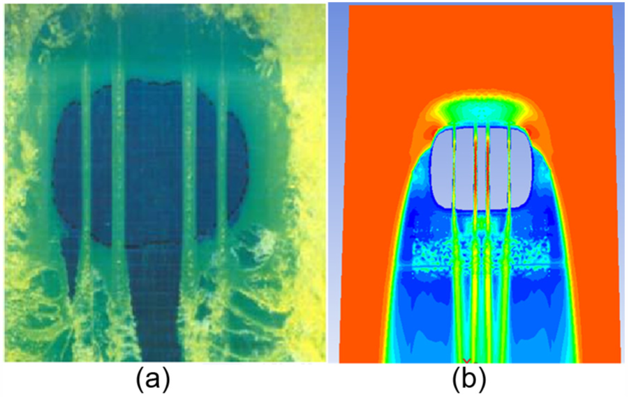
Comparison of simulation and test on water flow: (a) test results and (b) CFD simulation.

The dynamic lift C_L is the vertical force component derived from the water dynamic pressure acts on the tire tread. As shown in Figure 8, C_L was zero before the water contacted the tire tread; at this point, C_L increased sharply, reaching a stable state as the water continued to flow. The faster the speed of the water flows, the greater the dynamic lift C_L and the more likely hydroplaning occur. Based on the conclusion provided by the NASA equation, the hydroplaning occurred once the lift C_L was 2012 N at 80 km/h, and it is nearly equals to half of the tire load and tire hydroplaning occurred.

Figure 8.

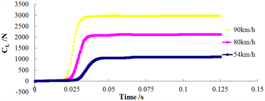
The dynamic lift C_L in different water speed pressure.

In 2001, Okano and Koishi¹⁴ conducted a similar hydroplaning test depicted in Figure 9. In their measurement, several tires with different circumferential grooves were placed on the same car and driven onto a test site at certain acceleration.

Figure 9.

Relationships among the slip ratio, speed, and tread pattern obtained by test.

High-speed photography was used to record the water-flow process. The middle of these test tires in Figure 9 was the same as the simulation tire used in this article. According to the experimental results, hydroplaning occurred when the vehicle reached 82 km/h. The simulation results agreed with the experimental results, which proves that the CFD method used in the simulation can effectively predict hydroplaning speed.

Analysis of water drag for tire grooves with V-riblet bionic non-smooth surfaces

When a tire rolls on wet pavement, the tire-pavement contact area is filled with water and hydroplaning occurs when the dynamic pressure acting on the tread takes the tire off the pavement. The main function of the tread pattern is to drainage water and thereby decreasing dynamic pressure. In other words, the larger the water drainage speed and capacity of the tread pattern, the less possibility of hydroplaning will occur. The frictional resistance and pressure drag created by the unstable water-flow are related to the boundary layer and tread thickness. The drag-reducing principle of a bionic non-smooth surface is to control boundary layer structure and reduce turbulent bursting intensity. Therefore, the V-riblet non-smooth element size can be designed according to boundary layer thickness. The computational details are the same as those in the hydroplaning model described above, with the exception that the bionic V-riblet surface was arranged on the tire pattern groove surface, which is shown in Figure 10.

Figure 10.

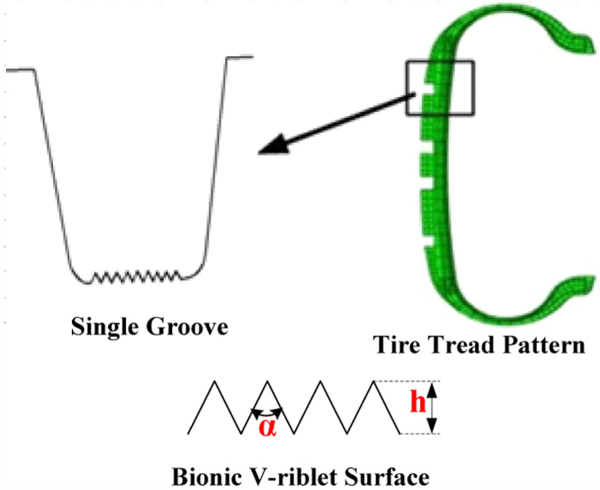
V-riblet surface arranged in grooves.

V-riblet bionic non-smooth surface

The equation for estimating boundary layer thickness is

δ = 0.37 {xR}_{ex}^{- 1 / 5}

(1)

where x is the flow displacement and R_ex is the Reynolds numbers corresponding to x displacement. Per structural parameters, the tread pattern circumferential groove and tire travel speed were fixed between 30 and 120 km/h; and the boundary layer thickness was estimated in the range of 0.6–1.2 mm. To make sure that the non-smooth structure affects the internal structure of the boundary layer, it should not be too close to the thickness of the boundary layer.¹⁹

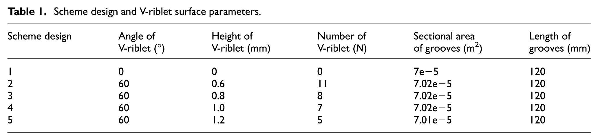
A groove length of 120 mm on the V-riblet non-smooth surface with a 60°angle was chosen to determine the influence of this surface on a tire groove’s water drainage and resistance. Because groove volume affects water resistance, the sectional groove area was kept at 7e−5 m² with a 2.5% range of error. Table 1 presents the scheme design and factors in further detail.

Table 1.

Scheme design and V-riblet surface parameters.

Scheme design	Angle of V-riblet (°)	Height of V-riblet (mm)	Number of V-riblet (N)	Sectional area of grooves (m²)	Length of grooves (mm)
1	0	0	0	7e−5	120
2	60	0.6	11	7.02e−5	120
3	60	0.8	8	7.02e−5	120
4	60	1.0	7	7.02e−5	120
5	60	1.2	5	7.01e−5	120

Mesh of the computational domain

The model size of the longitudinal grooves was 8 mm on the width direction, 9 mm on the depth direction, and 120 mm on the flow direction. The hexahedral and pentahedron grids were combined in a pre-processor software to refine the mesh close to the surface (Figure 11).

Figure 11.

Single-groove mesh and partial enlarge.

Considering fluid viscosity, and in order to make the bionic non-smooth surface disturb the wall viscous sub-layer flow. The dimensionless number of the first grid near the wall is controlled at $y^{+} \leq 5$ . Grid thickness of this first layer near the wall surface can be obtained as follows

y = \frac{μ y^{+}}{C_{μ}^{1 / 4} k_{p}^{1 / 2}}

(2)

where $y^{+}$ is the dimensionless distance to the wall surface, $μ$ is the dynamic viscosity of the fluid, $C_{μ}$ is an empirical constant often taken as 0.09, and k_p is the turbulent kinetic energy of the first node. In addition, when using the SST $k - ω$ model, the number of grid inside the thickness of the boundary layer is at least eight. After repeated attempts, the final grid size of the first layer was 0.01 mm with a growth rate of 1.2 and a maximum computational domain grid size of 0.2 mm.

Calculating boundary conditions

This article focuses on the flowing inlet and outlet boundary as boundary conditions for the computational domain of the V-riblet non-smooth surface.

Inlet conditions: The inlet speed was used to study drag reduction on the V-riblet surface under different flow speeds. Three initial inlet speeds were considered: 22, 25, and30 m/s. The turbulence parameters were calculated according to the fluid theories.

Outlet conditions: Atmospheric pressure was used at the outlet.

Wall boundary conditions: Static and no-slip surfaces were applied to the walls of grooves.

Drainage ability and reduced resistance of V-riblet surface longitudinal groove

Fluid flowing into the longitudinal groove was treated as pipe turbulence fluid. The drag coefficient of this pipe was obtained from empirical or semi-empirical formulas.²⁰

The empirical formula for the drag coefficient of smooth pipe f is

\frac{1}{\sqrt{f}} = 2 \log_{10} (\sqrt{f} R_{e}) - 0.8

(3)

When the fluid reaches the steady state in the tread groove, the numerical testing resistance coefficient can be calculated as follows

f_{smooth} = \frac{8 τ}{ρ {\bar{U}}^{2}}

(4)

where $τ$ is the shear stress (Pa), $ρ$ is the water-flow density (kg/m³), and $\bar{U}$ is the average speed in the groove (m/s).

Table 2 shows the longitudinal groove drag under different flow speeds. The drag coefficient in the longitudinal groove simulation is very close to the drag coefficient calculated using the empirical formula, indicating that turbulence parameters selected by simulation and boundary conditions are reasonable.

Table 2.

The tire free rolling boundary conditions.

Scheme	Speed (m/s)	Wall shear stress (τ, Pa)	$f_{smooth}$	Reynolds (Re)	Empirical formula f
Smooth groove	22	989.9	0.0158	183,915.6	0.0157
	25	1240.9	0.0153	208,995.1	0.0154
	30	1716.8	0.0148	250,794.1	0.0149

Utilizing the Bernoulli equation of steady flow, the following is established

\frac{P_{1}}{ρ g} + z_{1} + \frac{α_{1} v_{1}^{2}}{2 g} = \frac{P_{2}}{ρ g} + z_{2} + \frac{α_{2} v_{2}^{2}}{2 g} + \sum h_{f}

(5)

where $P / ρ g$ is the pressure water head loss (pressure energy), $a v^{2} / 2 g$ is the speed water head loss (kinetic energy), and $α_{1}$ and $α_{2}$ are correction coefficient of kinetic energy of cross section 1 and cross section 2, respectively. Regarding turbulence, $α_{2} = 1$ , laminar flow is $α_{2} = 2$ , and z is water head position (gravity potential energy). The latter is head loss in the water-carrying section between cross section 1 and cross section 2. The tread grooves described here are similar to the straight pipe in the cross section, and the head loss is one way

\sum h = ξ_{c} \frac{L}{d} \frac{v^{2}}{2 g}

(6)

where $ξ_{c}$ represents pipe resistance coefficient; L represents groove length; and d represents the hydraulic diameter of the groove. Using equations (5)–(6), the outlet cross-sectional flow from the entrance is

Q = v_{2} A_{2} = A_{2} \frac{1}{\sqrt{1 + ξ_{c} \frac{L}{d}}} \sqrt{2 g [(\frac{P_{1} - P_{2}}{ρ g}) + \frac{v_{1}}{2 g}]}

(7)

The outlet flow under different schemes in multiple velocities is shown in Table 3. The V-riblet bionic non-smooth surface arranged on the bottom of the grooves led to the highest levels of water displacement, but drainage capacity was inversely proportional to the height of V-riblet surface.

Table 3.

Outlet flow under different schemes in multiple velocities.

Scheme	Speed (m/s)	Outlet flow (kg/m² s)	Change rate (%)
1	22	22,015.5	0
2		22,784.8	3.50
3		22,710.5	3.16
4		22,764.1	3.40
5		22,592.1	2.62
1	25	24,977.5	0
2		25,867.5	3.56
3		25,791.9	3.26
4		25,850.9	3.50
5		25,658.4	2.73
1	30	29,983.5	0
2		31,012.5	3.43
3		30,923.6	3.14
4		30,992.8	3.37
5		30,766.4	2.61

Assuming the evaluation index of the drag-reduction effect, the drag-reduction rate becomes

R = \frac{f_{smooth} - f_{non - smooth}}{f_{smooth}}

(8)

where $f_{non - smooth}$ represents the resistance coefficient of the grooves with V-riblet bionic non-smooth surface. Drag resistance is reduced when R is positive; in other words, the grooves with V-riblet surface drag coefficient are smaller than those of the original smooth grooves. Conversely, drag resistance is increased when R is negative. Without these variables, there is no suitable drag-reduction effect.

Table 4 presents the drag reduction under different water velocities. However, drag-reduction rates decrease as flow velocity increases. Scheme 2 shows three different fluid speeds and maximum outlet flow when it reaches its maximum drag-reduction rate.

Table 4.

Drag reduction under different water velocities.

Scheme	Speed (m/s)	Resistance coefficient	Drag-reduction efficiency (%)
1	22	0.0158	0.0
2		0.0115	27.5
3		0.0122	22.9
4		0.0122	22.6
5		0.0131	17.0
1	25	0.0153	0.0
2		0.0112	26.8
3		0.0119	22.6
4		0.0119	22.3
5		0.0128	16.6
1	30	0.0147	0.0
2		0.0109	26.4
3		0.0115	22.2
4		0.0115	21.9
5		0.0124	16.1

Analysis of drag-reduction mechanism in V-riblet surface

The flow field characteristics of Scheme 2 were chosen for exhibiting the best drag-reducing capabilities to explore the drag-reduction mechanism of the V-riblet surface. A speed of 22 m/s was used with the same smooth wall-flow field characteristics. A flow cross section was chosen 10 mm from the entrance to avoid the impact of the entrance and exit effect. The cross section is shown in Figure 12.

Figure 12.

Characteristic-plane position.

In general, the second vortex group theory and prominent high theory are internationally recognized as accurately representing the bionic theory of resistance and noise reduction.²¹ Flow speed under different drag-reduction effects and increased resistance leads to a decrease in groove surface shear stress within the boundary layer above the groove. This is caused by the effects of the groove tip structure on the boundary layer flow field, which results in a turbulent coherent structure. In this section, analysis of the drag-reduction mechanism in the V-riblet surface is carried out according to the secondary vortex and boundary layer thickness.

Existence of the secondary vortex

Figure 13 shows the contour map of span-wise speed $v_{x}$ on the feature plane where Z = 10 mm. Counter rotating vortex pairs near the tip of the V-riblet surface rotate in opposite directions. The interaction between these counter-rotating vortex pairs and the groove tip caused the ditch inside to produce a small secondary vortex in the opposite direction. The vortex values found in the ditch bottom and tip were opposite values rotating in opposite directions. These counter-rotating vortex pairs weakened groove tip strength, which decreased the effect of the span-wise vortex overshoot and sweeping movement on the groove surface, and restrained the bursts of wall turbulence. The secondary vortex close to the V-riblet surface tip had little influence on the middle-low and groove tip, which also ensures the presence of quiet fluid inside the groove by maintaining the stability of the boundary layer. The increase in quiet regions led to an increase in thickness at the bottom near the wall and a reduction of the speed gradient in this region, therefore reducing the effectiveness of the V-riblet bionic wall friction resistance.

Figure 13.

V_x-speed contour line in the extensional direction: (a) V-riblet non-smooth surface and (b) smooth surface.

Figure 14 shows the contour map of span-wise speed $v_{y}$ on the feature plane Z = 10 mm. Under the groove tip, fluid speed increased, but fluid speed remained relatively low close to the bottom wall region. Both velocities formed a large rotating vortex pair rotating in opposite directions, thus weakening the generation of the horse-shoe vortex fluid in the longitudinal direction and restraining fluid bursts. Thus, the high-intensity turbulent fluid was pushed off the wall and wall resistance was reduced. This change at the bottom of the V-riblet surface in the Y direction was slower than at the tip, which led to a reduction in the speed gradient. This shows that the bottom of the V-riblet surface encouraged low-speed fluid and acted as a lubricant in the movement of external fluid. This caused the external high-speed fluid to pass from the internal low-speed fluid zones, reducing energy loss flowing from the groove wall and reducing drag.

Figure 14.

V_y-speed contour line in the longitudinal direction: (a) V-riblet non-smooth surface and (b) smooth surface.

Speed field analysis

Figure 15 shows a comparison of the speed in the near-wall region of a feature plane Z = 10 mm between the V-riblet model and smooth model. The speed fields within the plane for them have a considerable difference. Mainstream speed was reached within the boundary layer by the speed of the smooth surface in a shorter distance, resulting in a thinner boundary layer and a more intense variation in speed compared to the V-riblet surface. Using the equation $τ = \partial v / \partial y$ , the V-riblet surface wall shear stress within the boundary layer was smaller than that in the smooth wall. This caused the significant decrease in the speed gradient of the V-riblet surface because of the low-speed fluid around the V-riblet. Therefore, drag reduction can be achieved using this bionic V-riblet surface by increasing boundary layer thickness and reducing sticky bottom speed gradients; water drag resistance is reduced and water can flow easily through the tire grooves.

Figure 15.

Comparison of speed distribution in the feature plane Z = 10 mm: (a) V-riblet smooth surface and (b) smooth surface.

Analysis of V-riblet bionic non-smooth surface tire hydroplaning

The optimal V-riblet surface for drag reduction was set on the bottom of the circumferential grooves. According to the tire hydroplaning analysis method provided in chart 3, a comparison was then made between the original smooth tire and the V-riblet bionic non-smooth surface tire. Figure 16 shows the half-tire hydroplaning model arranged with a V-riblet non-smooth structure.

Figure 16.

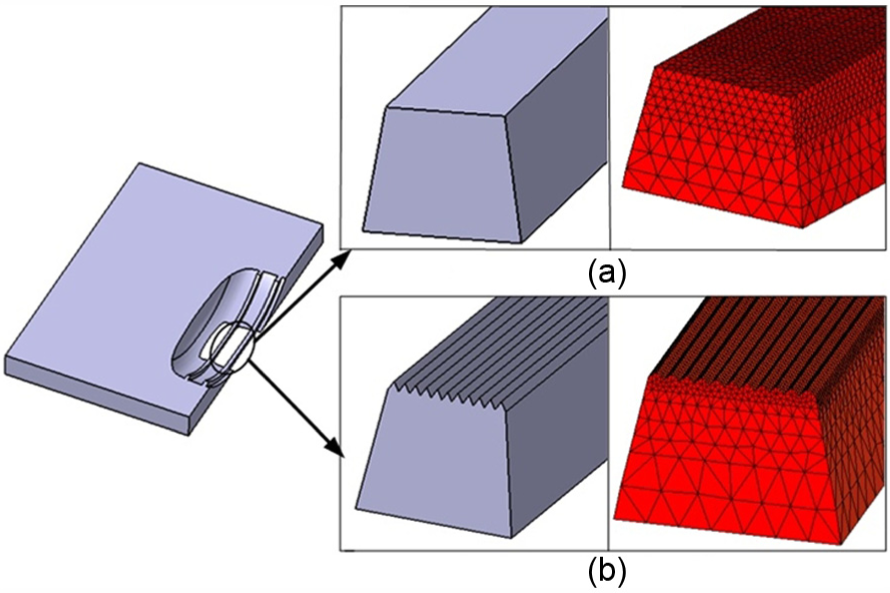
Mesh of tire hydroplaning model: (a) original tire hydroplaning model and (b) V-riblet tire hydroplaning model.

Figure 17 shows the dynamic pressure acting on the tire of the two models with water speeds of 22 and 25 m/s, respectively. When water speed was 22 m/s, the dynamic pressure of the original smooth tire was 202.5 kPa, while that of the V-riblet surface tire was 196.9 kPa. When water speed was 25 m/s, the dynamic pressure of the two models was 264.5 and 255.6 kPa, respectively.

Figure 17.

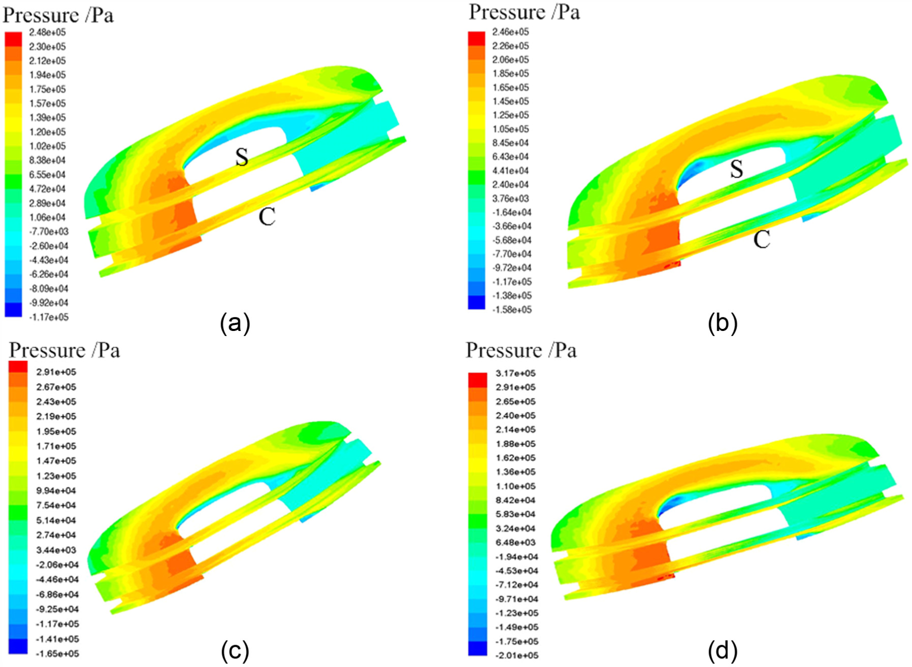
Comparison of dynamic pressure between the original smooth tire and V-riblet surface tire: (a) 22 m/s, smooth surface; (b) 22 m/s, V-riblet surface; (c) 25 m/s, smooth surface; and (d) 25 m/s, V-riblet surface.

According to the equation of dynamic pressure $P = 0.5 ρ V^{2}$ , where V is the speed of water (m/s), ρ is the density of water (1000 kg/m³), and P is the dynamic pressure, hydroplaning speed improved from 1.01 and 1.39 km/h as calculated in the V-riblet bionic non-smooth surface tire with a water-flow speed of 22 and 25 m/s. Water-flow speed was higher, the dynamic pressure of tire grooves arranged with V-riblet bionic non-smooth surface was lower, and its hydroplaning speed was higher.

To investigate the effect of V-riblet bionic non-smooth surface designed in grooves on hydroplaning speed, the water speed within the tire grooves was measured and compared between one tread with smooth grooves and one with non-smooth grooves. Higher flow speed suggests better drainage ability and superior hydroplaning performance. Two measurement lines were selected for both treads: the centroid of the longitudinal grooves (4 mm above the ground) at the (1) tread center and (2) tread shoulder, indicated by C and S, respectively, in Figure 17. Figure 18 demonstrates the results at the water-flow speed of 22 and 25 m/s. It is found that at the same measurement line, the water speed for the V-riblet non-smooth grooves is considerably higher than that of the smooth grooves, which means the V-riblet bionic non-smooth surface tire has better hydroplaning performance.

Figure 18.

Comparison of water speed between the smooth surface grooves and the V-riblet surface grooves at (a) 22 m/s and (b) 25 m/s.

In addition, for the same tread, the flow speed at the center groove is larger than that at the shoulder groove. This is mainly because the water pressure is higher at the center, pushing the water from the center to the shoulder. However, due to the inertia effect, the majority of water goes further away from the shoulder instead of flow into the shoulder groove.

Conclusion

Tire hydroplaning simulation was conducted using the CFD method, and water-flow field characteristics and dynamic pressure acting on the tire can be predicted by the CFD method. From the comparison of hydroplaning speed between the simulation results with the experimental results, it can be concluded that CFD method can effectively predict hydroplaning speed.

The V-riblet bionic non-smooth surface can decrease the speed gradient perpendicular to the direction of the flow along with water drag at the surface. The bottom of the V-riblet surface encouraged low-speed fluid, which acted as a lubricant in external fluid movement resulting in drag reduction. This made the external high-speed fluid to pass from the internal low-speed fluid zones, which reduces energy loss directly flowing from the groove wall, and improves water-flow speed and grooves’ drainage volume, thus reducing the tread hydrodynamic tire pressure when driving on a water-film.

The arrangement of patterned grooves reduces water resistance flowing through the grooves and improves the drainage capacity of grooves. Unlike traditional methods of modifying structure parameters to increase tread grooves void, the design of tread grooves with bionic non-smooth surface can improve hydroplaning performance without increasing tread grooves void volume, which also reduces the tread air-pumping noise caused by grooves large deformation.

Footnotes

Handling Editor: Jose Ramon Serrano

Declaration of conflicting interests

The author(s) declared no potential conflicts of interest with respect to the research, authorship, and/or publication of this article.

Funding

The author(s) disclosed receipt of the following financial support for the research, authorship, and/or publication of this article: This work was supported by the National Natural Science Foundation of China (Grant Nos 51605198 and 51675240), Jiangsu Province Funds for Young Scientists (Grant No. KB2016042722), Six talent peaks project in Jiangsu Province (Project No. JXQC-011) and Road Vehicles in Jiangsu Province Key Laboratory of New Technology Application (BM20082061505).

References

Suzuki

Fujikawa

Improvement of hydroplaning performance based on water flow around tires. SAE paper 2001-01-0753, 2001.

Aksenov

Dyadkin

Gudzovsky

et al . Numerical simulation of car tire aquaplaning. In: ECCOMAS computational fluid dynamics conference, Paris, 9–13 September 1996, pp.815–820. Chichester; New York: Wiley.

Grogger

Weiss

Calculation of the hydroplaning of a deformable smooth-shaped and longitudinally-circumferential grooved tire. Tire Sci Technol 1997; 25: 265–272.

Seta

Nakajima

Kamegawa

et al . Hydroplaning analysis by FEM and FVM: effect of tire rolling and tire pattern on hydroplaning. Tire Sci Technol 2000; 28: 140–156.

Cho

Lee

Sohn

et al . Numerical investigation of hydroplaning characteristics of three-dimensional patterned tire. Eur J Mech A: Solid 2006; 25: 914–926.

Fwa

Pasindu

Ong

GP.

Critical rut depth for pavement maintenance based on vehicle skidding and hydroplaning consideration. J Transp Eng 2011; 138: 423–429.

Wies

Roeger

Mundl

Influence of pattern void on hydroplaning and related target conflicts. Tire Sci Technol 2009; 37: 187–206.

Bushnell

Moore

KJ.

Drag reduction in nature. Annu Rev Fluid Mech 1991; 23: 65–79.

Wang

Yang

Numerical investigation of the passive control of cavity flow oscillations by a dimpled non-smooth surface. Appl Acoust 2016; 111: 16–24.

10.

Zhao

Zheng

et al . Experimental and numerical investigation on drag reduction of non-smooth bionic jet surface. Ocean Eng 2014; 81: 50–57.

11.

Bai

Zhang

Yuan

Numerical analysis of drag reduction performance of different shaped riblet surfaces. Mar Technol Soc J 2016; 50: 62–72.

12.

Fish

Battle

JM.

Hydrodynamic design of the humpback whale flipper. J Morphol 1995; 225: 51–60.

13.

Chen

Rao

Shang

et al . Flow over bio-inspired 3D herringbone wall riblets. Exp Fluids 2014; 55: 1–7.

14.

Okano

Koishi

. A new computational procedure to predict transient hydroplaning performance of a tire. Tire Sci Technol 2001; 29: 2–22.

15.

Zhou

Wang

Ding

et al . Effect of friction model and tire maneuvering on tire-pavement contact stress. Adv Mater Sci Eng 2015; 2015: 632647.

16.

Grogger

Weiss

. Calculation of the three-dimensional free surface flow around an automobile tire. Tire Sci Technol 1996; 24: 39–49.

17.

Zhao

Tan

Zhang

. A high-resolution characteristics-based implicit dual time-stepping VOF method for free surface flow simulation on unstructured grids. J Comput Phys 2002; 183: 233–273.

18.

Dinescu

Hirsch

Leonard

et al . Fluid-Structure Interaction Model for Hydroplan-ing Simulations. SAE Paper 2006-01-1190, 2006.

19.

Sun

Nappo

Mahrt

et al . Review of wave-turbulence interactions in the stable atmospheric boundary layer. Rev Geophys 2015; 53: 956–993.

20.

Chakrabarti

Seidl

Vorwerk

et al . Correlations between porous medium flow data and turbulent tube flow results for aqueous hydroxypropylguar solutions (Part 2). Rheol Acta 1991; 30: 124–130.

21.

Dean

Bhushan

. Shark-skin surfaces for fluid-drag reduction in turbulent flow: a review. Philos T Roy Soc A 2010; 368: 4775–4806.

Numerical investigation of passive control flow to improve tire hydroplaning performance using a V-riblet non-smooth surface