
Abstract
Simulation of engine components enables early design verification and reduced development time while helping racing teams in getting new knowledge. This article presents a multidiscipline dynamic test bench and a benchmark of two different connecting rods for HONDA CRF250R. The test bench embeds mechanical and control system modeling and simulation including electric starters, ignition timing, power control as well as sensors and actuators enabling closed-loop systems. A non-linear finite element program that combines the traditional separate multi-body simulation and finite element modeling and simulation tasks captures all load cases and dynamic effects in one single run. Model reduction techniques are applied to optimize simulation speed and results accuracy. The virtual test bench captures dynamic engine effects and efficiently provides new knowledge about engine performance and integrity.
Keywords
Introduction
More power, reduced weight, and compact dimensions are the main design drivers for racing teams. Due to the hectic racing season, these engines need to be developed within a short time frame. 1 Since the crankshafts, connecting rods, and pistons have a major impact on the integrity and dynamic performance, it is essential that the parts are modeled and benchmarked before the first prototypes are built.2–5 The cyclic engine loads are generally difficult to estimate and model in conventional finite element (FE) programs, and multi-body simulation (MBS) software need to be used for behavior simulation as shown in Johnson et al. 2 and Fleck et al. 4
This approach, as shown in Figure 1, includes many data transfer operations between different modeling and solver environments. The design process is therefore time-consuming and error prone for racing teams with a traditional focus on physical testing. The results can be accurate when there is limited or no interaction between the linear elastic displacements and rigid body displacements. However, this approach has no support for stress stiffening effects introduced by high revolutions per minute (crank speed) (RPM) causing critical tension forces. The MBS + finite element analysis (FEA) approach is therefore best suited for low RPM high torque engines as shown in Johnson et al. 2

The MBS + FEA approach.
Another and more accurate approach for virtual testing of connecting rods is shown in Figure 2. This approach combines “flexible multi-body modeling and simulation.” Some vendors provide a close interfaced MBS/FE solution enabling flexible modes to be used in a MBS simulation. If the engineers know the excitation frequency range and include the right flexible modes, the interaction between rigid body engine dynamics and flexible modes can be captured. The MBS solver calculates the dynamic behavior as well as the amplitudes of the flexible modes which can be used to calculate the physical stresses in a FE program as shown in Johnson et al. 2 and Montazersadgh and Fatemi. 5

The flexible MBS and FEA approach.
This flexible MBS approach is the preference in the aerospace and automotive industry. It is complex to setup and run but has proven to get accurate results when applied by analysts.1,5 However, this approach does not support stress stiffening and the numerical performance can be a challenge when the number of flexible modes increases. Both MBS and FEA approaches can run in parallel with control system software representing the ignition system starters and so on. To capture all inertia loads, identify resonance problems and peak loads at high engine speeds (9000–14,000 r/min), a true integrated non-linear FEA as shown in Figure 3 can provide important benefits.
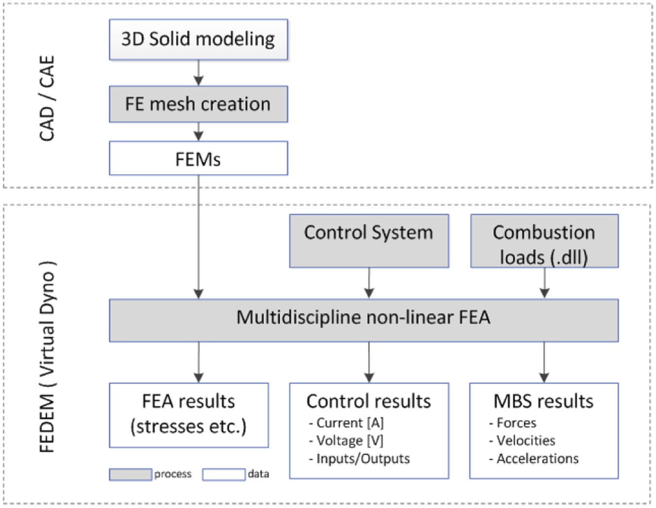
The FEDEM approach.
With an integrated non-linear FEA solver, error prone model and load assumptions can be eliminated. The data transfer problems between incompatible control system, multi-body, and FE solvers are also highly reduced. FE solver benefits like stress stiffening are captured while traditional multi-body gyro and Coriolis effects are preserved by the use of consistent mass matrices and co-rotated frames (one for each engine component). These benefits usually come with longer simulation times, but model reduction techniques can reduce the computational burden without introducing over constrained system problems (ref. MBS).
The authors have therefore developed a dynamic test bench for exact prediction of the dynamic forces, stresses, and displacements that occur in the connecting rod and crankshaft under high-speed operation conditions as described in Vazhappillyn and Sathiamurthi 3 and Montazersadgh and Fatemi. 5 The test bench shown in Figure 4 is based on the Finite Element Dynamics of Elastic Mechanisms (FEDEM) 6 software customized by user functions supporting engine and power control systems as well as post processing features.

The FEDEM test bench.
The article intends to demonstrate the accuracy and significant benefits of the FEDEM test bench (for engines) (FTB) in providing pivotal key performance indicators (KPIs) for the design of the main engine components, with unparalleled short-time processing and simplicity. The article is organized in connecting rod design, method, theory, model, and dynamic simulation and post processing sections. The main connecting rod design drivers are presented including simulation and test challenges. The method section documents why and how a non-linear FE solver can provide important benefits in high-speed engine design and simulation. The theory section addresses the basic modeling, simulation, and post processing fundamentals applied in the proposed dynamic test bench. The model section describes the geometry, FE models, boundary conditions, and loads for a HONDA CRF250R OEM (Original Equipment Manufacturer) engine setup (the reference) and a customized design proposed by MXRR. 7 The simulation section demonstrates the capabilities of the FTB. The modeling process and results are finally discussed and compared to the state-of-the-art MBS and FE capabilities as well as physical dynamometer testing. Modeling and processing times are also considered.
Connecting rod design drivers
When it comes to rod selection and design, “horsepower” and “RPM” are the main design drivers. More power increases the compressive force on the connecting rods while higher RPM increases the tensile forces. In racing, most rods are pulled apart at high RPM. Consequently, in motocross engines running at 14,000 r/min or more, increased tensile strength is the main design driver. High RPM’s also represents critical loads to the crankshaft journal bearings.
The main purpose of the FTB is to integrate traditional separate design and simulation disciplines involved in motocross connecting rod design. These tasks traditionally include the following:
Critical load case identification (MBS) Engine combustion pressure load modeling (compression); Dynamic inertia load identification at high speeds (tension).
Stiffness and mass optimization (reciprocating) Design and analysis (CAD/FEA); Material and manufacturing;
Optimization of fatigue life (shape optimization). Hot spot identification by the use of virtual brittle lacquer (FEA); Strain- or stress-based fatigue analysis (strain gauge outputs); Surface treatment and shape optimization.
Buckling analysis (beam section optimization) Beam section modeling (CAD); Modal analysis (FEA); Buckling load identification (linear and non-linear FEA).
These tasks must be performed to optimize performance and reliability of motocross engine components (structures). Recent advances in predictive virtual analysis tools and methods1,4 have eliminated many problems that would have traditionally been resolved in development test programs. However, tasks (1) and (2) involve the use of multi-body (MBS) and structural software (FEA) which are incompatible and difficult to operate and integrate for most racing teams. These teams have a unique competence in prototyping and testing but only a few have the skills and financial support to buy, learn the simulation software and hardware. The proposed FTB framework should be able to perform a complete design and verification cycle including tasks (1) and (2) in less than 1 h. Buckling analyses (4) as described in Anderson and Yukioka, 8 Moon et al., 9 and Vegil and Vegi 10 are not yet implemented since high-speed motocross engines tend to break in tension due to inertia loads. Fatigue load identification and analysis as shown in Marquis and Solin 11 are implemented in the FTB but not discussed in this article. The design variables in Table 1 can then be redesigned and checked.
FTB design variables.

PD: proportional–derivative; PI: proportional–integral; PID: proportional–integral–derivative; RPM: revolutions per minute (crank speed).
The outputs in Table 2 are predefined as curves and animations in the FTB.
FTB simulation results.

Method
Main FEDEM features
FEDEM is a non-linear FE program embedding control system modeling and simulation. The FEDEM formulation can be optimized for high-speed engine simulation as shown in the next section. Some of the FEDEM features/capabilities applicable to high-speed engine simulations are as follows:
The crankshaft, flywheels, balancing shafts, connecting rods, rockers, cams, piston, and pins are represented by FE models (component mode synthesis (CMS) reduced superelements).
The engine components are connected with various joint types based on numerical robust master and slave techniques eliminating problems with over constrained (rigid body) degrees of freedom that enable more accurate bearing and cylinder/piston modeling. 6
The control systems are created in a two-dimensional (2D) environment interfaced with the three-dimensional engine model. The 2D control systems represent the electric starter and the ignition system controlling the initial crank speed followed by the reciprocating piston pressure causing crankshaft rotation. The control systems also control engine timing, simulation outputs, and the sequence of operations using logical switches.
Modal analysis of the engine assembly at critical speeds can be performed including the effects from stress stiffening. The modes can be animated to identify where the crankshaft of connecting rod need to be strengthen to eliminate resonance or fatigue problems. Fast Fourier transform (FFT) analysis of any type of response curve can be performed to identify the problem in the frequency domain.
Virtual brittle lacquer and S-N curves can be applied to the connecting rod or crankshaft to check how many hours, days, years or duty cycles the engine will survive. Damage plots can be shown to identify the hot spots. Strain gauges can be applied to output strain or stress time histories on known hot spots (saves time compared to full analysis).
These FEDEM features enable the FTB to do dynamic tests and optimization of high-speed engines as shown in Figure 4.
FE model reduction
In dynamic race engine simulation, the stresses, deformations, and vibrations are important to predict since these units are severely loaded compared to stock engines. The geometry and the optimal material properties of the links must be represented by FE models. Each structural component is modeled as a FE superelement with a co-rotated frame for separation of elastic and rigid body displacements. The superelements are based on FE models reduced in FEDEM by the CMS method as shown in equation (1) 6
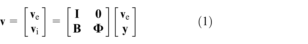
where
In most situations, the internal structural deformations
Dynamic simulation
The external supernode displacements

where

where h is the step length (assumed constant). At time

Subtracting the equations gives
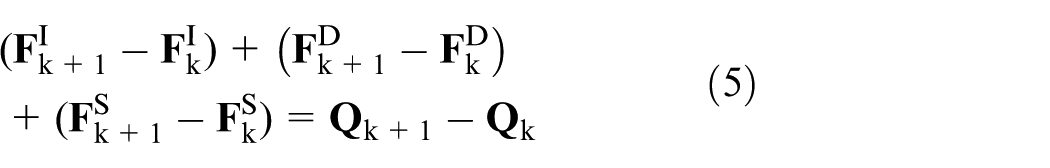
which can be written as

This equation can be expanded to

where
The

The solution at the end of the time increment is used to calculate

which are added to the load increment for the next step

This gives the following approximation for the equation at time step

To achieve equilibrium at the end of the time increment, in the non-linear case, iterations have to be used to minimize the error from the solution. The Newton–Raphson iterations are therefore used to correct by iterations the variables (nodal displacements and modal amplitudes) toward dynamic equilibrium at the time k

Due to the high-speed non-linear connecting rod behavior, the maximum number of iterations was set to 50. The system matrices
With a time step size of 5.0e−05 s, the required number of iterations varied between 2 and 7 for a typical engine test sequence. The sequence included rewing up the engine with an electric motor to the engines power band (3000–9000 r/min) and then running the motor at constant speed in 1 s (150 crank rotations). The total simulation time is about 5 min. When running the engine above 14,000 r/min, the time step was reduced to 1.0e−05 s at the total simulation time increased to 15–20 min.
Model
The main vision with the FTB is to enable race teams to benchmark existing (OEM) engine components against new concepts before they are manufactured and tested in a physical dynamometer. To achieve maximum accuracy of the results, it is essential for the model to be a very precise representation of a real engine and dynamometer. To support easy and direct comparison of two design variants, the main components of two identical engines are modeled and run in parallel. All inputs and outputs are predefined in the FEDEM modeling environment so the only difference will be the actual component to be tested. However, additional outputs can be added and new engine control systems can be added as user functions compiled in a dynamic link library (dll).
The two models shown in Figure 5 are identical HONDA OEM components except for the connecting rods and piston pins. The first model has the steel OEM connecting rod with a steel wrist pin and a stock piston. These components were measured and reengineered in NX and may have minor deviations from the OEM designs, whereas the masses and inertias are exact. The OEM piston, pin and rod were meshed and transferred to the FTB as a Nastran bulk data file. The rod mass was 173 g while the piston and pin masses were 158 (including rings) and 34 g, respectively.

The OEM (right) and MXRR (left) benchmark models.
The MXRR model presents an I-shaped rod design made of a Grade 5 titanium, with aerospace specs. Titanium offers a better stiffness to mass ratio than steel,12–14 which enabled a lower rod mass (125 g). The stock piston was used, but the titanium rod enables the use of a titanium pin with the same stiffness and lower mass (27 g). The total weight saving on the titanium versus the OEM rod was therefore 55 g.
Critical engine loads
Based on the extensive knowledge acquired from top motocross racing teams and engine builders, the authors have formulated a set of loads to cover all possible critical cases.
Load case 1: maximum compression/combustion load
The most critical connecting rod and crankshaft compression loads come from the piston peak pressure and distribution at low engine speeds (<9000 r/min). This load case 1 (LC1) initiates maximum rod compression and crankshaft bending. Maximum rod bending may also come from the compression load but inertia forces can generate higher bending loads in high-speed motocross engines. In motocross engines, the peak pressure typically occurs 10°–13° after top dead center (ATDC). The top dead center (TDC) represents the upper piston and rod position (before ignition). However, the drop in combustion pressure must be considered in order to decide whether this load applies maximum crank torque. Maximum crank torque typically occurs at lower piston pressures and higher ATDC values (20°–30°) depending on the pressure drop (distribution) versus increase in piston leverage. The critical loads causing maximum rod bending and compression as well as crank bending and torque therefore depend on both the cylinder peak pressure and distribution.
In order to simulate with the maximum possible accuracy, all the real inputs targeting the model, the authors decided to implement a complex function to mimic the pressure applied on the dome of the piston during real four-stroke cycles. This approach, combined with the ability to run the model at 14,000 r/min, or above, truly represents an innovation in engine components simulation. The obtained “in-cylinder-pressure” curve is the closest approximation to the real force input occurring in the combustion chamber of this engine.
Three modified statistical Weibull/Gauss functions 15 are implemented in a FEDEM user function to model the pressure distribution during the four piston strokes (intake, compression, power and exhaust). These strokes represent a 720° crankshaft pressure and angular cycle that is reset after four-stroke cycle.
The Gauss functions are scaled by the peak pressure


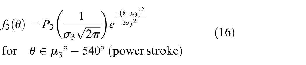
where
The normalized value of
However, when trying to optimize engine performance, the safety margins and structural integrity are sacrificed. By doing “in cylinder pressure” tests, the guesswork is eliminated and the most critical load cases are indirectly identified with minimum uncertainty. Such a test can also identify the intake, and exhaust peak pressures

Typical four-stroke pressure versus crankshaft speed distribution.
The engine performance (power and torque) and hence the peak pressure (


where
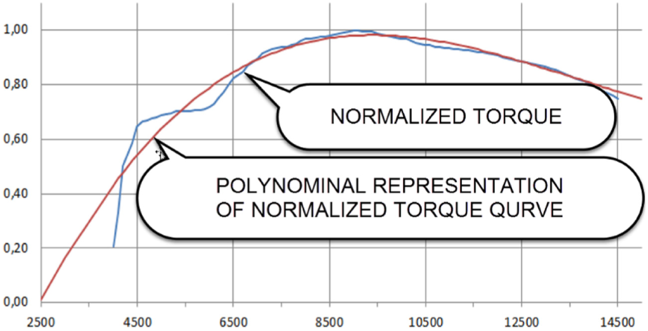
HONDA CRF250R output torque versus RPM.
These parameters can be used to shape the user function until it matches the desired speed-dependent pressure variation. The user function is compiled and linked as a dll located in a FEDEM plugin folder, and it can be used to model the cylinder pressure for all four-stroke combustion engines. The user inputs are shaping the pressure distribution and can be tuned and previewed in an Excel spreadsheet before they are applied to the FTB.
Load case 2: maximum tension load (inertia loads)
The other critical load source is due to the dynamic nature of a slider crank mechanism. High-speed racing engines operating at 14,000 r/min or more are subjected to severe inertia loads from the rotating crankshaft and reciprocating rod, piston, and pin masses. These inertia loads have sometimes proven to be more critical than the combustion pressure loads. All engines also have a rev limiter that cuts the ignition at the maximum allowed speed, which removes the combustion pressure that normally acts damping the critical inertia tension loads. The FTB can model these events to check whether some connecting rod failures are due to fatigue or critical peak loads at maximum speed and ignition cuts.
In most dynamic engine analysis,3,4 the inertia forces are estimated by running separate dynamic load analysis in rigid body (MBS) software. As previously mentioned, this approach is time-consuming and error prone due to numerous data transfer operations. 5 MBS solvers also suffer from limited bearing modeling capabilities due to the rigid body formulation restricting the number of applied joint constrains. Contrary to MBS solvers, the FTB supports stress stiffening effects influencing the dynamic performance and vibration modes at critical speeds/load cases.
In the FTB, the dynamic loads are introduced by the use of a starter engine bringing the crank to the desired test speed or past the minimum operating speed (2500 r/min for the CRF250R as shown in Figure 10). The reference speed is given by a limited ramp function.
The reference speed function is driving the engine up to its power band of 3000–9000 r/min. Then (after e.g. 1.1 s) the engine is started by applying and syncing the piston pressure function described in the previous section (Figure 8). Figure 9 shows that the pressure function described in the previous section is connected to the input block, scaled with the piston area (4633 mm2) to calculate the applied piston force (activated by a logical switch after 1.1 s). Identical electric starter and engine control systems were modeled for the MXRR engine.
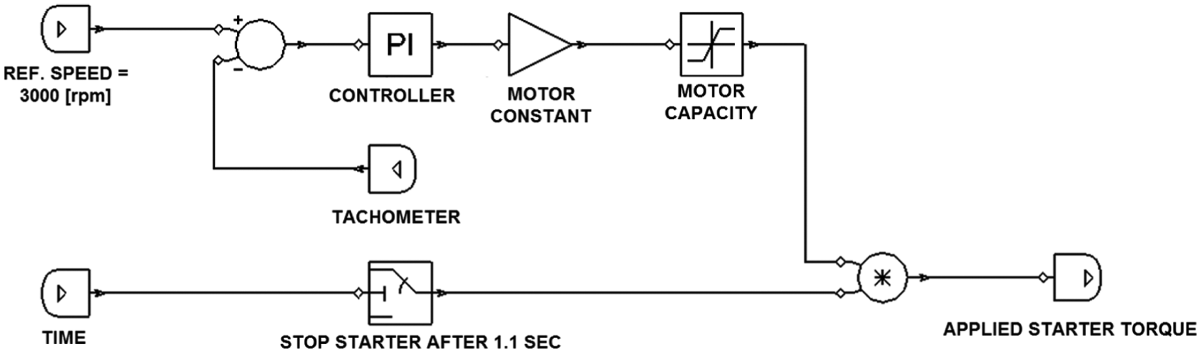
The electric starter control system.
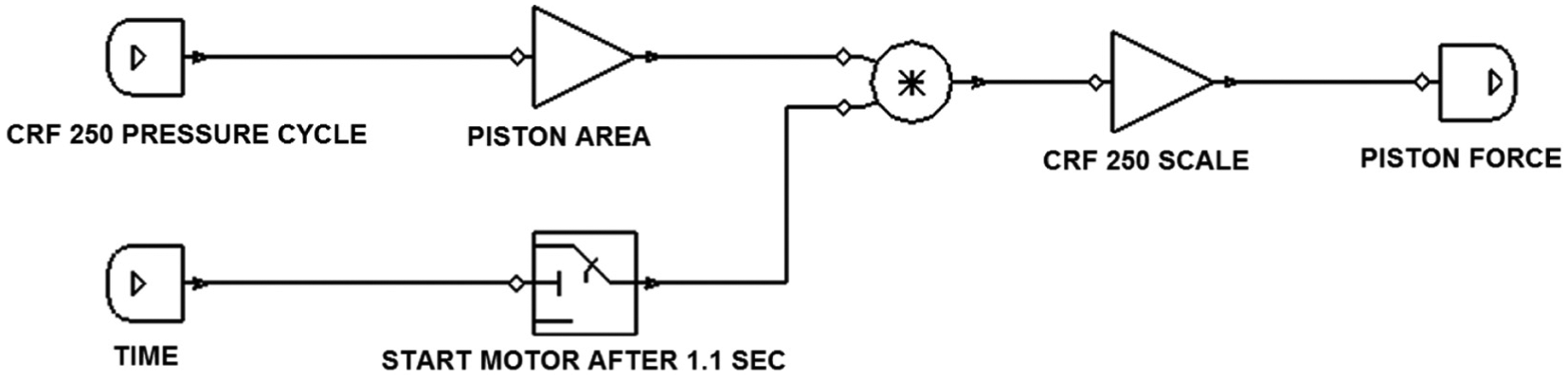
The engine control system.
Simulation setup: combining all load cases in one run
To save modeling and simulation time when benchmarking the OEM and MXRR engine models, load cases 1 and 2 (LC1 and LC2) are combined in one run as shown in Figure 10. The benchmark run can be divided into five different phases:
Electric starter accelerates the crankshaft to 3000 r/min which is within the operating speed range of the HONDA engine.
Combustion starts and accelerates motor to 9000 r/min dynamometer brake is activated to benchmark output torque at 9000 r/min.
Maximum piston compression force and hence output torque are available at 9000 r/min (LC1).
Dynamometer brake is turned off and motor accelerates until rev limiter kicks in at 14,500 r/min which represents maximum tension force (LC2).
Still max throttle but brakes are turned on to bring the RPM down from 14,500 to 8000 in 0.8 s. This event is testing the structural integrity when a bike is airborne and hits the ground while the driver gives max throttle.
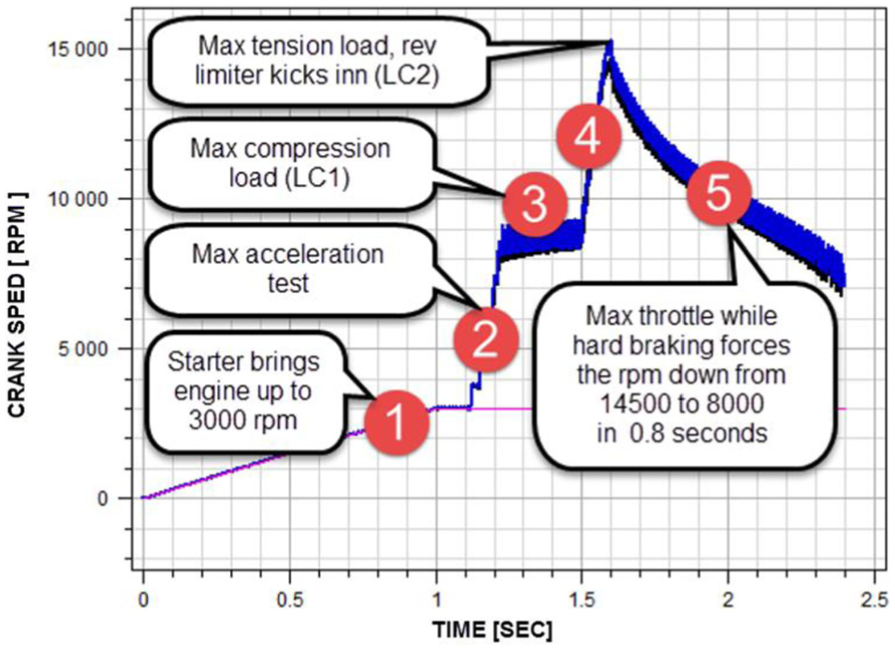
Engine test run.
Phases 3 to 5 capture the worst load cases (LC1 and LC2), while phases 2 and 4 give information about the engine performance. Lighter connecting rods, pins and pistons should reduce the effective crankshaft inertia and hence increase acceleration and throttle response. Before the test run was executed, the crankshafts were balanced in a separate FTB model. Each crankshaft was balanced with a 28% bob weight (
Results and discussions
The key performance indicators (KPIs) shown in Table 3 were chosen for the OEM (steel) and MXRR (titanium) connecting rod benchmark. These performance indicators are related to both performance and structural integrity targets defined in Carlson and Ruff, 16 Lapp et al., 17 and Mian and Carey. 18
Key performance indicators.

OEM: Original Equipment Manufacturer; KPI: key performance indicator.
To qualify the HONDA CRF250R model setup, the piston pressure function (Figure 6) and an output crank damper (dynamometer) were tuned to give the HONDA CRF250R the nominal output break torque and effect of a typical tuned racing engine (31.5 N m and 30 kW at 9000 r/min—stock 24.8 N m and 25.4 kW).
Maximum compression stresses (KPI-1)
Maximum compression stresses for LC1 were expected at 9000 r/min when the engines produce maximum combustion force and output torque. The Von Mises stresses were calculated for all time increments between 1.46 and 1.47 s (phase 3) to capture the stresses at combustion. Maximum compression stress was 631 MPa (MXRR) and 811 MPa (OEM). The 22% peak stress reduction for the MXRR titanium rod is achieved due to a better stiffness-to-mass ratio allowing a more beefy small end section. The average stress level was about 20%–25% lower for the MXRR rod as shown in Figure 11.

LC1—maximum compression stresses (stress range is 0–600 MPa).
The maximum stresses are not acting simultaneously since the two engine speeds are different and hence not synchronized. No bending stresses or deformations indicating buckling problems at maximum piston force (13° after TDC) were observed.
Critical vibration modes (KPI-2)
Modal analysis of the engine assembly was performed at prescribed time incidents in the same run to identify (changes in) vibration modes in simulation phases 2 to 4, for example, the 3000–14,500 r/min speed range (50–240 Hz) (Figure 12). Vibration modes close to 150 Hz is expected to be most critical since they can be excited in phase 3 when maximum piston pressure is applied at 9000 r/min (150 Hz).

Changes in vibration modes due to stress stiffening and non-linear effects.
Four modes were found below 150 Hz but only the fifth (548 Hz) and sixth (561 Hz) modes were related to structural deformation, for example, twisting of the connecting rods and pistons. However, these modes are above the engine bandwidth (240 Hz) and fast Fourier analysis of the big-end bearing loads (KPI-4) did not indicate any responses to modes 5 and 6. These modes are therefore not likely to cause resonance problems unless fluid–structure interactions cause torsional vibrations.
Maximum tension stresses (KPI-3)
Maximum tension stresses for LC2 were expected at 14,500 r/min when the rev limiter kicks in or at maximum speed of 15,200 r/min (MXRR) and 14,700 r/min (OEM) (Figures 13 and 14). The stress variations between 1.58 and 1.62 s were calculated at each simulation time step to capture all peak stresses. Maximum tension stress was 302 MPa (MXRR) and 348 MPa (OEM). These values represent the stress levels when the rods have maximum speed and extensions. The 13% MXRR stress reduction is due to the lower rod and piston pin mass reducing the inertia forces, even though the MXRR top speed is 500 RPM higher. The larger small end section contributes to lower tension stresses. The maximum stresses are not acting simultaneously since the two engine speeds are different and hence not synchronized. No bending stresses or deformations due to inertia forces at maximum speed were observed.

Maximum OEM and MXRR speed.

LC2—maximum tension stresses (stress range is 0–300 MPa).
Big-end bearing loads (KPI-4)
The maximum applied piston combustion force in the vertical stroke direction (x) is 54 kN at 9000 RPM as shown in Figure 15. In a static analysis, this would be the big-end bearing reaction force that would be distributed to the crankshaft journal bearings. However, in the FTB dynamic simulation, the applied piston force is transformed to inertia, damping, and elastic forces. The rods are assigned 3% mass and stiffness proportional damping to eliminate potential internal vibrations and numerical problems at two component modes under 9000 r/min (942 Hz). Energy calculations showed that the applied damping gives the MXRR and OEM rod almost identical damping forces and energy loss. The bearing loads are therefore not sensitive to the applied damping.

Applied piston forces.
Since the MXRR connecting rod has a higher stiffness-to-mass ratio than the OEM solution, the MXRR compression loads are slightly higher as shown in Figure 16. The peak bearing compression loads are 49 kN (MXRR) and 47.5 kN (OEM). However, the peak tension forces due to inertia effects are 9.2 kN (MXRR) and 10.2 kN (OEM). Hence, the peak compression force is 3% higher and the peak tension force is 10% lower for the MXRR rod.
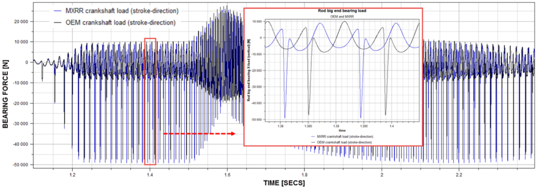
Bearing loads at rod big end.
Axial connecting rod displacements (KPI-5)
Relative sensors are located between the center of the small and big end of the MXRR and the OEM connecting rods. These sensors are measuring the relative axial connecting rod displacement that might influence the compression ratios of the engines. Figure 17 shows that maximum MXRR rod compression is −0.30 mm versus −0.22 mm for the OEM rod. Young’s modulus is higher for the OEM steel rod (2.06e11) compared to the MXRR titanium rod (1.2e11) but higher inertia forces stretching the rod tend to compensate for the higher stiffness. The net effect is more MXRR compression that might cause buckling after combustion, but it will not influence the compression ratio (piston position before ignition).
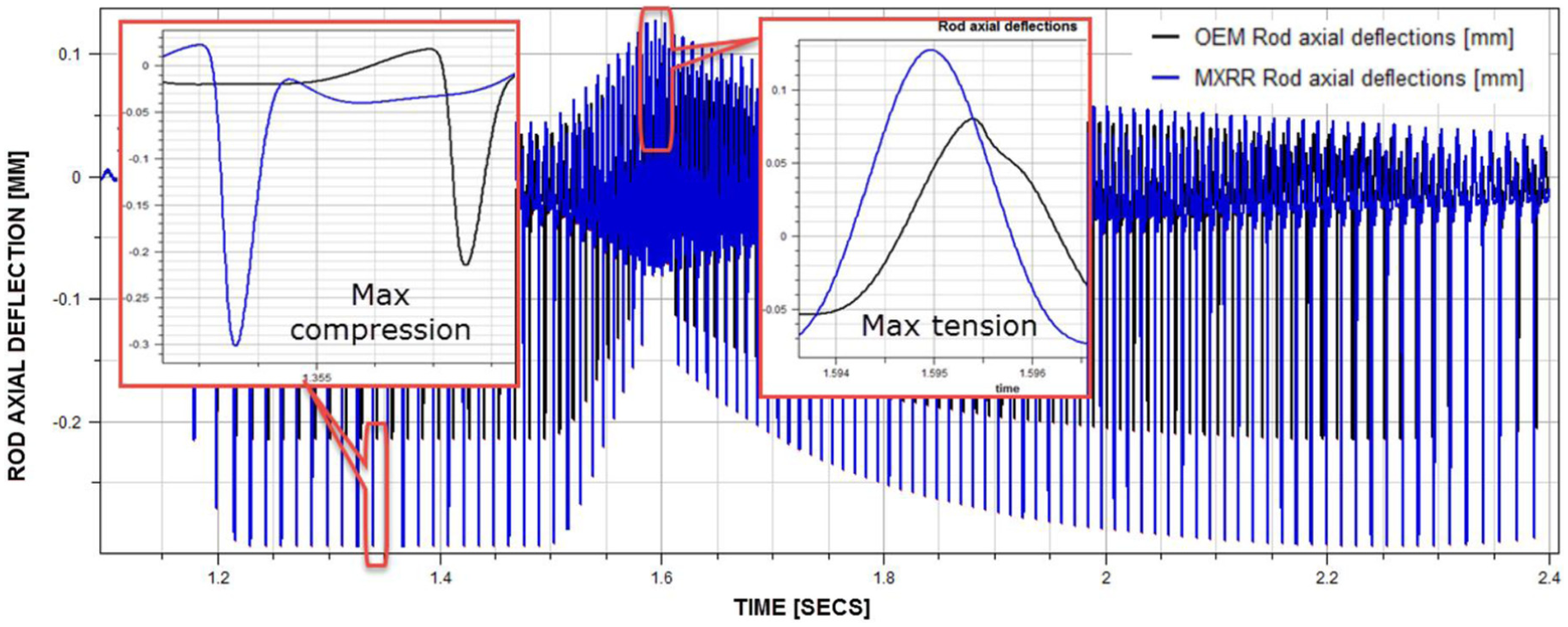
Axial connecting rod displacements.
At constant 9000 r/min (phase 3), the rod extensions are 0.043 mm (MXRR) and 0.033 mm (OEM). At speeds above 14,500 r/min, the MXRR titanium rod extends (0.13 mm) and the OEM rod (0.06 mm). The heavier OEM design causing higher inertia loads, but benefits on a higher Young’s modulus. However, the stretch values after 1.5 s are not directly comparable since the MXRR top speed is 500 r/min higher than the OEM.
Maximum accidental stresses (KPI-6)
This can be regarded as an accidental load case but it is a frequent motocross event. The driver keeps max throttle while the rear tire is hitting ground and hard engine braking occurs. This event is captured in the simulation phase 5 when a “virtual tire breaking” brings the RPM down from 14,500 to 8000 in 0.8 s.
Traditional MBS + FEA approaches applied in Vazhappillyn and Sathiamurthi 3 and Montazersadgh and Fatemi 5 would not capture the worst case time incident without time-consuming data transfer operations and numerous FE analyses. In the FTB software, “virtual brittle lacquer” can be applied to the two connecting rods. Then a worst case stress search can be setup as shown in Figure 18. This feature automatically performs stress analysis of all external element surfaces to identify the peak stresses during simulation phase 5 (1.6–2.4 s). This search identified maximum stresses in phase 5 to be 750 and 925 MPa for the MXRR and OEM connecting rods, respectively, as shown in Figure 19.

Maximum stress search setup.

Maximum accidental stresses (stress range is 0–750 MPa).
Maximum crankshaft acceleration (KPI-7)
This KPI is a performance test on maximum crankshaft acceleration at maximum throttle in simulation phases 2 and 4 (rad/s2) (Figure 20). The rod and piston mass influence the crank inertia and hence the acceleration. The lighter MXRR rod should give a benefit in terms of acceleration and throttle response compared to the OEM design. The top speed will therefore be reached faster with less rod inertia since less effect is needed.

Maximum crankshaft acceleration.
In phase 2, maximum MXRR crankshaft acceleration is in average 5% higher compared to the OEM engine. The difference in acceleration increases up to 9000 r/min due to more available engine torque. In phase 4, the difference is 8%. This is not as obvious since available engine torque drops 20% between 9000 and 14,500 r/min as seen in the HONDA CRF250R torque curve in Figure 7. The MXRR accelerates faster causing a faster drop in available torque which should decrease the difference. However, the OEM reciprocating mass requires more effect to accelerate/decelerate as shown in the KPI-8 section. The net effect is higher engine acceleration for the hole power band when lowering the connecting rod mass.
Kinetic energy and effect variation (KPI-8)
Through FTB, it was possible to clearly demonstrate the importance of minimizing the reciprocating mass of connecting rods. 13 The kinetic energy variations were calculated for the OEM steel and MXRR titanium rods as shown in Figure 21. The kinetic energy was filtered with a 100 Hz low pass filter to remove energy fluctuations and visualize the energy (work) that is required to bring the MXRR (95 J) and the OEM (125 J) connecting rods up to maximum speed (14,500 r/min). Compared to the OEM rod, the MXRR titanium rod requires 24% less energy which has a major impact on the throttle response and gas consumption (Figure 22).

OEM versus MXRR kinetic energy (filtered to the right).

OEM versus MXRR kinetic energy variations.
The energy fluctuations due to the accelerations and retardations of the reciprocating rods are 38 J (OEM) and 27 (MXRR). Less it better because this energy is transmitting to the engine supports causing discomfort and potential fatigue problems. The corresponding effect (power) variations are important because they indicate how much motor effect it takes to accelerate and decelerate the reciprocating rod mass.
The peak power required to accelerate the OEM rod at constant speed (9000 r/min) was 1.1 kW while the MXRR titanium rod only required 0.85 kW (Figure 23). This energy is taken and returned to the crankshaft at TDC and bottom dead center (BDC) and hence not representing a loss in itself. However, due to structural damping and friction effects, the MXRR rod will transmit more output power and less vibrations.

Power variations OEM versus MXRR conrod (engine connecting rod between crank and piston).
Motor power (KPI-9)
Just before 9000 r/min, the dynamometer brake was switched on and the output power was measured for both engines as shown in Figure 24. The left curve shows that the MXRR crank is accelerating faster to 9000 r/min due to less reciprocating mass and hence has a quicker throttle response. The MXRR crank therefore initially produces more output power (1.5 kW). The difference in output power reduces to 0.4 kW when constant speed is reached (the different inertias have no effect).
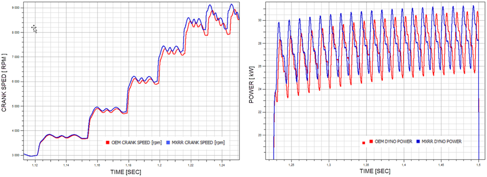
OEM (red) versus MXRR (blue) crank speed and power.
The difference in output power is caused by the difference in reciprocating inertia forces and hence more friction and energy loss for the OEM engine. The difference in output power and top speed will increase with the friction levels and is probably larger that shown in Figure 24. In this benchmark, no friction is applied to the MXRR and OEM pistons or bearings. Both non-linear friction and viscous damping could have been applied but no test data were available. Only 3% Rayleigh (mass and stiffness proportional) damping of the first 2 connecting rod modes was used to cancel out artificial numerical vibrations.
Modeling and simulation performance (KPI-10)
The absolute value of the FTB is to provide engineering knowledge faster and cheaper than real prototyping and testing. Based on numbers from MXRR, a traditional design, production, and dynamometer test process takes between 1 and 2 months depending on the customer requirements.
To shorten this cycle, the FTB has been designed for optimal reuse of input loads, joint constraints, components, and graphs/curves. A FTB design and test iteration will therefore only include manual CAD redesign and FE meshing (1–2 h). Then the meshed FE model is exported to FEDEM as a Nastran bulk data file. Then it can replace an existing engine component in the FTB. The new component will automatically be preprocessed as explained in section “FE model reduction” before a new test run is executed. The model reduction and simulation should take less than 1 h. The simulation setup is robust so a complete redesign and test cycle should take 4–8 h.
Conclusion
This article presents a multidiscipline dynamic test bench (FTB). The test bench embeds electric starters, ignition timing, power control as well as sensors and actuators enabling closed-loop control systems. A FE-based simulation program captures dynamic engine effects which provide new knowledge about engine performance at high speeds (9000–14,500 r/min). Model reduction techniques are applied to optimize the simulation speed and results accuracy. The virtual test bench eliminates the use of rigid body–based solvers (MBS) to identify critical load cases.
To demonstrate the potential of the FTB, steel versus titanium connecting rods for a HONDA CRF250R have been benchmarked. A single test run capturing the most critical load cases is executed. The outputs show the benefits of reducing the reciprocal weight of connecting rods, pistons, and pins. The benefits are reported as 10 different key performance indicators (KPIs) related to both structural integrity and performance. These KPIs are setup as predefined curves and animations to minimize the design and testing cycle for engine components. The FTB has proven to be a robust, accurate, and efficient tool for connecting rod design and testing.
Footnotes
Acknowledgements
The authors would like to thank Fedem Technology AS and Falicon Crankshaft Inc. in providing support and valuable inputs for the article.
Handling Editor: Aditya Sharma
Declaration of conflicting interests
The author(s) declared no potential conflicts of interest with respect to the research, authorship, and/or publication of this article.
Funding
The author(s) received no financial support for the research, authorship, and/or publication of this article.