Sage Journals: Discover world-class research

Abstract

Active control engine mounts notably contribute to ensuring superior effectiveness in vibration suppression. The filtered-x-least-mean-squares algorithm, as a benchmark, is widely implemented for cancelation of disturbing engine vibrations. Such an algorithm requires an accurate secondary path estimate to ensure better performance. This study illustrates that incorporating body input point inertance to the active control engine mount model is necessary when accelerometers are utilized in most practical applications. Secondary path estimation errors caused by neglecting body input point inertance are pointed out via the secondary path modeling mismatch theory. Furthermore, the active control engine mount control system is evolved to fit the acceleration transducer applications. On the basis of the improved active control engine mount control system, a novel extended filtered-x-least-mean-squares algorithm based on the acceleration error signal is proposed to adapt to the extended control system. In the end, severe control collapse of secondary path estimation errors caused by neglecting body input point inertance is verified through simulation. Simulated results are presented to validate the performance of the extended filtered-x-least-mean-squares algorithm based on the acceleration error signal. The study demonstrates that the algorithm produces results showing effective vibration isolation.

Keywords

Active control engine mount body input point inertance secondary path modeling mismatch extended filtered-x-least-mean-squares algorithm acceleration error signal

Introduction

Advanced engine technologies, that is, the variable displacement engine (VDE) or downsizing, put forward increasingly high vibration isolation requirements. Against this background, engine mounts play an important role in depressing vibrations from road inputs and isolating the chassis from high-frequency engine vibrations.¹ Active control engine mounts (ACMs) optimally dampen and isolate the vibrations, noises, and movements generated by a car’s engine in different operating modes. Due to the hydraulic engine mount’s inherent reliability in performance and adaptability to new designs, many researchers consider the hydraulic engine mount (HEM)² as ACM’s cornerstone. Recently, an accurate and precise ACM analytical model has been developed,³ and a current shape control has been discussed in a Maxwell force type actuator for better control.⁴ A linear oscillatory actuator using DC motor was developed for active engine mount in Kobayashi et al.⁵

Various control algorithms have been employed for ACMs. A new robust model reference adaptive control method has been presented for vibration isolation in the presence of uncertainties.^6–8 A combination of adaptive filters and map-based algorithms were developed for improving the tracking behavior during fast engine run-ups in Hausberg et al.⁹ Darsivan et al.¹⁰ investigate using a neurocontroller to reject the disturbance of a plant. A new error-driven minimal controller synthesis (Er-MCSI) adaptive controller has been applied to an active mount with a turbo-diesel engine.¹¹ On average, the filtered-x-least-mean-squares (FxLMS) algorithm is the most widely implemented for active noise and vibration control on adaptive filtering systems due to its stable and predictable operation.^12,13

Such an adaptive control algorithm requires an estimation of the secondary path. It is well acknowledged that the convergence of the least-mean-squares (LMS) algorithm relies on the phase response of the secondary path estimation, exhibiting ever-surging oscillation as the phase increases and ultimately becoming unstable at 90°.¹⁴ However, it is also somewhat distinct that any bias in the estimation of the magnitude of the transfer function could result in an inverse proportional alteration in the maximum stable value of the convergence coefficient.¹⁵

It is common practice to incorporate an acceleration transducer or a load cell at the chassis side to provide an error signal to an adaptive algorithm. In most recent studies,^3,4 the transmitted force to the chassis is often measured as an error signal in a test rig. Experiments with a force transducer are conducted to validate the adaptive controller.¹⁶ However, load cells that are often fixed at the top or bottom sides of the ACM call for more consideration in the process of the actual installation. In practical application, an acceleration transducer is often incorporated into the ACM system instead of the force transducer.¹⁷

The FxLMS algorithm was built upon the force error signal in the most previous engine mount studies.^4,18 The secondary path is changed in the case of adopting acceleration as an error signal in actual application. Control performance can be deteriorated when directly applying the previous algorithm. Thus, this article proposes body input point inertance (IPI) to extend the engine mount model and the FxLMS algorithm. Generally, IPI was developed for calculation of permissible acceleration at all transfer paths;¹⁹ however, there is little consideration for IPI in the process of the ACM system.

In this article, to illuminate the necessity of adding the body IPI transfer function when an accelerometer is installed in a practical ACM system, the research puts emphasis on analytical study of secondary path mismatch and the impact of the body IPI transfer function on the design of the controller. Secondary path estimation errors caused by neglecting body IPI are pointed out by the secondary path modeling mismatch theory. In addition, ACM control system is modified for practical purposes. An extended FxLMS algorithm based on acceleration error signal is proposed for adapting the improved ACM control system. Finally, simulation results are shown to verify the performance of the extended FxLMS algorithm based on acceleration error signal.

Secondary path modeling mismatch of FxLMS algorithm

The influencing parameters of the FxLMS algorithm mainly have two categories that are of concern: influence of the structural system on the stability of the algorithm, where the model of the cancelation path transfer function is exact, and the influence of cancelation path modeling errors upon the stability of the algorithm. The later one will now be discussed in this section. Many researchers^15,20 have pointed out that the optimum weight vectors of the FxLMS algorithm are identical to those of the standard one²¹ as long as the model of the secondary path transfer function is accurate. There are many factors (in particular, the introduction of the secondary path) affecting the stability of the algorithm. Here, the influence of electrical components on the signal’s amplitude and phase and other factors is omitted.

To examine the effects of secondary path estimation errors, a single “estimation error transfer function”H caused by neglecting body IPI will only be introduced as shown in Figure 1. The algorithm is operating in the frequency domain and a single frequency input signal is assumed in this section. For this arrangement, H can be converted from the convolution operations to complex gains. Moreover without loss of generality, the secondary path transfer function is assumed as unity gain and 0 phase.

Figure 1.

Block diagram of FxLMS control with an estimation error transfer function.

Namely, H(k) can be defined by the expression

H (k) = A e^{j θ} = h_{R} + j h_{I}

(1)

where h_R and h_I indicate the real and imaginary part, respectively. The weight vector recurrence formula of the FxLMS algorithm is

\begin{matrix} W (k + 1) = W (k) - 2 μ e (k) \cdot r (k) \\ = W (k) - 2 μ e (k) [H X_{r} (k)] \end{matrix}

(2)

where r(k) is the filter-x signal, X_r(k) is the reference signal, and µ is the convergence coefficient. The error e(k) is defined by the expression

e (k) = d (k) + X_{r}^{T} (k) W (k)

(3)

Equation (2) can be rewritten as²²

W (k + 1) = W (k) - 2 μ H \cdot [P + RW (k)]

(4)

where P is the cross-correlation vector between the primary path signal and the reference vector, and R is auto-correlation matrix of the reference signal. They can be expressed as

\begin{matrix} P = E {d (n) X_{r} (n)} \\ R = E {X_{r} (n) X_{r}^{T} (n)} \end{matrix}

(5)

The optimum weight coefficient vector can be obtained from the steepest descent method

W_{0} = - R^{- 1} P

(6)

The optimum weight coefficient vector is then substituted back into equation (4)

\begin{matrix} W (k + 1) = W (k) - 2 μ \cdot H (- R W_{0} + RW) \\ = W (k) - 2 μ \cdot H R (W - W_{0}) \end{matrix}

(7)

In terms of optimum weight error vector $W_{0}$ , the equation can be restated as

W (k + 1) - W_{0} = W (k) - W_{0} - 2 μ \cdot H R (W - W_{0})

(8)

W' (k + 1) = W' (k) - 2 μ \cdot H RW' (k)

(9)

Since R is symmetric, it can be decoupled by diagonalizing this matrix via an orthonormal transformation

R = Q Λ Q^{T}, Q^{T} = Q^{- 1}

(10)

where $Λ = diag [λ_{1}, λ_{2}, \dots, λ_{n}]$ , and Q is the orthonormal transformation matrix.

Equation (9) can be expressed as

Q^{- 1} W' (k + 1) = Q^{- 1} W' (k) - 2 μ \cdot H Q^{- 1} RW' (k)

(11)

V (k + 1) = (I - 2 μ H \cdot Λ) V (k)

(12)

For this to converge as $k \to \infty$

| 1 - 2 μ H \cdot λ_{i} | < 1

(13)

Expression (13) can be expressed in terms of H real and imaginary parts as

\sqrt{{(1 - 2 μ h_{R} λ_{i})}^{2} + {(2 μ h_{I} λ_{i})}^{2}} < 1

(14)

which can be re-expressed as

μ^{2} λ_{i}^{2} (h_{R}^{2} + h_{I}^{2}) - μ λ_{i} h_{R} < 0

(15)

Thus

0 < μ < \frac{\cos (θ)}{λ_{i} | A |}

(16)

It can be concluded that the effect of overlooking body IPI can be analyzed in two parts, namely, errors in the estimation of the magnitude |A| and phase θ. Magnitude and phase characteristics of body IPI will reduce the size of the maximum convergence coefficient µ. These trends are shown in Figure 2. The upper and lower axes represent the amplitude and phase, respectively. It is illustrated that an error in the estimation of the phase will reduce µ by an amount proportional to $\cos (θ)$ . However, errors in the estimation of the magnitude will reduce the size of the maximum convergence coefficient µ by an amount proportional to the inverse of that error. Furthermore, if the phase change of the body IPI transfer function exceeds 90°, the conventional FxLMS algorithm needs to be modified, thus avoiding divergence.

Figure 2.

The impact on maximum convergence coefficient of magnitude and phase characteristic of body IPI.

As many active vibration control systems do not implement the complex version of the FxLMS algorithm, they perform the algorithm in the time domain. The influence of the secondary path modeling mismatch can also be divided into two categories: errors in the estimation of the magnitude and the phase error. The former will alter the maximum stable value of the convergence coefficient through an inverse proportional relationship which is similar to the complex algorithm. The effect that a phase error has on algorithm stability is more difficult to predict, owing to the alteration of the error induced by the phase errors.¹⁵

Extended ACM control system

The ACM’s lumped parameter model has been greatly improving and developing for years. In this section, the previous ACM model will be developed by adding body IPI in practical application. The developed ACM control system is schematically depicted in Figure 3. The transmitted force signal is converted to the acceleration signal, which is selected as the error signal of the FxLMS algorithm.

Figure 3.

Block diagram of the developed ACM system.

Many researchers have continuously optimized the elastomer model. The Kelvin–Voigt model²³ strongly overestimates both stiffness and damping for higher frequencies. The three-parameter Maxwell model²⁴ resulted in a high-frequency description of stiffness but also in an underestimation of high-frequency damping. On the contrary, the four-parameter model shows good damping and stiffness performance in a relatively high frequency range. These models increase the complicacy and number of parameters to accurately present material properties. Different models have distinct impacts on active dynamic characteristics of ACM and different accurate frequency range, which can be observed in Appendix 2 at length. In view of the accurate description in a large-scale frequency range of the four-parameter model, it is adopted to the ACM model. The dynamic stiffness of the main rubber spring and main rubber bulking property can be expressed in the Laplace domain as

C_{T, Dyn} (s) = c_{T, 1} + \frac{d_{T, 1} c_{T, 2} s + d_{T, 1} d_{T, 2} s^{2}}{c_{T, 2} + (d_{T, 1} + d_{T, 2}) s}

(17)

C_{B, Dyn} (s) = c_{B, 1} + \frac{d_{B, 1} c_{B, 2} s + d_{B, 1} d_{B, 2} s^{2}}{c_{B, 2} + (d_{B, 1} + d_{B, 2}) s}

(18)

This article incorporates the model of Hausberg into the ACM controller to analyze the FxLMS algorithm’s control performance. All specific deduction can be obtained from Appendix 3. The transmitted force to the body F_T can be written as³

F_{T} (s) = K_{Dyn} (s) \cdot X_{T} (s) + S_{Dyn} (s) \cdot U (s)

(19)

The primary path transfer function K_Dyn and the secondary path transfer function S_Dyn are expressed as in equations (20) and (21)

K_{Dyn} (s) = \frac{F_{T} (s)}{X_{T} (s)} = c_{T, Dyn} (s) + \frac{{A_{T}}^{2} - \frac{m_{A} A_{A} A_{T}}{C_{A, Dyn} (s)} s^{2}}{\frac{{A_{B}}^{2}}{C_{B, Dyn} (s)} + \frac{{A_{K}}^{2}}{C_{K, Dyn} (s)} + \frac{{A_{A}}^{2}}{C_{A, Dyn} (s)}}

(20)

\begin{matrix} S_{Dyn} (s) = \frac{F_{T} (s)}{U (s)} \\ = - \frac{k_{M} ((\frac{{A_{B}}^{2}}{C_{B, Dyn} (s)} + \frac{{A_{K}}^{2}}{C_{K, Dyn} (s)}) m_{A} s^{2} + A_{A} A_{T})}{(R + Ls) C_{A, Dyn} (\frac{{A_{B}}^{2}}{C_{B, Dyn} (s)} + \frac{{A_{K}}^{2}}{C_{K, Dyn} (s)} + \frac{{A_{A}}^{2}}{C_{A, Dyn} (s)})} \end{matrix}

(21)

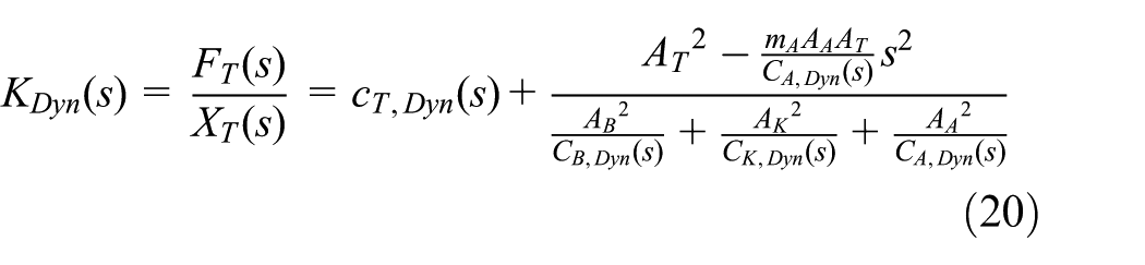
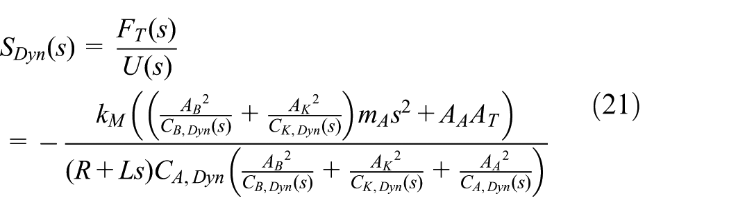
where C_A,Dyn(s) and C_K,Dyn(s) can be described as

C_{A, Dyn} (s) = m_{A} s^{2} + (d_{A} + \frac{k_{M}^{2}}{R + Ls}) s + c_{A}

(22)

C_{K, Dyn} (s) = m_{K} s^{2} + d_{K} s

(23)

Equation (21) gives the accurate secondary path function and is essential for the FxLMS control system. In practical implementation, it is acknowledged that the secondary path is estimated as a finite impulse response (FIR) filter.

The natural frequency of the ACM system can be obtained by analyzing the characteristic poles of the above transfer paths. For a typical active HEM, the transfer behavior of the ACM is dominated in the lower frequency (<25 Hz) by the dynamics of the fluid channel and in the frequency range above 25 Hz the fluid channel is hydraulically closed. Under this assumption, two complex conjugate poles are analytically identified³

s_{p, 1}^{2} = - \frac{A_{K}^{2}}{(\frac{A_{B}^{2}}{c_{B, 1}} + \frac{A_{A}^{2}}{c_{A}}) m_{K}}

(24)

s_{p, 2}^{2} = - \frac{(\frac{A_{B}^{2}}{c_{B, 1}} + \frac{A_{A}^{2}}{c_{A}}) c_{A}}{\frac{A_{B}^{2}}{c_{B, 1}} m_{A}}

(25)

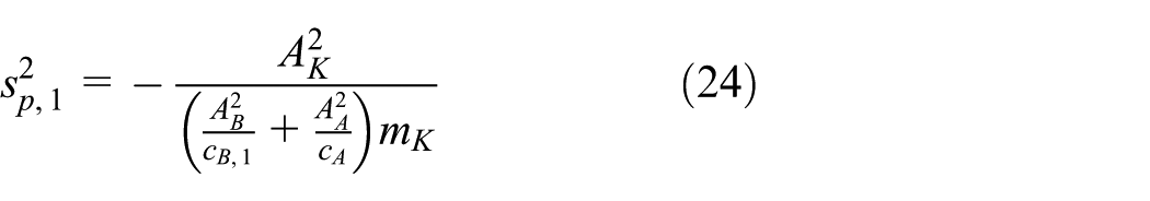
This two conjugate poles correspond to the natural frequency of the ACM system. The first one is dominated by the mass in the fluid channel and the second is referred to as the actuator’s resonance frequency. Substituting the parameters in Appendix 4 into the above equation, the natural frequency of the mass in fluid channel is 9.21 Hz and the actuator’s resonance frequency is 211 Hz.

On the basis of the previous linear lumped parameter model, body IPI function is introduced to integrate the ACM control system depicted in Figure 4. With regard to obtaining the reference signal X_r(n), the engine speed w_e obtained from a crankshaft tachometer and multiplied by the engine’s main order r will be implemented. In this case, the reference signal is given by

X_{r} (n) = e^{j w_{e} rTn}

(26)

where T is the sample time, $r = 2$ for a four-cylinder engine in this study.

Figure 4.

Implementation of adding body IPI in ACM model.

The transmitted force to the body which is difficult to measure directly is converted to the acceleration signal after introducing the body IPI. The acceleration signal is conducted as an error signal. The definition of IPI can be written as follows

H_{a / F} (ω) = \frac{\overset{\cdot\cdot}{X}}{F}

(27)

where $\overset{\cdot\cdot}{X}$ is the indicator acceleration, F is the force, and $ω$ is the angular frequency.

Generally, the acceleration transfer function can be achieved by the finite element method or an experimental test. Figure 5 shows how to obtain it by impact testing.²⁵

Figure 5.

Schematic diagram of body IPI measurement.

Extended FxLMS algorithm based on acceleration error signal

In an extended ACM system, the acceleration signal, rather than the transmitted force, is treated as the error signal. Therefore, in order to avoid diminishing the control performance caused by the secondary path modeling mismatch, the conventional FxLMS needs to be modified. The original “filtered” reference signal can be expressed as follows²²

r (n) = X_{r}^{T} (n) S_{Dyn} (n)

(28)

where $X_{r}^{T}$ is the reference signal. Here, it is expressed as a vector

R (n) = [r (n), r (n - 1), \dots, r (n - L + 1)]^{T}

(29)

And the error criterion can be expanded as follows

e (n) = f_{1} (n) + R^{T} (n) \cdot W (n)

(30)

where f₁(n) is the transmitted force from the primary path. In actual system implementation, the weight coefficient vector is often updated according to the gradient descent algorithm

W (n + 1) = W (n) - μ \cdot \nabla

(31)

\nabla \approx \hat{\nabla} = \frac{\partial e^{2} (n)}{\partial W} = 2 e (n) R (n)

(32)

where µ is the convergence coefficient. Iterative formula of weight coefficient vector is

W (n + 1) = W (n) - 2 μ e (n) R (n)

(33)

Now, assume the body IPI function as H_a/F(n), the “filtered” reference signal needs to be updated as follows

r' (n) = r (n) H_{a / F} (n)

(34)

Then it can be described as a vector

R' (n) = [r' (n), r' (n - 1), \dots, r' (n - L + 1)]^{T}

(35)

Then transmitted force error signal e(n) is converted to the acceleration error $e' (n)$ and can be expanded as

e' (n) = {f_{1}}^{T} (n) H_{a / F} (n) + R^{'} (n)^{T} \cdot W (n) = e (n) H_{a / F} (n)

(36)

Differentiating this with respect to the weight coefficient vector gives

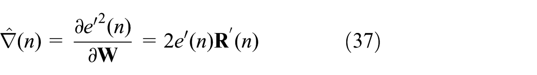
\hat{\nabla} (n) = \frac{\partial {e'}^{2} (n)}{\partial W} = 2 e' (n) R^{'} (n)

(37)

Iterative formula of weight coefficient vector is rewritten as

W (n + 1) = W (n) - 2 μ e' (n) R^{'} (n)

(38)

Comparing equations (38) and (33), it is found that the “filtered” reference signal and error signal have changed. When the force error signal is converted into acceleration error signal, the secondary path estimation ${\hat{S}}_{Dyn} (n)$ needs to be modified with adding body IPI estimation depicted in Figure 6. Practical implementation of the extended FxLMS algorithm is illustrated with a Simulink representation in Appendix 4.

Figure 6.

Block diagram of extended FxLMS algorithm.

In a practical implementation of FxLMS, it is necessary to introduce tap leakage to prevent problems with digital overflow of weight values as a result of quantization errors. Besides minimizing the mean square error, the minimization of the magnitude of the weights coefficients is also conducted. The error criterion can be re-expressed as follows²⁶

minimize ({e'}^{2} (n) + \frac{α}{2} {‖ w (n) ‖}^{2})

(39)

With this modified error equation, the gradient expression of equation (37) becomes

\hat{\nabla} (n) = \frac{\partial ({e'}^{2} (n) + \frac{α}{2} {‖ W (n) ‖}^{2})}{\partial W} = 2 e' (n) R^{'} (n) + α W (n)

(40)

Iterative formula of weight coefficient vector is derived as follows

W (n + 1) = (1 - α μ) W (n) - 2 μ e' (n) R^{'} (n)

(41)

This addition of tap leakage to the FxLMS algorithm will bound the weight coefficients and hence preventing overflow. However, it can increase the value of minimum mean square error. The selection of leakage coefficient α should take these two effects into account. In general, αµ is often of one or two bits of the algorithm calculation word length.

Simulation results and discussion

Imposing unit steady state excitation varied with frequency in the body connecting point, and acceleration response in line with the direction of the exciting force can be acquired, thus obtaining the curves of IPI of the active control engine mounting points. By means of experimental testing, the body IPI curves of front and rear mount can be obtained, as shown in Figure 7. The acceleration response of the red line reaches the peak at the frequency of around 220 Hz, while the green one reaches the peak at almost 370 Hz. It is noted that the vibration response is much remarkable at the peak frequency. Two representative body IPI curves are selected for algorithm validation. There is a dramatic fluctuation in the phase of the rear mount and body while there is a few change in the second one. In the previous study, amplitude–frequency characteristics have long been a focus topic in the transfer path analysis (TPA) and other areas. There is little attention on the phase–frequency characteristics. In this section, phase information is important to the stability of the algorithm.

Figure 7.

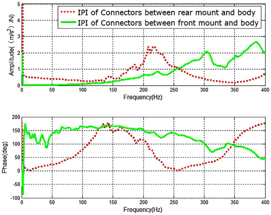
Body IPI curves of connectors between mount and body.

The phase error of the secondary path estimation, as well as the body IPI function, can bring severe instability to the control algorithm. Before investigating the performance of the extended FxLMS algorithm based on the acceleration error signal, precise secondary path estimation needs to be given high priority, thus excluding the phase error caused by the secondary path estimation. It is an idiomatic way to model the estimation of the secondary path as an FIR filter. A 150 taps FIR is applied to match the secondary path, and good consistency is shown in Figure 8.

Figure 8.

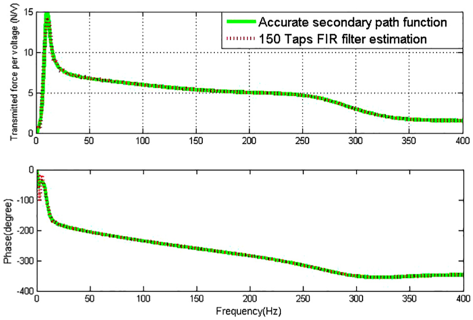
The active dynamic characteristic of the secondary path estimation.

In order to demonstrate the impact of adding the body IPI transfer function on control performance, the conventional FxLMS control performance is validated and compared with the uncontrolled one. The input excitation of engine vibration is simulated as a sinusoidal signal with 0.1 mm in amplitude. The sine sweeping frequency range is 0–400 Hz and sweeping rate is 60 Hz/min. Active control of the ACM comes into action only after 20 Hz, which is consistent with four-cylinder engine main firing order frequency at idle. The LMS adaptive filter length is 50 in the MATLAB. The step size of the LMS adaptive filter has to be small enough to prevent the instance of the conventional FxLMS algorithm failing to function due to the unreasonable step size. It is 0.000001 here. According to Figure 9, acceleration at the connecting point of the mount and body has been remarkably reduced after controlled, contrary to noncontrolled circumstance. Nevertheless, the control effects gradually lessen after 105.4 s. Furthermore, as the phase of the acceleration frequency response exceeds 90° at almost the same time, the conventional FxLMS algorithm fails to function.

Figure 9.

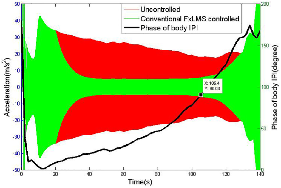
Conventional FxLMS algorithm control performance.

In order to adapt the body IPI transfer function, the performance of the proposed extended FxLMS algorithm is studied and validated compared with the uncontrolled condition. All the simulation settings are the same as the process of the conventional FxLMS algorithm. When Figure 9 is compared with Figure 10, acceleration at the connecting point of the mount and body has been remarkably reduced even if the phase of the acceleration frequency response exceeds 90°.

Figure 10.

Extended FxLMS algorithm control performance.

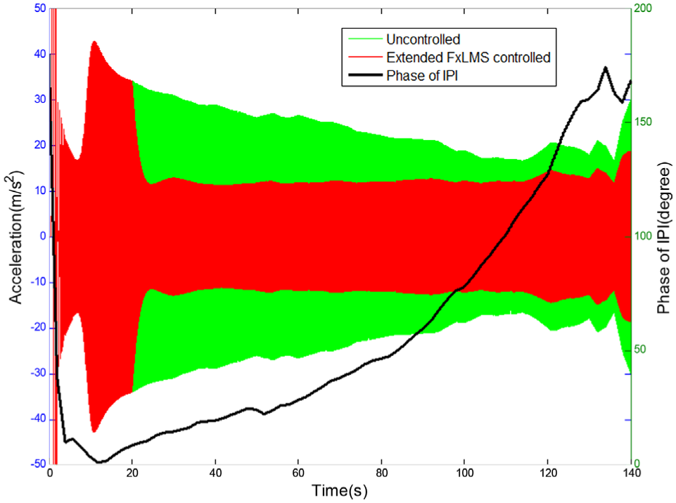
The conventional FxLMS algorithm fails to inhibit engine vibration once the phase of body IPI transfer function exceeds 90°. However, the extended FxLMS algorithm based on acceleration error signal reveals effective performance and stability regardless of the behavior of body IPI. The LMS adaptive filter length is 50 and the step size is 0.00005. The body side acceleration of the rear mount and front mount in the time domain is shown in Figures 11 and 12, respectively. From the figures, a dramatic reduction in the time domain of the transmitted acceleration to the chassis is clearly shown. The acceleration in both two conditions has decreased by 80% at most of the time. There is still a reduction of 30% even in the 300 s in Figure 11.

Figure 11.

Time domain response of acceleration on the rear mount.

Figure 12.

Time domain response of acceleration on the front mount.

As a measure for vibration isolation performance of the ACM, dynamic stiffness is calculated as shown in Figures 13 and 14. Notably, the dynamic stiffness of the ACM with the extended control algorithm is significantly reduced compared with that of the uncontrolled one over the frequency ranges of control.

Figure 13.

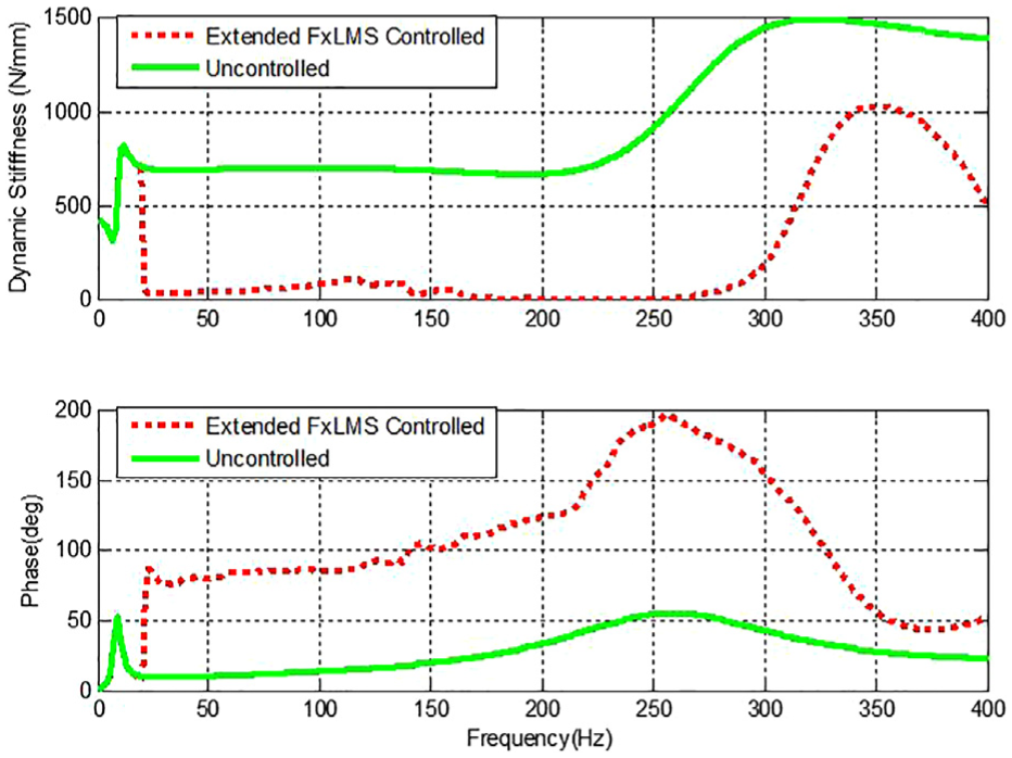
Dynamic stiffness of the rear mount after extended FxLMS control.

Figure 14.

Dynamic stiffness of the front mount after extended FxLMS control.

Conclusion

In this study, it’s shown that the acceleration sensor is often incorporated into the ACM system instead of the force transducer in practical application. To adapt to the demands of actual condition, an extended ACM control system is developed and improved. Body IPI function is introduced to integrate the ACM system. It is mathematically proven by the secondary path modeling mismatch theory that overlooking body IPI can result in a severe control problem. It is validated that the conventional FxLMS algorithm fails to function once the phase of the acceleration frequency response exceeds 90°.

To avoid devastating the control performance caused by the secondary path modeling mismatch of adding body IPI transfer function, the extended FxLMS algorithm, based on the acceleration error signal, is proposed. By means of experimental testing, the body IPI curves of front and rear mount are acquired. It is concluded that the acceleration in both two engine mounts has decreased by 80% at most of time domain after applying the extended algorithm. The dynamic stiffness of the rear and front mount has been decreased to almost zero at most frequency range. The extended FxLMS algorithm shows effective capability and easy access to implementation in the engineering application.

Footnotes

Appendix 1

Appendix 2

Applying the three main rubber models into the whole ACM model, the active dynamic characteristics can be obtained to examine the elastomer models’ validity and applicability, which are shown in Figure 15. It’s obvious that the four-parameter model has an accurate description in a relative large scale frequency range.

Appendix 3

The equations of the ACM system are derived as follows. All the specific structure parameters originate from Table 1. Figure 16 illustrates the lumped parameter model.

The bulking property of the main rubber spring can be obtained by the following equation

(42)

- P (t) A_{B} = C_{B, Dyn} x_{B}

where P(t) is the pressure in upper chamber.

Under the assumption that the fluid is incompressible, the continuity equation is expressed as follows

(43)

A_{T} {\overset{\cdot}{x}}_{T} = A_{A} {\overset{\cdot}{x}}_{A} + A_{K} {\overset{\cdot}{x}}_{K} + A_{B} {\overset{\cdot}{x}}_{B}

where x_T is the displacement at the engine side, x_A is the actuator displacement, and x_K is the displacement of fluid in the inertia track.

The fluid equation in inertia track connecting the upper chamber to the lower chamber can be written as follows

(44)

- A_{K} P (t) = m_{K} {\overset{\cdot\cdot}{x}}_{K} + d_{K} {\overset{\cdot}{x}}_{K}

The actuator is taken into account as a mass–spring–damper system, acting on the diaphragm. The equation can be expressed as follows

(45)

f_{A} (t) - A_{A} P (t) = m_{A} {\overset{\cdot\cdot}{x}}_{A} + d_{A} {\overset{\cdot}{x}}_{A} + c_{A} x_{A}

where f_A is the actuator force. A coil actuator complies with the Lorentz–Force Principle and an electrical circuit equation of the moving coil actuator can be obtained according to the second law of Kirchhoff, as shown, respectively

(46)

f_{A} = Bli = k_{M} i

(47)

U = Ri + L \frac{di}{dt} + k_{M} {\overset{\cdot}{x}}_{A}

where U is the control voltage. Eventually, the force transmitted to the chassis consists of three parts: the transmitted force from the main rubber F_T₁, the transmitted downforce from the mount structure brace F_T₂, and the actuator’s force transmitted to the base F_T₃, as shown in Figure 17.

The total transmitted force to the chassis can be expressed as follows

(48)

\begin{matrix} F_{T} = F_{T 1} + F_{T 2} + F_{T 3} \\ = C_{T, Dyn} x_{T} - P (A_{T} - A_{A}) + c_{A} x_{A} + d_{A} {\overset{\cdot}{x}}_{A} - f_{A} \\ = C_{T, Dyn} x_{T} - P A_{T} - m_{A} {\overset{\cdot\cdot}{x}}_{A} \end{matrix}

Appendix 4

Academic Editor: Mario L Ferrari

Declaration of conflicting interests

The author(s) declared no potential conflicts of interest with respect to the research, authorship, and/or publication of this article.

Funding

The author(s) disclosed receipt of the following financial support for the research, authorship, and/or publication of this article: This work was supported by the National Natural Science Foundation of China (grant number 51205290) and the Fundamental Research Funds for the Central Universities (grant number 2016).

References

Akanda

Adulla

Application of evolutionary computation in automotive powertrain mount tuning. Shock Vib 2006; 13: 85–102.

Tikani

Vahdati

Ziaei-Rad

Two-mode operation engine mount design for automotive applications. Shock Vib 2012; 19: 1267–1280.

Hausberg

Scheiblegger

Pfeffer

et al . Experimental and analytical study of secondary path variations in active engine mounts. J Sound Vib 2015; 340: 22–38.

Lee

CW.

Model based feed-forward control of electromagnetic type active control engine-mount system. J Sound Vib 2009; 323: 574–593.

Kobayashi

Hirata

Kitayama

Proposal of linear oscillatory actuator using DC motor for active control engine mount. Int J Appl Electrom 2016; 52: 1647–1653.

Fakhari

Choi

Cho

CH.

A new robust adaptive controller for vibration control of active engine mount subjected to large uncertainties. Smart Mater Struct 2015; 24: 045044.

Fakhari

Ohadi

Talebi

HA.

A robust adaptive control scheme for an active mount using a dynamic engine model. J Vib Control 2013; 21: 2223–2245.

Fakhari

Ohadi

Robust control of automotive engine using active engine mount. J Vib Control 2013; 19: 1024–1050.

Hausberg

Plöchl

Rupp

et al . Combination of map-based and adaptive feedforward control algorithms for active engine mounts. J Vib Control. Epub ahead of print 20 January 2016. DOI: 10.1177/1077546315626323.

10.

Darsivan

Martono

Faris

WF.

Active engine mounting control algorithm using neural network. Shock Vib 2009; 16: 417–437.

11.

Hillis

Harrison

AJL

Stoten

DP.

A comparison of two adaptive algorithms for the control of active engine mounts. J Sound Vib 2005; 286: 37–54.

12.

Das

Moreau

Cazzolato

BS.

A computationally efficient frequency-domain filtered-X LMS algorithm for virtual microphone. Mech Syst Signal Pr 2013; 37: 440–454.

13.

Qiu

Lee

et al . A multi-resolution filtered-x LMS algorithm based on discrete wavelet transform for active noise control. Mech Syst Signal Pr 2016; 66–67: 458–469.

14.

Morgan

DR.

History, applications, and subsequent development of the FXLMS Algorithm [DSP History]. IEEE Signal Proc Mag 2013; 30: 172–176.

15.

Snyder

Hansen

CH.

The effect of transfer function estimation errors on the filtered-x LMS algorithm. IEEE T Signal Proces 1994; 42: 950–953.

16.

Lee

CW.

Dynamic analysis and control of an active engine mount system. Proc IMechE, Part D: J Automobile Engineering 2002; 216: 921–931.

17.

Römling

DIS

Vollmann

DIFS

Kolkhorst

DIT.

Active engine mount system in the new Audi S8. MTZ Worldw 2013; 74: 34–38.

18.

Nakaji

Satoh

Kimura

et al . Development of an active control engine mount system. Vehicle Syst Dyn 1999; 32: 185–198.

19.

Baik

Jung

Kang

. The study on the optimization of attachment stiffness in vehicle body. SAE technical paper 2007-01-2346, 2007.

20.

Boucher

Elliott

Nelson

PA.

Effect of errors in the plant model on the performance of algorithms for adaptive feedforward control. IEE Proc: F 1991; 138: 313–319.

21.

Widrow

Steams

SD.

Adaptive signal processing. Englewood Cliffs, NJ: Prentice Hall, 1985.

22.

Tobias

Bermudez

JCM

Bershad

NJ.

Mean weight behavior of the filtered-X LMS algorithm. IEEE T Signal Proces 2000; 48: 1061–1075.

23.

Mansour

Arzanpour

Golnaraghi

Design of a solenoid valve based active engine mount. J Vib Control 2012; 18: 1221–1232.

24.

Sjöberg

Kari

Non-linear behavior of a rubber isolator system using fractional derivatives. Vehicle Syst Dyn 2002; 37: 217–236.

25.

Guo

Qiu

et al . Transfer path analysis and control of vehicle structure-borne noise induced by the powertrain. Proc IMechE, Part D: J Automobile Engineering 2012; 226: 1100–1109.

26.

Cioffi

SJ.

Limited-precision effects in adaptive filtering. IEEE T Circuits Syst 1987; 34: 821–833.

Extended filtered-x-least-mean-squares algorithm for an active control engine mount based on acceleration error signal

Abstract

Keywords

Introduction

Secondary path modeling mismatch of FxLMS algorithm

Extended ACM control system

Extended FxLMS algorithm based on acceleration error signal

Simulation results and discussion

Conclusion

Footnotes

Appendix 1

Appendix 2

Appendix 3

Appendix 4

Declaration of conflicting interests

Funding

References