Sage Journals: Discover world-class research

Abstract

The purpose of this article is to analyze various wind speed-forecasting methods, select the appropriate method for developing synthetic wind speed for 1-year period at Salem in Tamilnadu state in India, and use it for the structural and fatigue analysis of a small horizontal-axis wind turbine blade made of composite material. Various forecasting models such as Markov chain, Kalman filter, and autoregressive integrated moving average are evaluated, and a long-term wind speed pattern at Salem is developed using Markov chain. This wind pattern is used to create time-varying loads using the blade element momentum on blade sections. Then, the fatigue analysis of the blade is carried out using the stress life approach. The blade is found to have available life of about 20 years and the critical area for fatigue is found on the skin near the root of the blade. Various blade skin materials are also compared for fatigue performance. A cohesive zone model of the adhesively joined root joint is also developed and analyzed for fatigue at the metal–composite joint. Thus, an integrated methodology involving high-fidelity modeling of the blade, wind forecasting, and static and fatigue analysis is developed for horizontal-axis wind turbine blade for locations where historically wind speed measurements are available for short time.

Keywords

Wind profile blade element momentum Markov chain autoregressive integrated moving average structural analysis wind speed prediction blade fatigue life cohesive zone modeling

Introduction

The service life of wind turbine blades is highly influenced by the random and nonlinear nature of wind leading to unsteady aerodynamic effects, wind turbulence, and dynamic stall and causing fatigue loads as highlighted by many researchers such as Mo et al.¹ and Liu et al.^2,3 Wind speed forecast is closely associated with power generation prediction, and high-precision wind speed prediction is needed for effective and safe wind energy utilization for small power systems as highlighted by Kaneko et al.⁴ Accurate wind prediction also reduces operating costs and improves reliability of power generation system as highlighted by Smith et al.⁵ Researchers therefore focus on wind profile analysis and forecasting to better predict the blade loads and fatigue and optimize the blade design for improving safety and reliability. With a focus on blade optimization study which depends on wind, rotor control strategy and generator type, Yi et al.⁶ studied the effects of rotor control strategies such as combinations of fixed and variable speed and pitch algorithms on optimal blade shapes and rotor performance using optimized blade designs. They also evaluated the effects of environmental wind data and the optimization functions using the NREL HARP_Opt tool which uses WT_Perf code for performance evaluation based on blade element momentum (BEM). Some of the performance indices which the authors compared and are significant for this study were thrust, torque, and roof-flap moment forces. Ghasemi et al.⁷ studied the aeroelastic stability aspects of composite blades of a 660 kW wind turbine blade under flutter, that is, coupling of bending and torsional vibrations. The blade section is made up of NACA 63₂-415. Analytical techniques were used to calculate flutter speed and safety factor, while finite element model (FEM) was used for static and modal analyses. In another study on blade optimization, Lee et al.⁸ numerically analyzed effect of active load control devices such as trailing-edge flaps for reducing fatigue loading on wind turbine blades and found a 30%–50% reduction in the standard deviation of the root bending moment. The authors of this study have also used the blade model with trailing-edge stiffeners for the same purpose. Chen and Lee⁹ have used an adaptive input estimation method which combines Kalman filter without input term and adaptive weighted recursive least square estimator to predict the wind load on a multilayer shearing stress system.

As pointed by Grujicic et al.,¹⁰ the main structural performance requirements for wind turbines are (1) flapwise bending strength to withstand extreme wind loads and (2) flapwise bending stiffness to ensure a minimum clearance between blade tip and the turbine tower. To meet these conditions, Hu et al.¹¹ developed a fatigue analysis procedure including random wind field simulation, aerodynamic analysis, FE stress analysis, and fatigue damage simulation. Probability density functions (PDFs) for 10-min mean wind speed and 10-min turbulence intensity were developed to simulate a 1-year wind field and calculated the accumulated fatigue damage, which could facilitate reliability analysis and reliability-based design optimization of composite wind turbine blades considering wind load uncertainty. Lecheb et al.¹² have analyzed fatigue life of a 25-m-long wind turbine blade made of glass/epoxy composite. They first carried out modal and static analyses to find out blade critical zone for stresses followed by crack growth study, experimental fatigue life determination, and fast fracture. In order to help meet needs such as carrying out risk analysis, reliability-based design optimization, and maintenance scheduling, An et al.¹³ have used Bayesian technique to obtain a fatigue life prediction model for wind turbines. Their method makes use of available field data, noise, and bias in measurements on the distribution of fatigue life so that difference between designer’s predicted life and field observations can be reduced. They used Markov chain Monte Carlo technique to obtain the posterior distribution. Significant amount of simulation and experiments have been investigated on the life prediction of composite materials in literature; however, experimental validations of fatigue failure of composite wind turbine blades (made of composite materials) are often hampered due to lack of enough structural health monitoring data measured under realistic random wind loading in the field. Hence, this article focuses on accurate wind modeling for structural and fatigue analyses of composite wind turbine blades.

There are various methods available for wind modeling that could be classified as (1) physical models, (2) spatial correlation models, (3) artificial intelligence models, (4) stochastic statistical models, and (5) hybrid models.

Spatial correlation models take the spatial relationship of different sites’ wind speed into account for prediction. Spatial correlation models need site-specific local historic data for accurate prediction and are useful when the nonlinear relationship between these local variables is required to be modeled. However, these models may not be appropriate to be used when little historical information is available.

The use of artificial intelligence models such as artificial neural network (ANN) and fuzzy logic is increasing over the years. Barbounis and Theocharis¹⁴ developed a locally feedback dynamic fuzzy neural network (LF-DFNN) for 15 min to 3 h ahead wind speed prediction with spatial correlation and having superior accuracy over other network models. Flores et al.¹⁵ supplied a control algorithm based on ANN model using back-propagation method for wind speed prediction. Surveys on artificial intelligence models on wind speed prediction has been carried out in Lei et al.,¹⁶ which concludes that it is necessary to further study on artificial intelligence methods and improve their training algorithm aiming at more accurate results of wind speed prediction.

Stochastic statistical models consist of a mathematical model based on historical data, patterns, and wind parameters. Amezcua et al.¹⁷ developed an algorithm using generalized random Fourier series to generate a real-time wind speed time series from data logger records containing the average, maximum, and minimum values of the wind speed in a fixed interval, as well as the standard deviation. They also incorporated extreme values using the concept of constrained simulation in post processing.

One typical group of stochastic statistical approaches includes autoregressive (AR) models, integrated models (I), and moving average (MA) models which depend linearly on the previous data. The combined methods such as autoregressive moving average (ARMA) described by Box and Jenkins¹⁸ and autoregressive integrated moving average (ARIMA) models. A review of the literature by Jung and Broadwater¹⁹ suggests that statistical models can be utilized for short-, medium-, and long-term predictions quite well. Cadenas and Rivera²⁰ applied ARIMA and the ANN methods and also compared the two techniques for wind speed prediction in Mexico. They found that both the models provided reasonable predictions, and seasonal ARIMA model has a better sensitivity to wind speed adjustment. They utilized mean absolute percentage error (MAPE) as a forecast error for comparison. Another commonly used stochastic statistical model for wind speed prediction is the Markov chain model.²¹ Synthetic wind speed generation for a specific site using Markov transition matrix has been employed by various researchers such as Negra et al.²² for short-term prediction. These models are easy and inexpensive to implement as compared to spatial correlation models which need large geospatial data of various sites as well as higher processing cost due to the multiple input variables representing physical properties of the sites such as temperature, pressure, humidity, and altitude to predict the wind speed. Thus, in this article, the wind speed simulation has been carried out by three stochastic statistical models such as ARIMA, Kalman filter, and first-order Markov chain, and the suitable model is selected for wind speed prediction and related structural fatigue analysis.

Hybrid models combine the benefits of individual models and overcome limitations of using a single model. They could be formed by combining physical and statistical models or statistical and spatial models.

Huang and Xu²³ have proposed a numerical simulation procedure for predicting directional typhoon design wind speeds and profiles for sites over complex terrain by integrating typhoon wind field model, Monte Carlo simulation technique, computational fluid dynamics (CFD) simulation, and ANNs. Ke et al.²⁴ utilized another hybrid forecast model called wavelet packet transform (WPT) for wind prediction based on daily average wind speed data from four wind farms in China. The hybrid model although is more time-consuming, and it has better accuracy than the individual models as indicated by the error criteria such as mean absolute error (MAE), mean square error (MSE), and MAPE.

The literature survey on wind modeling and wind turbine blade fatigue analysis shows that although there are various studies available on wind prediction methods and blade structural and fatigue analyses, very few are available for an integrated framework starting from forecasting of long-term wind to aerodynamic and structural analyses and to fatigue analysis of composite horizontal-axis wind turbine (HAWT) blades with limited or no raw wind data available for the site. Hence, this study focuses on developing an integrated procedure incorporating long-term wind forecasting methods into blade fatigue analysis.

The unique contribution of this study is that (1) it compares the various statistical wind forecasting models to select the one which is best suitable for fatigue analysis applications, (2) develops long-term wind profile prediction for sites which does not have enough historical wind measurement data to a good level of accuracy, (3) performs high-fidelity three-dimensional (3D) modeling and analysis for random wind loads for fatigue, and (4) extends the conventional fatigue analysis by comparing the cohesive zone modeling (CZM) approach for root joint of blade for fatigue. Thus, this study presents an end-to-end framework for wind turbine blade analysis.

For accurate structural analysis, a high-fidelity blade model is generated referring from the work by Perkins and Cromack.²⁵ The structural analysis results are compared with the published results so that the baseline model is available. The predicted long-term wind load is then applied to the fatigue analysis considering wind load variation at the selected location of Salem, Tamilnadu in India.

The blade analysis procedure consists of four steps as shown in Figure 1. First, a detailed computer-aided design (CAD) model for a wind turbine blade is developed in Catia V5R20 software based on the specifications. Pre-processing of the model is performed by applying material properties and boundary conditions and meshing the model. This is followed by natural frequency and static structural analysis of the model as per the loading specified in the reference and validating the baseline model. In the third step, the available monthly Weibull wind speed parameters at the selected site are fitted with a stochastic model. Weibull probability distribution method is commonly used for wind speed prediction on account of its accuracy as noted by various authors.^26,27 A forecast of the long-term wind speeds is then carried out using stochastic wind-generation models, and the suitable model is selected as a basis for long-term load calculation. Finally, a software program based on BEM theory with consideration for tip and hub losses is developed to obtain the variable loads on the turbine cross sections for 1-year period. The static stresses obtained from the load amplitudes on cross sections along with the variable wind load spectrum are then used to predict the cumulative fatigue damage, life, and safety factor. The above-mentioned BEM method is one of the most commonly used methods to achieve rapid simulations for standard sets of aerodynamic calculation in both academia and industry. Ke et al.²⁴ developed a procedure to find the aerodynamic loads and aeroelastic responses of a 5-MW large wind turbine in yaw condition. They employed harmonic superposition method and modified BEM method to calculate aerodynamic loads while fully accounting for wind shear, tower shadow, tower-blade modal and aerodynamic interactions, and rotational effects. The authors also analyzed the yaw effect and aeroelastic effect on aerodynamic loads and wind-induced responses. In their earlier study, Ke et al.²⁸ developed an approach for predicting the wind models and wind effects of large wind turbines and the vibration effects due to wind on the 5 MW tower-blade-coupled wind turbine. They calculated the wind-induced static loads and responses considering resonance coupling of modes and background responses. Their study found that the resonant component plays a significant role on equivalent static wind loads and responses than background component at the middle-upper part of the tower and blades. The cross terms between background and resonant components affected the total fluctuation responses. Other notable work in this area includes those of Burton et al.²⁹ and Hansen.³⁰

Figure 1.

Blade analysis procedure.

Structural and aerodynamic analysis of the wind turbine blades is studied by many researchers as the size of wind blades is increasing due to growing power demands. Tenguria et al.³¹ analyzed a composite material HAWT blade subjected to flapwise loading. They utilized ANSYS software and focused on root section and transition section where the cross section changes to NACA 634-221. The current authors of this article also have performed structural analysis of a similar blade as a first step and used it as a base for fatigue analysis due to wind loads. Rafiee and Fakoor³² analyzed a 23-m HAWT composite blade having a mixed airfoil geometry (NACA, FFA-W3, etc.) across its length for modal, aeroelastic, and aerodynamic analyses using FEM. The authors carried out structural analysis at startup, standby, power production, and shutdown events and optimized the geometry of the blade as per observed deformations. One of their important recommendations is to consider static aeroelasticity for blade design for fatigue since this phenomenon increases induced stresses in blade laminates. Vardar and Eker³³ analyzed six NACA profiles and found a general trend that blade area and volume are directly proportional to starting speed and inversely to the rotor performance. Spagnoli and Montanari³⁴ carried out time-domain along-wind dynamic analysis of upwind HAWT considering coupling effect of blades and tower. The wind speed field is considered with mean and fluctuating components. Their study brings out the importance of analyzing blade and tower as a coupled system and serves as a tool for preliminary design of wind turbine–tower systems.

This article is organized as follows: section “Blade modeling and structural analysis” presents the details of the blade model, structural analysis procedure, and comparison with the available reference solution. Section “Wind field modeling and forecasting” presents the wind field modeling and forecasting procedure. Section “Blade fatigue analysis” extends the procedure to fatigue analysis and presents the fatigue life, damage, and safety factor results for the blade. Section “CZM of blade root joint” discusses the CZM of the root joint of the blade. Finally, the conclusions and future work directions are provided.

Blade modeling and structural analysis

In this section, details of blade specifications, 3D modeling, and static and natural frequency analyses of the WF-1 blade are explained along with comparison to available results.

Blade specifications and modeling

The basic geometry of the blade used in this study is referred from the Technical Report by Perkins and Cromack²⁵ at University of Massachusetts Amherst. The blade called as WF-1 (Wind Furnace-1) belongs to a three-bladed prototype downwind wind turbine. The reason for selecting this blade is because this is a small HAWT blade which is the focus of this study. Furthermore, the blade geometry and modal and static analyses information are available for this blade which is helpful to create a baseline 3D model, and the study can be extended to carry out fatigue analysis due to wind loads.

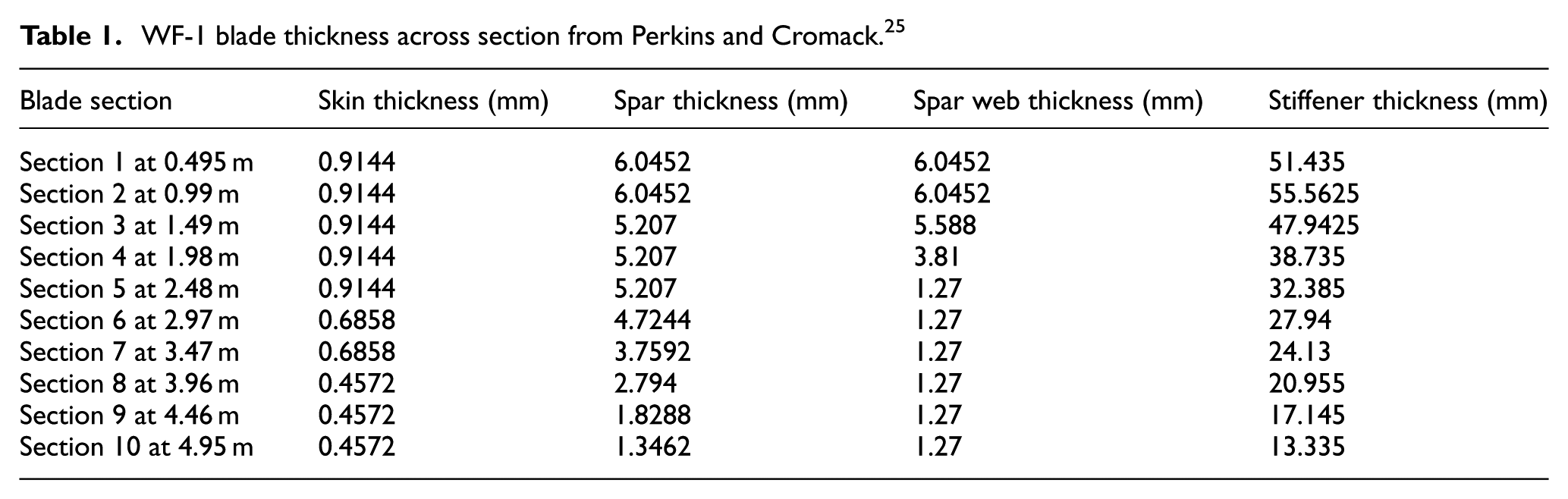
The blade section and planform are defined in Figures 2 and 3. The blade geometry details are shown in Tables 1 and 2, and material properties of blade parts are shown in Table 3.

Figure 2.

A sample blade section at 0.495 m from root as defined by Perkins and Cromack.²⁵

Figure 3.

Blade Planform as defined by Perkins and Cromack.²⁵

Table 1.

WF-1 blade thickness across section from Perkins and Cromack.²⁵

Blade section	Skin thickness (mm)	Spar thickness (mm)	Spar web thickness (mm)	Stiffener thickness (mm)
Section 1 at 0.495 m	0.9144	6.0452	6.0452	51.435
Section 2 at 0.99 m	0.9144	6.0452	6.0452	55.5625
Section 3 at 1.49 m	0.9144	5.207	5.588	47.9425
Section 4 at 1.98 m	0.9144	5.207	3.81	38.735
Section 5 at 2.48 m	0.9144	5.207	1.27	32.385
Section 6 at 2.97 m	0.6858	4.7244	1.27	27.94
Section 7 at 3.47 m	0.6858	3.7592	1.27	24.13
Section 8 at 3.96 m	0.4572	2.794	1.27	20.955
Section 9 at 4.46 m	0.4572	1.8288	1.27	17.145
Section 10 at 4.95 m	0.4572	1.3462	1.27	13.335

Table 2.

WF-1 blade specifications from Perkins and Cromack.²⁵

Blade length	16.25 ft (4.95 m)
Section profile	NACA4415
Maximum chord length	1.35 ft (0.411 m)
Minimum chord length	0.35 ft (0.107 m)
Maximum blade twist	45° near root

Table 3.

WF-1 blade material characteristics from Perkins and Cromack.²⁵

Component	Material	Moduli (GPa)	Density (kg/m³)
Skin	Low-modulus fiberglass epoxy	$\begin{matrix} E_{s k i n} = 15.168 \\ G_{s k i n} = 3.447 \end{matrix}$	2000
Spar, web, and stiffener	High-modulus fiberglass epoxy	$\begin{matrix} E_{s p a r} = 30.336 \\ G_{s p a r} = 2.068 \end{matrix}$	1500
Stock	Fiberglass epoxy with steel sleeve	E = 200	7850

The blade is made up of four parts: skin, spar, spar web, and stock. The skin composition is of fiberglass epoxy matrix having low bending modulus. The spar and the web are made of high-modulus fiberglass epoxy matrix and the stock is surrounded by a steel sleeve. The purpose of spar and spar web is to provide reinforcements to the hollow interiors of the blade. A trailing-edge stiffener is provided to prevent the top and bottom faces from attaching to each other near the trailing edge in case of heavy loads.

In order to maintain the aerodynamic configuration as per the specification, a high-fidelity 3D CAD model of the blade airfoil section and the blade is created using CATIA V5 3D modeling software. The airfoil sections are drawn as per the chord lengths and span locations defined in Figure 1 and the twists were applied to them as specified. The airfoil sections were connected by spline curves and a surface model is created. Figure 4 shows the airfoil sections and assembly of the blade CAD model.

Figure 4.

Details of blade model: (a) NACA 4415 profile for cross section, (b) blade surface, (c) wireframe, and (d) blade spar, web, and stiffener.

Blade structural analysis

FEM of the blade

The blade assembly is composed of four parts, which are the handle, skin, stiffener, and the shear web. These parts are assigned the thicknesses and material properties as defined in Table 2 and Figure 2, respectively. The FE model of the blade was created using the ANSYS software. The mesh was created using 71,212 elements and 141,385 nodes in the model. The root of the blade handle was fixed for all degrees of freedom (DOF) to create a fixed boundary condition for cantilever to simulate the root joint with turbine hub. Figure 5(a) and (b) shows blade’s 3D CAD and meshed model, respectively.

Figure 5.

Blade model: (a) CAD model and (b) FE model.

Natural frequency analysis

In order to validate the correctness of the developed simulation model of the blade, the natural frequencies of the blade are calculated and compared with the reference solution by Perkins and Cromack.²⁵ The block Lanczos method is used to perform the modal analysis as it is widely used. The vibration modes of first three orders were extracted. Figure 6 shows the three modes and Table 4 shows the observed natural frequencies and comparison with the reference (experimental and numerical predictions). As shown in Figure 6 and Table 4, the most important top three modes of the developed blade match well with the reference blade.

Figure 6.

Natural frequency and mode shapes: (a) mode I, (b) mode II, and (c) mode III.

Table 4.

Blade natural frequencies.

Mode	Mode	Natural frequency	From Perkins and Cromack²⁵
		Observed	Measured	Numerical prediction
1	Flapwise	31.57 rad/s (5.03 Hz)	25 rad/s (3.98 Hz)	28 rad/s (4.46 Hz)
2	Edgewise	61.01 rad/s (9.71 Hz)	56 rad/s (8.91 Hz)	65 rad/s (10.35 Hz)
3	Flapwise	93.43 rad/s (14.87 Hz)	84 rad/s (13.37 Hz)	93 rad/s (14.80 Hz)

The difference between the observed natural frequencies with the reference numerical prediction can be attributed to uncertainty in the available geometry details such as trailing-edge region, stiffener thickness, and resin-steel sleeve at the handle. This uncertainty could have resulted in lesser flexibility in the model especially for the second mode. However, since flapwise bending is more critical for fatigue load,¹⁰ the variation in edgewise mode can be accepted.

Static structural analysis

The blade is subjected to static loads to check whether the deflection and bending stresses on top and bottom surfaces are computed correctly as compared with reference solution by Perkins and Cromack.²⁵ The load applied is 68.95 N acting downward with blade in horizontal position (15 lbs and 8 Oz as per reference) at a location of 0.95R where R is the blade span radius. The results for the deflection of the free end and the maximum bending stresses on top and bottom surfaces at a section located at 0.475R along with comparison with reference is shown in Table 5. Figures 7 and 8 show these simulation results from ANSYS computer-aided engineering (CAE) software.

Table 5.

Blade deflections and maximum bending stress under applied reference load.

		Current blade	Reference blade²⁵
Tip deflection (mm)	U (vertical)	13.69	14.5
	V (horizontal	72.3	76
Maximum bending stress (MPa)	Top surface (compression)	−3.73	−3.88
	Bottom surface (tensile)	+3.26	+3.21

Figure 7.

Deflections of blade free end: (a) vertical deflection and (b) horizontal deflection.

Figure 8.

Bending stresses on (a) top and (b) bottom surfaces at 0.475R.

The variation in the bending stress on the top (suction) and bottom (pressure) surfaces of the blade across the chord length was found out at a specified location of 0.475R in the reference. Figure 9 shows a good agreement between the observed and the reference distribution.

Figure 9.

Comparison of observed and reference Perkins and Cromack²⁵ bending stresses on top and bottom surfaces of the blade at a location of 0.475R.

Thus, the baseline model of the blade is established having structural response close to the reference. This blade model is further analyzed for transient and fatigue analysis in next section.

Wind field modeling and forecasting

For the Salem location, the information available for the mean wind speed and Weibull parameters for wind distribution for each month of the year is referred from the works of Sriram et al.³⁵ The parameters are based on the data taken every 4 h on Monday, Wednesday, and Friday during 2001 and 2002 time period. The Weibull distribution function is defined as

f (V) = \frac{K}{C} {(\frac{V}{C})}^{k - 1} {〖 \exp 〗}^{{[- V / C]}^{k}}

(1)

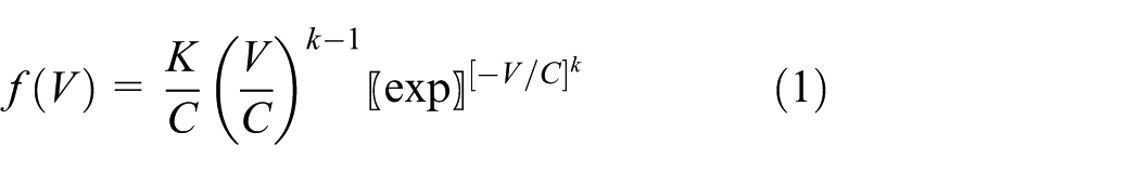
where K and C are shape and scale parameters, respectively, and V is the wind speed. These parameters for each month of the above-mentioned period are given in Table 6.

Table 6.

Average monthly wind speed and Weibull parameters.

S. no.	Month	From Sriram et al.³⁵
		Average wind velocity (m/s)	Shape parameter (K)	Scale parameter (C)
1	April 2001	2.95	5.0467	3.2495
2	May	3.51	4.9083	3.7978
3	June	2.91	6.2790	3.2195
4	July	1.94	4.0466	2.6134
5	August	1.41	3.0215	1.5671
6	September	1.38	3.4941	1.5474
7	October	1.12	4.5830	1.2318
8	November	1.30	3.0281	1.4714
9	December	1.90	8.9593	2.0786
10	January 2002	2.25	5.8633	2.3088
11	February 2002	2.46	7.7020	2.6013
12	March 2002	1.98	4.6899	2.1418

As mentioned in section “Introduction,” the details of the three stochastic forecasting models—first-order Markov chain, ARIMA, and Kalman filter—and their comparison for the wind prediction are discussed in the following.

Markov chain

This is a discrete time model made of sequence of random variables $X_{1}, X_{2}, X_{3}, \dots$ such that the future state $X_{n + 1}$ is not dependant on the past states $X_{n - 1}, X_{n - 2}, \dots$ but only on the present state $X_{n}$

\begin{matrix} P_{r} (X_{n + 1} = x_{n + 1} | X_{1} = x_{1}, X_{2} = x_{2}, \dots, X_{n} = x_{n}) \\ = P_{r} (X_{n + 1} = x_{n + 1} | X_{n} = x_{n}) \end{matrix}

(2)

The set of possible states of $X_{n} S = {s_{1}, s_{2}, s_{3}, \dots, s_{k}}$ are called state space of the chain and the probability of the chain to move from state $s_{i} to s_{j}$ , that is, $p_{i j}$ is called as transition probability from state i to j with $s_{1} \leq s_{i}, s_{j} \leq s_{k}$

p_{i j} = P_{r} (X_{1} = s_{j} | X_{0} = s_{i})

(3)

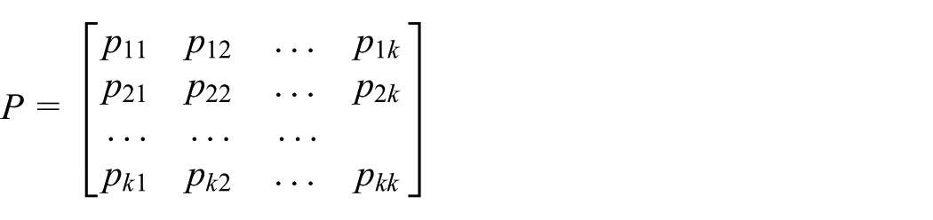
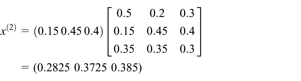
The probability distribution of transitions from one state to another can be represented into a transition matrix $P = (p_{i j})_{i, j}$ . For K state, the first-order transition probability matrix P has a size of K × K and has the form

P = [\begin{matrix} p_{11} & p_{12} & \dots & p_{1 k} \\ p_{21} & p_{22} & \dots & p_{2 k} \\ \dots & \dots & \dots \\ p_{k 1} & p_{k 2} & \dots & p_{k k} \end{matrix}]

So, for a three-state chain, it can be represented as

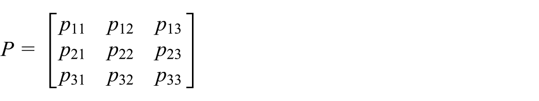
P = [\begin{matrix} p_{11} & p_{12} & p_{13} \\ p_{21} & p_{22} & p_{23} \\ p_{31} & p_{32} & p_{33} \end{matrix}]

or let us say with an example

P = [\begin{matrix} 0.5 & 0.2 & 0.3 \\ 0.15 & 0.45 & 0.4 \\ 0.25 & 0.35 & 0.4 \end{matrix}]

This means that p₁₂ = 0.2 is the probability of system to go from state 1 to state 2, that is, $X_{1} = s_{2}$ if it is currently at $X_{0} = s_{1}$ . Similarly, the probability distribution of states after first step and second step if it currently in state $X_{0} = s_{1}$ is

x^{(1)} = (010) [\begin{matrix} 0.5 & 0.2 & 0.3 \\ 0.15 & 0.45 & 0.4 \\ 0.35 & 0.35 & 0.3 \end{matrix}] = (0.15 0.45 0.4)

\begin{matrix} x^{(2)} = (0.15 0.45 0.4) [\begin{matrix} 0.5 & 0.2 & 0.3 \\ 0.15 & 0.45 & 0.4 \\ 0.35 & 0.35 & 0.3 \end{matrix}] \\ = (0.2825 0.3725 0.385) \end{matrix}

If all the states in the matrix communicate, that is, $s_{i} \to s_{j}$ and $s_{j} \to s_{i}$ (both states can be accessible from each other with positive probability), then the matrix P is said to be irreducible.

The availability of Weibull parameters and mean wind speed for each month of the year as shown in Table 6 accounts for the seasonality of the wind. For each month of the year, the wind speed vectors are generated based on the mean wind speed (Table 6) and maximum wind speed for Salem which falls in zone 4.³⁶ These data are used to create a Weibull probability density for the vector values. The transition parobability matrix for each month is then defined using the procedure for simulating non-Gaussian wind speed time series.³⁷ This matrix relates each hourly wind speed value with previous hourly average based upon (1) desired probability density as per monthly Weibull parameters and (2) autocorrelation of wind speed. Hence, the transition matrix is modeled as a normalized product of a diagonal probability matrix for probability density and a suitable symmetric decay matrix for autocorrelation.

Validation of Markov approach with a reference wind measurement

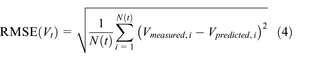
The above method is first validated against a measured wind data,^38,39 and the comparison for the predicted and the measured wind is shown in Table 7 in terms of root mean square error (RMSE), MAE error metrics, and the Weibull parameters. The measured wind data considered here are for the Iowa, USA location every 10 min from 1 January 2008 till 31 December 2008. There are 52,704 observations and the wind speed range is from 0.35 to 19.22 m/s. The RMSE is defined as

RMSE (V_{t}) = \sqrt{\frac{1}{N (t)} \sum_{i = 1}^{N (t)} {(V_{m e a s u r e d, i} - V_{p r e d i c t e d, i})}^{2}}

(4)

Table 7.

RMSE, MAE, and Weibull parameter comparison of Markov prediction with measured wind.

	RMSE	MAE	Measured wind		Predicted wind
			Weibull shape (K)	Weibull scale (C)	Weibull shape (K)	Weibull scale (C)
March 2008	2.0076	0.61	9.141	2.229	9.194	2.278
July 2008	0.9949	0.50	8.03	2.062	8.107	2.083
November 2008	1.1658	0.79	10.489	2.279	10.419	2.24

The benefit of using RMSE as metric for comparison is that it brings in more weightage on larger error terms due to the square of the difference term.

Another commonly used error metric called MAE is calculated. MAE is defined as

MAE (V_{t}) = \frac{1}{N (t)} \sum_{i = 1}^{N (t)} | V_{m e a s u r e d, i} - V_{p r e d i c t e d, i} |

(5)

where $V_{m e a s u r e d, i}$ and $V_{p r e d i c t e d, i}$ are the measured and predicted wind speed at ith time instant and N(t) is the total number of observations (Figure 10). These RMSE and MAE error ranges match with other published results such as Zastrau et al.⁴⁰

Figure 10.

Comparison of observed and predicted wind for the month of March 2008.

Application of Markov method for Salem location

The Markov method which is tested with reference wind is now applied for the Salem city in India having the Weibull parameters and mean wind speed as defined in Table 6. The approach of including seasonality for long-term wind prediction where the actual measurements are limited is also used by researchers like Karatepe and Corscadden⁴¹ with good results. The wind prediction using Markov and Kalman methods for months having maximum and minimum of mean wind speed is shown in Figure 11. Figure 12 shows the predicted wind speed for Salem for 1 year and its PDF is calculated using MATLAB.

Figure 11.

Hourly wind prediction based on Markov chain and Kalman filter for Salem city for (a) May and (b) October months of the year which have maximum and minimum mean wind speed, respectively.

Figure 12.

(a) Wind speed for 1 year generated by Markov chain and (b) Weibull probability distribution.

The transition probability matrix from Markov approach is shown in Tables 8 and 9 for November and April months, respectively, which have minimum and maximum mean speeds, respectively. This matrix is based on 12 bins for wind speed ranging from 0 to 12 m/s with 1 m/s interval.

Table 8.

Markov probability transition matrix for November having mean wind speed of 1.3 m/s.

	1	2	3	4	5	6	7	8	9	10	11	12
1	0.758	0.200	0.036	0.005	0.001	0.000	0.000	0.000	0.000	0.000	0.000	0.000
2	0.080	0.762	0.135	0.020	0.003	0.000	0.000	0.000	0.000	0.000	0.000	0.000
3	0.012	0.116	0.744	0.111	0.015	0.002	0.000	0.000	0.000	0.000	0.000	0.000
4	0.002	0.021	0.136	0.732	0.096	0.011	0.001	0.000	0.000	0.000	0.000	0.000
5	0.000	0.004	0.029	0.153	0.720	0.084	0.009	0.001	0.000	0.000	0.000	0.000
6	0.000	0.001	0.007	0.036	0.169	0.706	0.074	0.007	0.000	0.000	0.000	0.000
7	0.000	0.000	0.002	0.009	0.044	0.184	0.690	0.065	0.000	0.000	0.000	0.000
8	0.000	0.000	0.001	0.003	0.013	0.053	0.199	0.671	0.057	0.004	0.000	0.000
9	0.000	0.000	0.000	0.001	0.004	0.017	0.063	0.214	0.653	0.046	0.002	0.000
10	0.000	0.000	0.000	0.000	0.002	0.006	0.024	0.080	0.244	0.616	0.028	0.001
11	0.000	0.000	0.000	0.000	0.001	0.003	0.012	0.040	0.121	0.307	0.501	0.015
12	0.000	0.000	0.000	0.000	0.000	0.002	0.008	0.026	0.081	0.204	0.332	0.347

Bold value shows the probability of wind speed staying in same bin/range.

Table 9.

Markov probability transition matrix for April having mean wind speed of 2.95 m/s.

	1	2	3	4	5	6	7	8	9	10	11	12
1	0.714	0.227	0.048	0.009	0.001	0.000	0.000	0.000	0.000	0.000	0.000	0.000
2	0.091	0.723	0.154	0.027	0.004	0.001	0.000	0.000	0.000	0.000	0.000	0.000
3	0.017	0.132	0.703	0.126	0.020	0.003	0.000	0.000	0.000	0.000	0.000	0.000
4	0.004	0.029	0.154	0.688	0.108	0.015	0.002	0.000	0.000	0.000	0.000	0.000
5	0.001	0.007	0.039	0.172	0.674	0.094	0.012	0.001	0.000	0.000	0.000	0.000
6	0.000	0.002	0.011	0.048	0.189	0.657	0.082	0.009	0.001	0.000	0.000	0.000
7	0.000	0.001	0.003	0.015	0.059	0.205	0.638	0.072	0.007	0.000	0.000	0.000
8	0.000	0.000	0.001	0.005	0.020	0.070	0.219	0.615	0.062	0.005	0.000	0.000
9	0.000	0.000	0.000	0.002	0.008	0.027	0.083	0.234	0.593	0.050	0.003	0.000
10	0.000	0.000	0.000	0.001	0.003	0.012	0.037	0.103	0.262	0.550	0.030	0.001
11	0.000	0.000	0.000	0.000	0.002	0.007	0.021	0.059	0.150	0.315	0.430	0.015
12	0.000	0.000	0.000	0.000	0.001	0.005	0.016	0.044	0.110	0.231	0.315	0.277

Bold value shows the probability of wind speed staying in same bin/range.

ARIMA model

ARIMA is a type of statistical method for time series–based forecasting which combines the “autoregression” (AR), that is, modeling the linear dependence of the output on its past “p” values, and “moving average” (MA), that is, the linear dependence of the error/residual term on the current and past “q” values of stochastic error terms. ARIMA is a special case of the ARMA model where the non-stationary time series is differentiated “d” times to make it stationary. Thus, the general equation for ARIMA (p,d,q) model for a variable Y is constructed as follows.

If Y is the dth differential of Y such that

y_{t} = Y_{t} when d = 0

(6a)

y_{t} = Y_{t} - Y_{t - 1} for d = 1

(6b)

\begin{matrix} y_{t} = (Y_{t} - Y_{t - 1}) - (Y_{t - 1} - Y_{t - 2}) \\ = (Y_{t} - Y_{t - 1} + Y_{t - 2}) for d = 2 \end{matrix}

(6c)

\begin{matrix} y_{t} = φ_{1} y_{t - 1} + \dots + φ_{p} y_{t - p} + \in_{t} \\ + {θ_{1}}_{t - 1} + \dots + {θ_{q}}_{t - q} \end{matrix}

(7a)

y_{t} = \in_{t} + \sum_{i = 1}^{p} φ_{i} y_{t - i} + \sum_{i = 1}^{q} {θ_{i}}_{t - i} \in_{t - 1}

(7b)

where $φ_{i}$ and $θ_{i}$ are the autoregressive and MA parameters, respectively, to be determined. $\in_{t}$ are the error terms (white noise) with normal distribution and zero mean.

The process to generate the forecast data is to first estimate p, q, and d by differencing the data and iteratively checking autocorrelation function (ACF) plots for q and partial autocorrelation function (PACF) plots for p till stationary trend is obtained. Thus, the value of p is determined as the last lag after which the PAC cuts off and the value of q is determined from the last lag after which ACF cuts off. 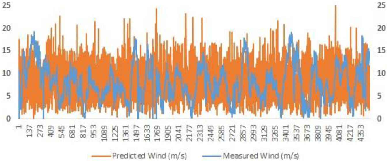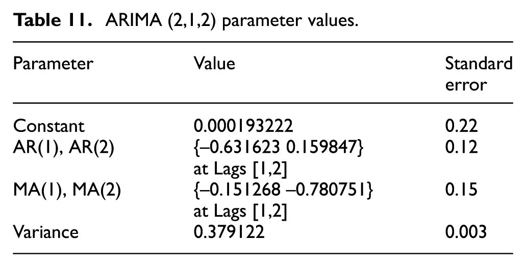This identification phase is followed by finding $φ_{i}$ and $θ_{i}$ parameters using maximum likelihood estimation (MLE) techniques or backcasting methods which is the estimation phase. Once the model is fit, diagnostic checks are done on autocorrelation plots of the residuals to see whether any large autocorrelation exist. The values of p and q are adjusted if needed. This is the final diagnostic check phase.

For wind prediction using ARIMA model, the wind generated using Markov Chain is used as training data. A software program is developed in MATLAB to find the autocorrelation and partial autocorrelation plots of the wind. Using the MATLAB functions “estimate,” the AR, MA, and integration parameters are found to be of ARIMA (2,1,2) series which has lowest Akaike information criterion (AIC) and Bayesian information criterion (BIC) values as seen from Table 10 when compared to some of the other trials. The AIC and BIC criteria are a standard criteria for ARIMA-based model selection.⁴² The parameters of the ARIMA (2,1,2) model are given in Table 11 showing the goodness of the fit. The ARIMA prediction 1 month ahead wind speed is shown in Figure 13, and Figure 14 shows the ACF and PACF plots of the training input.

Table 10.

ARIMA models’ comparison.

	ARIMA (2,1,2)	ARIMA (1,1,2)	ARIMA (2,1,1)	ARIMA (3,1,3)	ARIMA (1,1,1)
AIC	−4232.32	−4223.21	−4223.442	−4228.105	−4219.627
BIC	−4192.12	−4194.96	−4195.185	−4198.778	−4203.129

Table 11.

ARIMA (2,1,2) parameter values.

Parameter	Value	Standard error
Constant	0.000193222	0.22
AR(1), AR(2)	{–0.631623 0.159847} at Lags [1,2]	0.12
MA(1), MA(2)	{−0.151268 −0.780751} at Lags [1,2]	0.15
Variance	0.379122	0.003

Figure 13.

Markov chain wind pattern and 1 month ahead ARIMA prediction.

Figure 14.

Autocorrelation and partial autocorrelation plots for the Markov wind data.

Kalman filter

In this model, the unknown state vector $X_{t}$ is defined over a range of time steps t as follows

X_{t + 1 / t} = A_{t / t} \times X_{t / t} + w_{t}

(8)

And the correlation between measured vector and unknown state vector is defined as

Z_{t + 1 / t} = C_{t / t} \times_{t + 1 / t} + v_{t}

(9)

where $A_{t}, C_{t}$ are the matrices in the state-space equation; $X_{t / t}, X_{t + 1 / t}$ are the state of the system; $Z_{t + 1 / t}$ is the output prediction from Kalman filter; and $w_{t}, v_{t}$ is the system and measurement noise, respectively.

The wind spectrum based on Kalman filter proposed by Kalman⁴³ is expressed as

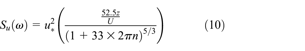
S_{u} (ω) = u_{*}^{2} (\frac{\frac{52.5 z}{U}}{{(1 + 33 \times 2 π n)}^{5 / 3}})

(10)

where U is the mean wind speed, z is the height above ground, $u_{*}$ is the friction velocity, $n = f z / U [f = (f_{s} / N) * (1 : N / 2)]$ , $f_{s}$ is the sampling frequency, and N is the total number of points.

The standard deviation ( $σ_{X_{t}}^{2}$ ) for each Fourier coefficient $X_{t} = (T / 2 π) S_{u} (ω)$ . The Fourier coefficients for above spectrum are generated using complex numbers to represent time series in real numbers. For this, a vector of Fourier coefficients $C_{n}$ of length N of N/2 coefficients $a_{n}$ and $b_{n}$ are generated such that

\begin{matrix} (C_{n})_{0 \dots N - 1} = [\frac{T U}{2 π}]; \\ a_{1} + i b_{1}; \dots; a_{\frac{N}{2} - 1} + i b_{\frac{N}{2} - 1}; + a_{\frac{N}{2} - 1} + 0; \\ a_{\frac{N}{2} - 1} - i b_{\frac{N}{2} - 1}; \dots; a_{1} - i b_{1} \end{matrix}

(11)

and the standard deviation is distributed equally among the real and imaginary parts, that is

σ_{a_{n}}^{2} = σ_{b_{n}}^{2} = \frac{1}{2} σ_{x_{n}}^{2}

(12)

Then, inverse Fourier transform is applied on the generated Fourier coefficients to get the series values in the time domain

X_{m} = 2 π \frac{f_{s}}{N} i f f t

(13)

Thus, looking at the accuracy of the Markov method to predict wind speed based on monthly Weibull wind speed characteristics (section “Validation of Markov approach with a reference wind measurement”) and the higher alternating wind speed prediction compared to Kalman and almost constant mean speed prediction by ARIMA model, Markov chain model is selected for wind speed forecast and blade fatigue load calculation.

Aerodynamic wind load calculation

The wind prediction obtained for 1 year using Markov chain method from previous section is used to calculate the aerodynamic forces on the blade section using the BEM method. A software program is developed in MATLAB which utilizes the varying wind speeds from Markov prediction and the flowchart in Figure 15 for calculating the hourly time-varying thrust and moment loads for the 10 blade sections for all the months of the year. Blade rotational speed is taken as 12 r/min. Thus, a duty cycle for 1 year is created. Figure 16 shows the loads and moments on some sections (1, 2, 5, 6, 9 and 10) for 1 month duration.

Figure 15.

Flowchart for calculating induction factors and blade forces and moments.

Figure 16.

Loads and moments on some blade sections for 1 month.

Comparison of static load calculation by BEM method with analytical method

The major loads on the wind turbine blade are due to wind itself along with gravitational force in horizontal position. The centrifugal forces are comparatively low due to low rotational speed. The lift and drag forces on the blade as given by Yahya⁴⁴ are

F_{L i f t} = \frac{1}{2} ρ V^{2} A C_{L}

(14)

F_{D r a g} = \frac{1}{2} ρ V^{2} A C_{D}

(15)

where $ρ$ is the density of air (1.225 kg/m³), V is the mean wind velocity which is taken as 10 m/s, A is the swept area of blade, and $C_{L} C_{D}$ are the lift and drag coefficients (0.86 and 0.0126, respectively) for the airfoil considering angle of attack at 4.1° and a Reynolds number of 1 million as referred from Hoffman et al.⁴⁵ which is shown in Figure 17.

Figure 17.

Lift and drag coefficients for NACA4415⁴⁵ at Re = 1E6.

The gravity force $F_{g} = m g$ , where m is the blade mass and the $F_{r} = m R ω^{2}$ , where R is the blade span radius and $ω$ is the angular speed of rotor. Table 12 shows the important parameters for dynamic loads on the current blade and Figure 18 shows the lift and drag forces on blade.

Table 12.

Parameters for dynamic loading.

R, L (blade span)	4.953 m
$ω$ (angular speed)	1.257 rad/s
m (blade mass)	24 kg

Figure 18.

Aerodynamic forces on blade.⁴⁶

Thus, the BEM-based program calculation for static structural loads matches the analytical solution with acceptable tolerance as seen from Table 13. The resultant thrust loads closely match. Many authors such as D Salimi-Majd et al.⁴⁷ have used this approach to find approximate blade loads.

Table 13.

Static load comparison of BEM and analytical approaches.

	By BEM-based program (N)	By analytical method^44,46 (N)
Lift force	1784.66	1841
Drag force	314.68	41
Total thrust	1812.2	1841.5

BEM: blade element momentum.

Blade fatigue analysis

The time-varying wind loads and moments on blade calculated in section “Aerodynamic wind load calculation” are used as basis for the fatigue analysis. The load cycle is made of 1 year of loads with data point for each hour of a month for the selected site of Salem. Thus, there are 8760 load points in the cycle. In order to create the time-varying signal, first static analysis is carried out by taking the peak values of load and moment. Then, a non-dimensional signal is created by dividing actual loads by the peak loads used in the static analysis. The equivalent von Mises stress obtained from static analysis is used as a basis for fatigue analysis. Figure 19(a) shows the applied loads in static analysis and Figure 19(b) shows the Von Mises stress distribution.

Figure 19.

(a) Loading, (b) equivalent von Mises stress, and (c) maximum principal stress for static analysis.

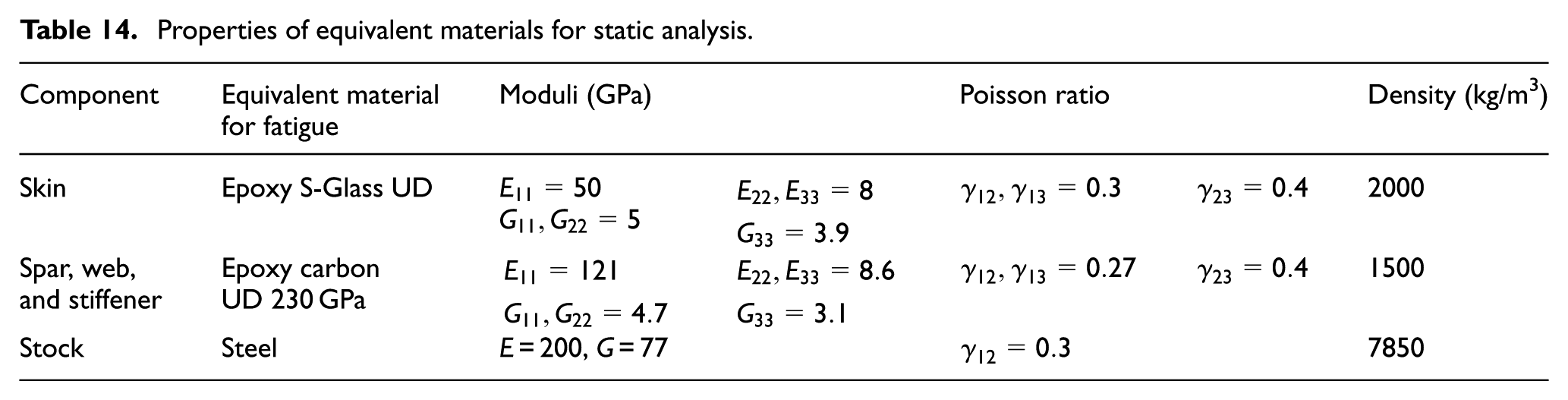
Since the reference material by Perkins and Cromack²⁵ does not contain enough information for fatigue analysis, equivalent materials for skin, spar, web, and stiffener are chosen as shown in Table 14 for carrying out static analysis as first step. The material properties for these materials are obtained from SNL/MSU/DOE Composite Material Fatigue Database.⁴⁸

Table 14.

Properties of equivalent materials for static analysis.

Component	Equivalent material for fatigue	Moduli (GPa)		Poisson ratio		Density (kg/m³)
Skin	Epoxy S-Glass UD	$E_{11} = 50$ $G_{11}, G_{22} = 5$	$\begin{matrix} E_{22}, E_{33} = 8 \\ G_{33} = 3.9 \end{matrix}$	$γ_{12}, γ_{13} = 0.3$	$γ_{23} = 0.4$	2000
Spar, web, and stiffener	Epoxy carbon UD 230 GPa	$\begin{matrix} E_{11} = 121 \\ G_{11}, G_{22} = 4.7 \end{matrix}$	$\begin{matrix} E_{22}, E_{33} = 8.6 \\ G_{33} = 3.1 \end{matrix}$	$γ_{12}, γ_{13} = 0.27$	$γ_{23} = 0.4$	1500
Stock	Steel	E = 200, G = 77		$γ_{12} = 0.3$		7850

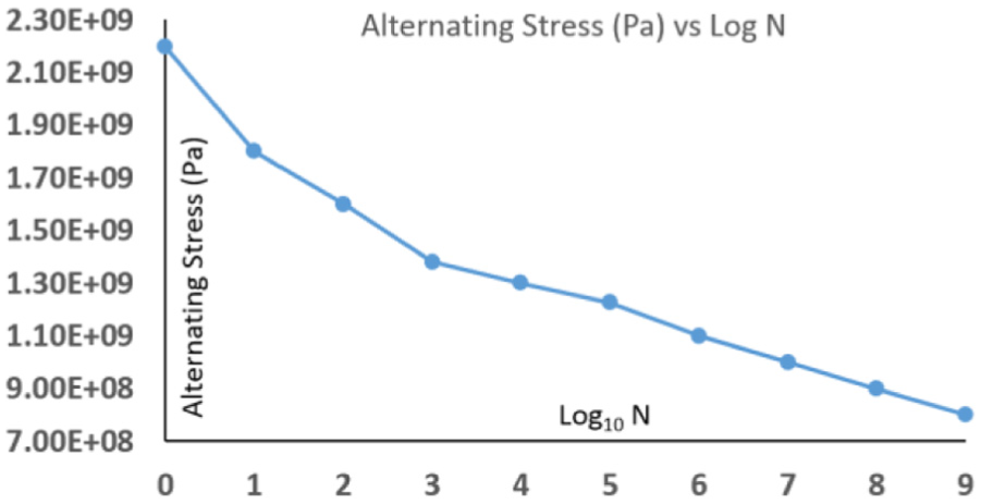
The S-N curves for skin and spar, web, and stiffener materials are shown in Figures 20 and 21, respectively, which are used for fatigue analysis. These S-N curves are generated from the constant life diagrams (CLDs) referred from Mandell et al.⁴⁹

Figure 20.

S-N curve for skin material at stress ratio R = –1 (Epoxy S-Glass UD).

Figure 21.

S-N curve for spar, web and stiffener material at stress ratio R = –1 (Epoxy Carbon UD 230 GPa).

After performing the static analysis, the time-varying load signal is used to calculate the fatigue life, damage, and safety factor for the blade. The stress life approach is used with Goodman’s criteria for mean stress correction and von Mises stresses are used as stress component. It is seen that the blade has the available life of around 28 years and corresponding damage of 3.58 for the load cycle shown in Figure 16. The load scale factor is then varied to see the effect on fatigue. Figure 22 shows the variation of available life (years), accumulated damage, and safety factor at the fatigue critical location (FCL) with the load scaling from 0.25 to 2.5. Figure 23(a)–(d) shows the available life, factor of safety, damage, and the rainflow cycle plots, respectively, at the FCL which is on the skin near the root of the blade. These plots are for a 1-year load cycle made of 8760-h signal. The life units are in hours and stress ratio R is −1. The design life is taken as 40 years (350 and 400 h).

Figure 22.

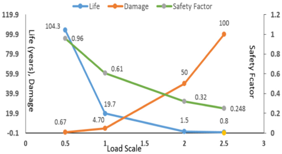
Variation in available life, damage, and safety factor with load scaling at stress ratio R = –1 and S-Glass as skin material.

Figure 23.

(a) Available life in FCL zone (2.443E05 h = 27.9 Years), (b) safety factor in FCL zone, (c) damage in FCL zone, and (d) rainflow amplitudes and mean values for stress ratio R = –1 and von Mises criteria.

Effect of stress ratio

The importance of studying the effect of stress ratio R on the fatigue life of composite materials was highlighted by authors such as Huh et al.⁵⁰ and Roundi et al.⁵¹ Most of the studies have focused either on tension–tension or compression-only loadings. Gambone,⁵² however, has analyzed a wide range of stress ratios −1 ≤ R ≤ 0.5 and its effect on the mode-II delamination of carbon/epoxy composites in terms of strain energy release rate range $(Δ G_{I I})$ , maximum strain energy release rate $(G_{I I m a x})$ , and stress intensity factor range $(Δ K_{I I})$ . He concluded that increase in R ratio leads to decrease in crack growth rate (da/dN) over a given $Δ G_{I I}$ as well as when evaluated as a function of $G_{I I m a x}$ .

Hence, present authors have carried out fatigue analysis of the blade for stress ratios of −1, −0.5, 0.1, and 0.5, and the results are shown in Figure 24. It shows the effect of stress ratio on the fatigue parameters. It is seen that the stress ratio for fully reversed condition of −1 is the least favorable while with R = 0.5 is the most favorable. These findings are in line with the similar studies mentioned above and can be explained by the fact that stress ratio of −1 means a high stress amplitude as compared to positive ratio.

Figure 24.

Variation in available life, damage, and safety factor with stress ratio (R) and S-Glass as skin material.

The von Mises stress variation at the node where maximum static stress is found is calculated from the load signal and the static analysis results. A software program in MATLAB is created to extract the rainflow cycles from the variable nodal stresses. The rainflow matrix in Figure 23(d) shows that the smaller stress amplitudes up to 4 MPa are more in number and contribute more to the fatigue failure than the large stress amplitudes. Note that due to some modeling error far away from root zone, there are some areas where high damage and low life are shown by the ANSYS tool which can be ignored as it is not in the FCL zone near the blade root.

Effect of stress criteria

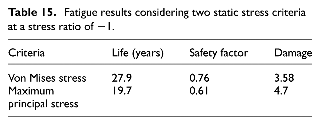
The fatigue analysis is also carried out by considering the maximum principal stress criteria. Table 15 shows the difference in the fatigue life and safety factor for maximum principal stress and von Mises stress criteria and Figure 25 shows these plots. It is seen that the maximum principal stress accounts for lower fatigue life and safety factor than von Mises criteria due to higher principal stresses as seen in other studies.⁵³

Table 15.

Fatigue results considering two static stress criteria at a stress ratio of −1.

Criteria	Life (years)	Safety factor	Damage
Von Mises stress	27.9	0.76	3.58
Maximum principal stress	19.7	0.61	4.7

Figure 25.

(a) Available life in FCL zone (1.72E5 h = 19.7 years) and (b) safety factor in FCL zone for stress ratio R = –1 and maximum principal stress criteria.

Analysis with different skin materials

The fatigue life, damage, and factor of safety were also calculated by doing analysis with glass fiber–reinforced epoxy laminate (QQ1) and carbon/glass-hybrid-fiber-reinforced epoxy (P2B) for skin material. The material properties are shown in Table 16 which are first used to do static analysis.

Table 16.

Material properties for various skin materials.

Property	Epoxy S-Glass UD⁵⁴	QQ1 (E-Glass UD)⁴⁹	P2B (Carbon/Glass-hybrid Epoxy)⁴⁹
E11	56 GPa	33.1 GPa	101 GPa
$γ_{12}$	0.3	0.27
$γ_{13}, γ_{22}$	0.4	0.44
E22, E33	11.4 GPa	11.93 GPa	13.7 GPa
G12	4.48 GPa	4.33 GPa	4.33 GPa
Ultimate strength (tensile)	1.98 GPa	0.843 GPa	1.546 GPa
Ultimate strength (compression)	0.626 GPa	0.687 GPa	1.047 GPa
Tensile yield strength	0.2 GPa	0.149 GPa	0.08 GPa
Compressive yield strength	0.4 GPa	0.274 GPa	0.24 GPa
Density	1800 kg/m³	1919 kg/m³	1570 kg/m³

QQ1 is the glass-fiber-reinforced epoxy laminate made up of Vantico TDT 177-155 Epoxy Resin, Saertex U14EU920-00940-T1300-100000 0’s, and VU-90079-00830-01270-000000 45’s fabrics. P2B is a carbon/glass-hybrid-fiber-reinforced epoxy laminate made up of Newport carbon NB307-D1-34-600 G300 prepreg at 0° and glass NB307-D1-7781-497A at ±45°. The S-N curves for QQ1 and P2B were calculated using the CLD referred from Mandell et al.⁴⁹ and shown in Figure 26. The S-N curves are shown in Figure 27(b) and (c). These properties are used for the fatigue analysis. The fatigue results for various load scales are shown in Figure 28 for all the three skin materials.

Figure 26.

Constant life diagrams (CLDs) for carbon and glass fibers for different stress ratios.⁴⁹

Figure 27.

S-N curve for skin materials: (b) QQ1 and (c) P2B for stress ratio R = –1.

Figure 28.

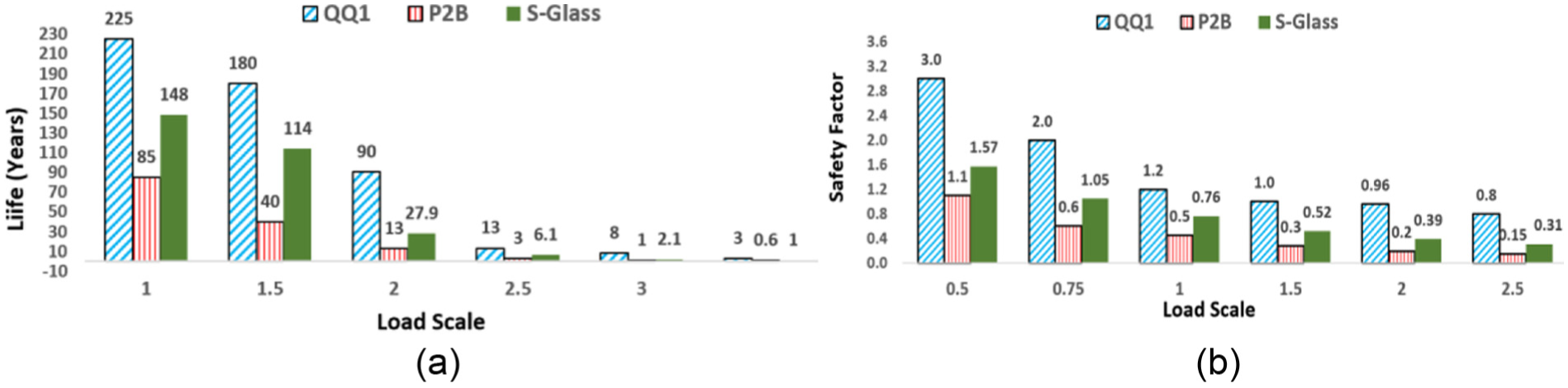
(a) Variation in fatigue life and (b) safety factor for different skin materials for stress ratio R = –1.

CZM of blade root joint

The root joint of the current blade consists of epoxy/resin composite core enclosed inside the steel sleeve. This adhesively bonded root joint is a critical area which can lead to delamination. The failure of the wind turbine root joint due to delamination has been studied by many researchers using CZM. The benefit of this method is the possibility of modeling debonding without requirement of crack and thus can be used to predict damage initiation in a healthy material.

Kalkhoran et al.⁵⁵ analyzed the debonding initiation and progression at the adhesive root joint of 23-m-long blade of a 660-kW HAWT using CZM approach. They implemented a cohesive zone constituent law based on dissipated energy and used double cantilever beam (DCB), end notch flexure (ENF), and mix mode bending (MMF) tests under static and fatigue loading for developing root joint material properties. The static analysis was effectively used to find the critical blade position for doing fatigue analysis.

Salimi-Majd et al.⁴⁷ analyzed the loading conditions at the root joint of a large wind turbine blade throughout a full rotation of the blade for the CZM-based fatigue analysis. They concluded that bending loads are more effective than the axial forces for failure of adhesively bonded root joint with blade horizontal position being critical due to high delamination index. This position and load ratio are taken as inputs for fatigue analysis. The load ratio R was defined as the ratio of minimum to maximum delamination index, while delamination index is a measure of relative strains at the beginning of delamination with those of the cohesive interface element.

Hosseini-Toudeshky et al.⁵⁶ analyzed the progressive fatigue debonding of the adhesively bonded root joint of a 660-kW wind turbine blade under cyclic loading using CZM modeling. They could verify the results of the numerical analysis for mode I, mode II, and mixed-mode crack initiation and propagation with experimental tests. They noted that the maximum length of the deboned area after a typical overloading can go up to 40% of the height of the root joint in 1 month of operation under fatigue loading and thus highlighted the significance of debonding analysis. Khoramishad et al.⁵⁷ developed a numerical damage model for adhesively bonded joints under fatigue loading that is only dependent on the adhesive system and not on joint configuration. They integrated a strain-based fatigue damage model with CZM model to simulate the damaging influence of the fatigue loading on the bonded joints. Bak et al.⁵⁸ developed a new method to simulate fatigue-driven delamination based on CZM which can predict both quasi-static and fatigue crack propagation. Their method directly links crack growth and damage evolution of cohesive zone to Paris law. This makes their method distinct with other available methods which have structural dependency on strain energy release rate. They also found good numerical convergence even at coarse meshes which is a significant benefit for computational efficiency to analyze complex turbine blades.

Considering the significance of the CZM-based damage analysis as seen from the above literature, the authors of this study carried out the CZM of the root joint with fatigue analysis to study its behavior under cyclic loads. The interface properties of the cohesive layer for mixed-mode loading are shown in Table 17. The static analysis is first carried out on the root joint modeled as cohesive zone. The results for the maximum principal stress and deflection are shown in Figure 29 which show the critical area in the interface zone.

Table 17.

Cohesive zone properties.

Property	Symbol	Value
Critical strain energy release rate, mode I	G_Ic	0.26 kJ/m²
Critical strain energy release rate, mode II	G_IIC	1.002 kJ/m²
Penalty stiffness	K	10E6 N/mm³
Interface strength in mode I and II	$T_{I}^{0}$ , $T_{I I}^{0}$	30 MPa
Benzeggagh–Kenane law parameter	η	2.73

Figure 29.

Maximum principal stress and deflection at the interlaminar region.

Fatigue analysis is then carried out by applying fully reversed load cycles for various load cycles. The results for the life and damage at the critical location found from fatigue analysis of the CZM model for various load cycles are shown in Figure 30. It is seen that the damage at the interface area increases and available life decreases as the number of cycles are increased. However, the life of 2.72E8 s (8.6 years) at 10E8 cycles and 1.96E9 (62 years) at 10E6 cycles is higher than the life of 17.9 years found earlier without CZM analysis for 3.5E05 cycles.

Figure 30.

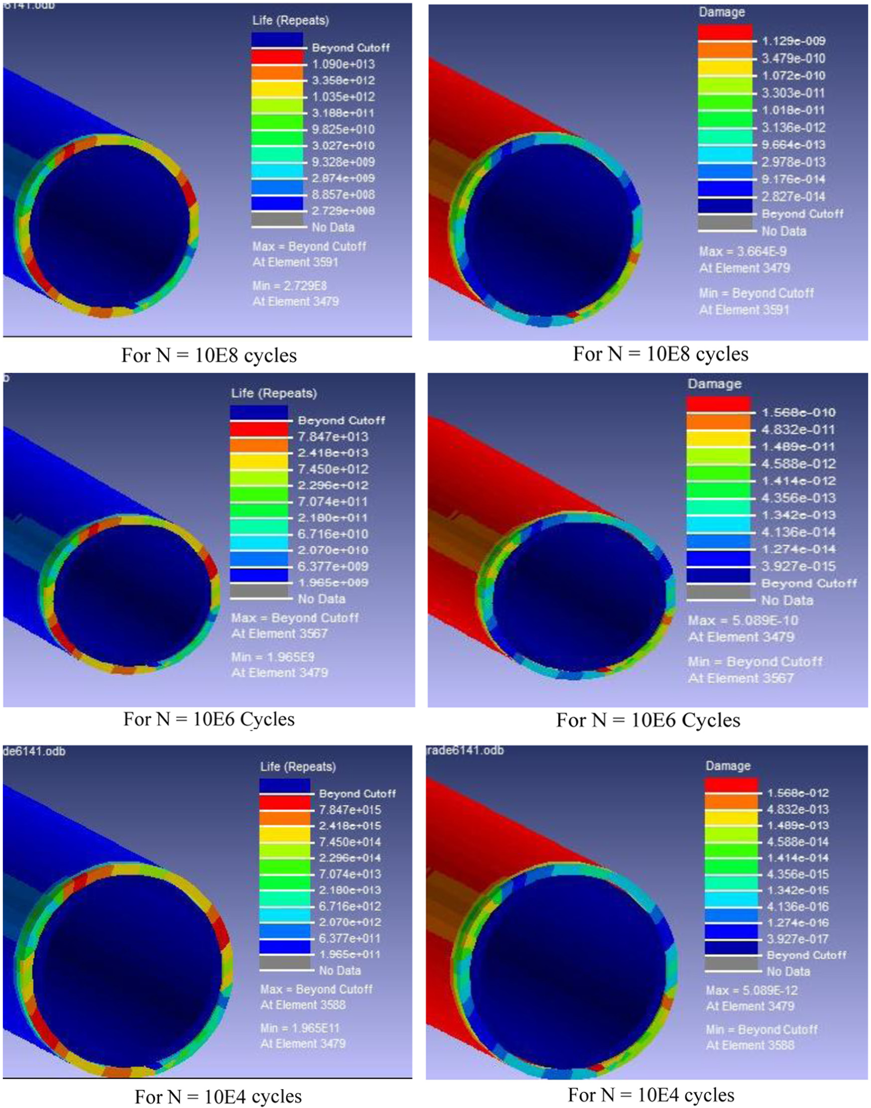
Life (seconds) and damage at the root joint for 10E2, 10E6, and 10E8 repeating cycles.

Conclusion and future work

The objective of this is to examine the structural response of a HAWT blade made of composite material to random wind loads. A reference wind turbine blade from Perkins and Cromack²⁵ was modeled in 3D CAD software and its natural frequency and static structural analysis results were first compared with the available results to check the accuracy of the modeling and static analysis. The modal frequencies and static structural results based on BEM approach were found to be very close to the reference, thus validating the model. After this, wind pattern for Salem city in Tamilnadu, India was calculated using three stochastic statistical methods—ARIMA, Markov chain, and Kalman filter. These models were developed based on the mean wind speed and the Weibull distribution data available in the reference for Salem city. Markov chain approach was selected due to its accuracy, and wind loads for 1 year were calculated for the predicted wind pattern using BEM method. These loads were used to perform fatigue analysis to calculate the fatigue life, damage, and safety factor. The variable stress vector due to wind loads was used to calculate rainflow matrix of stress amplitudes.

The authors conclude following:

This article presents an integrated methodology consisting of blade modeling, comparisons of long-term wind forecasting methods followed by forecasting of long-term wind speeds, aerodynamic load calculation and static, and fatigue analyses of composite HAWT blades for a site where limited or no raw wind data available for the site. It also analyzes conventional fatigue and CZM-based approach for root joint of blade. This end-to-end methodology is a unique contribution from authors in HAWT blade analysis.

It is found that the Markov chain model is an effective method to predict long-term wind speeds as compared to the ARIMA model which is more suitable for the short-term wind prediction. When the raw wind data are not available, Markov chain approach performs quite well in generating the synthetic wind as it does not need historical wind data as training data.

For fatigue analysis, the Markov chain–based wind prediction is found to be more effective as compared to ARIMA and Kalman spectrum because of higher variation in wind speeds leading to higher alternating stresses which influence fatigue. This effectiveness of Markov chain is found to be more in the months of higher mean speed.

The fatigue analysis results show that the critical area for blade failure is near the joint of the handle and the blade body. This is in line with various available studies on blade fatigue analysis.

CZM of the blade root is an effective method to analyze fatigue-induced debonding without the need to have initial crack.⁵⁷ However, in the current model, this method provided less conservative results, that is, higher available life. This is highly dependent on the properties of the interface elements and needs further study.

The smaller stress amplitudes contribute to the fatigue damage accumulation more than the high stress amplitudes.

The Epoxy S-Glass UD material is found to have better fatigue performance than E-Glass UD (QQ1) and carbon/glass-hybrid-fiber-reinforced epoxy (P2B) materials as it gives the highest fatigue life, better safety factor, and the lowest damage among the three materials for blade skin. It is also seen that Epoxy S-Glass UD material has least fatigue sensitivity for life and safety factor when load scale is varied from 0.25 to 2 as compared to QQ1 and P2B. P2B has the maximum sensitivity.

As an extension of this work, the authors propose to extend the modeling and analysis methodology developed in this article to large wind turbine blade with complex material layup in different parts of the blade such as the NREL 5 MW blade.⁵⁹ The authors plan to consider multiple input parameters such as pressure, humidity, and temperature and use newer methods such as ANN to predict mean wind speeds for long term. Authors would like to analyze effect of interface properties on the life and damage evolution using CZM approach. Finally, the authors would like to study the effect of variation of blade geometry, blade weight, and geospatial variation of wind loads on the fatigue life of this large blade.

Footnotes

Academic Editor: Aditya Sharma

Declaration of conflicting interests

The author(s) declared no potential conflicts of interest with respect to the research, authorship, and/or publication of this article.

Funding

The author(s) received no financial support for the research, authorship, and/or publication of this article.

References

Wang

et al . Aeroelastic coupling analysis of the flexible blade of a wind turbine. Energy 2015; 89: 1001–1009.

Liu

Liang

et al . Influence of the vibration of large-scale wind turbine blade on the aerodynamic load. Enrgy Proced 2015; 75: 873–879.

Liu

Liang

et al . Vibration-induced aerodynamic loads on large horizontal axis wind turbine blades. Appl Energ 2017; 185: 1109–1119.

Kaneko

Uehara

Senjyu

et al . An integrated control method for a wind farm to reduce frequency deviations in a small power system. Appl Energ 2011; 88: 1049–1058.

Smith

Ahlstrom

Zavadil

et al . The role of wind forecasting in utility system operation. In: IEEE power & energy society general meeting, 2009 (PES’09), Calgary, AB, Canadam, 26–30 July 2009, pp.1–5. New York: IEEE.

Yoon

. Numerical investigation on effects of rotor control strategy and wind data on optimal wind turbine blade shape. Wind Struct 2014; 18: 195–213.

Ghasemi

Jahanshir

Tarighat

. Numerical and analytical study of aeroelastic characteristics of wind turbine composite blades. Wind Struct 2014; 18: 103–116.

Lee

Kim

Han

et al . Active load control for wind turbine blades using trailing edge flap. Wind Struct 2013; 16: 263–278.

Chen

Lee

. Inverse active wind load inputs estimation of the multilayer shearing stress structure. Wind Struct 2008; 11: 19–33.

10.

Grujicic

Arakere

Pandurangan

et al . Multidisciplinary design optimization for glass-fiber epoxy-matrix composite 5 MW horizontal-axis wind-turbine blades. J Mater Eng Perform 2010; 19: 1116–1127.

11.

Choi

Zhupanska

et al . A new fatigue analysis procedure for composite wind turbine blades. In: 32nd ASME wind energy symposium, AIAA SciTech Forum, National Harbor, MD, 13–17 January 2014. Reston, VA: AIAA.

12.

Lecheb

Nour

Chellil

et al . Dynamic prediction fatigue life of composite wind turbine blade. Steel Compos Struct 2015; 18: 673–691.

13.

Choi

Kim

et al . Fatigue life prediction based on Bayesian approach to incorporate field data into probability model. Struct Eng Mech 2011; 37: 427–442.

14.

Barbounis

Theocharis

. A locally recurrent fuzzy neural network with application to the wind speed prediction using spatial correlationNeurocomputing 2007; 70: 1525–1542.

15.

Flores

Tapia

. Application of a control algorithm for wind speed prediction and active power generation. Renew Energ 2005; 30: 523–536.

16.

Lei

Luan

Jiang

et al . A review on the forecasting of wind speed and generated power. Renew Sust Energ Rev 2009; 13: 915–920.

17.

Amezcua

Munoz

Probst

. Reconstruction of gusty wind speed time series from autonomous data logger records. Wind Struct 2011; 14: 337–357.

18.

Box

GEP

Jenkins

. Time series analysis: forecasting and control. San Francisco, CA: Holden-Day, 1976.

19.

Jung

Broadwater

Current status and future advances for wind speed and power forecasting. Renew Sust Energ Rev 2014; 31: 762–777.

20.

Cadenas

Rivera

. Wind speed forecasting in the South Coast of Oaxaca, México. Renew Energ 2007; 32: 2116–2128.

21.

Sansui

Azami

Kamaruzzaman

. An initial review: stochastic application in wind speed forecasting. In: Zaharim

Panagopoulos

Zhang

et al . (eds) Recent advances in energy, environment and development, Cambridge, MA, 30 January-1 February 2013, pp.82–86. World Scientific and Engineering Academy and Society (WSEAS) Press.

22.

Negra

Holmstrøm

Bak-Jensen

et al . Model of a synthetic wind speed time series generator. Wind Energy 2007; 11: 193–209.

23.

Huang

. Prediction of typhoon design wind speed and profile over complex terrain. Struct Eng Mech 2013; 45: 1–18.

24.

Wang

et al . Aerodynamic loads and aeroelastic responses of large wind turbine tower-blade coupled structure in yaw condition. Struct Eng Mech 2015; 56: 1021–1040.

25.

Perkins

Cromack

. Wind turbine blade stress analysis and natural frequencies. Wind Energy Center Reports, Paper-11, 1978, http://scholarworks.umass.edu/cgi/viewcontent.cgi?article=1010&context=windenergy_report

26.

Carta

Ramirez

Velázquezc

. A review of wind speed probability distributions used in wind energy analysis: case studies in the Canary Islands. Renew Sust Energ Rev 2009; 13: 933–955.

27.

Yılmaz

Çelik

. A statistical approach to estimate the wind speed distribution: the case of Gelibolu region. DoğuşÜniversitesi Dergisi 2008; 9: 122–132.

28.

Wang

et al . Wind-induced responses and equivalent static wind loads of tower-blade coupled large wind turbine system. Struct Eng Mech 2014; 52: 485–505.

29.

Burton

Jenkins

Sharpe

et al . Wind energy handbook. 2nd ed.West Sussex: John Wiley & Sons, Ltd., 2011.

30.

Hansen

MOL

. Aerodynamics of wind turbines. 2nd ed.London: Earthscan, 2008.

31.

Tenguria

Mittal

Ahmed

. Structural analysis of horizontal axis wind turbine blade. Wind Struct 2013; 16: 241–248.

32.

Rafiee

Fakoor

. Aeroelastic investigation of a composite wind turbine blade. Wind Struct 2013; 17: 671–680.

33.

Vardar

Eker

. Mathematical modelling of wind turbine blades through volumetric view. Wind Struct 2006; 9: 493–503.

34.

Spagnoli

Montanari

. Along-wind simplified analysis of wind turbines through a coupled blade-tower model. Wind Struct 2013; 17: 589–608.

35.

Sriram

Krishnamohan

Gopalasamy

. Weibull parameters for wind speed distribution in Salem city. J Ind Pollut Contr 2004; 20: 53–58.

36.

Lakshmanan

Gomathinayagam

Harikrishna

et al . Basic wind speed map of India with long-term hourly wind data. Curr Sci India 2009; 96: 911–922.

37.

McNerney

Veers

. A Markov method for simulating non-Gaussian wind speed time series. Albuquerque, NM: Sandia National Laboratories, 1985.

38.

Choi

Cho

. Reliability-based design optimization of wind turbine blades for fatigue life under dynamic wind load uncertainty. Struct Multidiscip O 2016; 54: 953–970.

39.

Choi

Zhupanska

et al . Integrating variable wind load, aerodynamic, and structural analyses towards accurate fatigue life prediction in composite wind turbine blades. Struct Multidiscip O 2016; 53: 375–394.

40.

Zastrau

Schlaak

Bruns

et al . Differences in wind forecast accuracy in the German North and Baltic Seas. Int J Environ Sci Dev 2014; 5: 575–580.

41.

Karatepe

Corscadden

. Wind speed estimation: incorporating seasonal data using Markov chain models. ISRN Renew Energ 2013: 657437 (9 pp.).

42.

Shamsnia

Shahidi

Liaghat

et al . Modeling of weather parameters using stochastic methods (ARIMA model) (Case Study: Abadeh Region, Iran). In: International conference on environment and industrial innovation (IPCBEE), Kuala Lumpur, Malaysia, 17–19 June 2011, vol. 12. Singapore: IACSIT Press.

43.

Kalman

. A new approach to linear filtering and prediction problems. J Basic Eng: T ASME 1960; 1: 35–45.

44.

Yahya

. Turbines compressors and fans. New Delhi, India: Tata McGraw-Hill Education, 2010.

45.

Hoffman

Ramsay

Gregorek

. Effects of grit roughness and pitch oscillations on the NACA 4415 airfoil. Golden, CO, USA: National Renewable Energy Laboratory, 1996.

46.

Rajadurai

Christopher

Thanigaiyarasu

et al . Finite element analysis with an improved failure criterion for composite wind turbine blades. Forsch Ingenieurwes 2008; 72: 193–207.

47.

Salimi-Majd

Azimzadeh

Mohammadi

. Loading analysis of composite wind turbine blade for fatigue life prediction of adhesively bonded root joint. Appl Compos Mater 2015; 22: 269–287.

48.

Mandell

Samborsky

. SNL/MSU/DOE composite material fatigue database. Albuquerque, NM: Sandia National Laboratories, 2014.

49.

Mandell

Ashwill

Wilson

et al . Analysis of SNL/MSU/DOE fatigue database trends for wind turbine blade materials. Sandia report, SAND2010-7052. Albuquerque, NM: Sandia National Laboratories, 2010.

50.

Huh

Lee

Kim

et al . Effect of stress ratio on fatigue life of GFRP composites for WT blade. J Mech Sci Technol 2012; 26: 2117–2120.

51.

Roundi

El Mahi

El Gharad

et al . Experimental and numerical investigation of the effects of stacking sequence and stress ratio on fatigue damage of glass/epoxy composites. Compos Part B: Eng 2017; 109: 64–71.

52.

Gambone

. The effect of R-ratio on the mode II fatigue delamination growth of unidirectional carbon/epoxy composites. Doctoral Dissertation, The University of British Columbia, Vancouver, BC, Canada, 1991.

53.

Rahman

Kadirgama

Noor

et al . Fatigue life prediction of lower suspension arm using strain-life approach. Eur J Sci Res 2009; 30: 437–450.

54.

Samborsky

Wilson

Mandell

. Comparison of tensile fatigue resistance and constant life diagrams for several potential wind turbine blade laminates. J Sol Energy Eng 2009; 131: 011006.

55.

Kalkhoran

Salimi-Majd

Mohammadi

. Fatigue life prediction for adhesively bonded root joint of composite wind turbine blade using cohesive zone approach. In: Attaf

(ed.) Recent advances in composite materials for wind turbine blades, Hong Kong, 30 January–1 February 2013, pp.221–232. The World Academic Publishing Co. Ltd.

56.

Hosseini-Toudeshky

Jahanmardi

Goodarzi

. Progressive debonding analysis of composite blade root joint of wind turbines under fatigue loading. Compos Struct 2015; 120: 417–427.

57.

Khoramishad

Crocombe

Katnam

et al . Predicting fatigue damage in adhesively bonded joints using a cohesive zone model. Int J Fatigue 2010; 32: 1146–1158.

58.

Bak

Turon

Lindgaard

et al . A simulation method for high-cycle fatigue-driven delamination using a cohesive zone model. Int J Numer Meth Eng 2015; 106: 163–191.

59.

Jonkman

Butterfield

Musial

et al . Definition of a 5-MW reference wind turbine for offshore system development. Technical report no. NREL/TP-500-38060. Golden, CO: National Renewable Energy Laboratory, 2009.

Statistical wind prediction and fatigue analysis for horizontal-axis wind turbine composite material blade under dynamic loads

Abstract

Keywords

Introduction

Blade modeling and structural analysis

Blade specifications and modeling

Blade structural analysis

FEM of the blade

Natural frequency analysis

Static structural analysis

Wind field modeling and forecasting

Markov chain

Validation of Markov approach with a reference wind measurement

Application of Markov method for Salem location

ARIMA model

Kalman filter

Aerodynamic wind load calculation

Comparison of static load calculation by BEM method with analytical method

Blade fatigue analysis

Effect of stress ratio

Effect of stress criteria

Analysis with different skin materials

CZM of blade root joint

Conclusion and future work

Footnotes

Declaration of conflicting interests

Funding

References