
Abstract
As a methodology of resource location and allocation, reverse auctions are one of the most important activities in supply chains. There are four main auction mechanisms in auction theory, ascending-bid auctions, descending-bid auctions, first-price and sealed-bid auctions, and second-price and sealed-bid auctions. Recently, procurement bidding auctions have been widely studied in the aspects of bidding strategy, auction mechanism with different characteristics, behavior and psychology, collusion and its detection method, and the risk management. However, studies addressing the issue of which is the better reverse auction mechanism in cost-down performance are rarely documented. In this work, simulations are performed to study the integrated process of a dynamic online reverse auction and a static sealed-bid reverse auction using timed colored Petri nets based on the contribution of event management and workflow in Petri net theory. In the Petri net models, colored tokens represent bidders’ related data instantly, and transition nodes are in charge of executing bidding process rules whenever they are enabled. In addition, three programming methods including bidder’s bid and auctioneer’s winner set decision-making methods are embedded in the bidding process rules. Then, a hierarchical Petri net model is employed to compare cost-down range performance of dynamic online reverse auction and a static sealed-bid reverse auction, respectively. By modeling a comparison rule through a transition node, a reverse auction mechanism with better cost-down performance can be revealed based on the convergent simulation results.
Introduction
A supply chain composed of logistics, information flow, and capital flow is determined by reverse auctions, which have become an effective and efficient way of achieving lower acquisition costs, lower costs for new suppliers to enter a market, and consequently, better market efficiency. With the development of information technology, auction mechanisms have been greatly extended, for example, online auctions and online reserved auctions. A deluge of studies concentrating on the bidder’s bid-decision-making models using game theory and operation research methods are found in architecture and industrial engineering. However, in the field of supply chain management (SCM), little work on auctions is presented. There are also some kinds of sub-fields such as probability of winning, bidding behavior, information/risk effects, bidding strategies, and mechanisms. However, few of them combine buyers and sellers using object-oriented Petri net models into a common bidding environment which cannot accommodate a complicated actual bidding situation.
This research conducts two Petri net models for a static sealed-bid reverse auction and a dynamic online reverse auction, respectively. A bid-decision-making method, a winner-decision-making method, and an online price cut-down method are proposed. In order to reveal the result of a better auction mechanism, simulation data are given based on Petri nets. After running 2000 times, a better auction mechanism is found.
This article is organized as follows. Section “Literature review” presents a literature review on supply chains, auctions, and Petri nets. In sections “A static sealed-bid reverse auction model” and “A dynamic descending-bid online reverse auction model,” a static sealed-bid reverse auction and a dynamic online reverse auction Petri net models are studied, respectively. Section “A Petri net model for comparing two mechanisms” reports the contrastive simulation results and section “Conclusions” concludes this article.
Literature review
Auctions/bidding and supply chains
Due to practical, empirical, and theoretical reasons, auction theory is very important. First, a huge volume of economic transactions are implemented through auctions. Second, auction theory provides a valuable testing ground for economic theory. Third, it has been the basis of much fundamental theoretical work such as posted prices and negotiations. 1 McAfee and McMillan 2 define auctions as a market institution with an explicit set of rules determining resource allocation and prices based on bids from the market participants. Although many auctions define the environment of multiple bidders’ purchases from one seller, it is more common in actual transactions that a single buyer purchases commodity from multiple bidders. Actually, this research is conducted in the environment of the latter type. In other words, a single buyer chooses the optimal sellers from various auction participants in a supply chain.
There are four basic mechanisms of auctions. 1 The first two mechanisms are the ascending-bid auction and the descending-bid auction, and the second two mechanisms are the first-price sealed-bid auction and the second-price sealed-bid auction. In an ascending-bid auction, the price successively increases until only one bidder remains and wins the object at the final price. A descending-bid auction works exactly in an opposite way. A first-price sealed-bid auction and a second-price sealed-bid auction refer that each bidder independently submits a single private bid without seeing other bids, and the object is sold to the bidder who makes the highest bid and the second-highest bid, respectively. In the first two mechanisms, bidders can obtain the information, but the second two mechanisms cannot. Based on the definition of English auctions and Dutch auctions, the provider of the bids is the buyer which leads to the highest bid holder becoming the winner, while it should organize an auction involving multiple sellers submitting their bids if one buyer attempts to choose a vendor with the lowest price, and this kind of auction type is called reverse auctions in which the bid provider is changed from the buyers to the sellers. Reverse auctions can be a valuable tool that enhances buyer’s negotiation performance by raising the chance of obtaining better value of bids from vendors and optimizing the negotiation process. 3
Without loss of generality, there are five basic stages in a reverse auction. The first is the biding invitation process that calls for all of the potential suppliers discussing agreement intention about the threshold price, credit period, capacity, and lead time. The second is the bid process that includes the bid-decision-making and related data. Then, the next one is the bidding close process which specifies the ending rule of the second process such as the tender deadline or other rules. The forth is the bidding open process that ensures the open and fair justice of uncovering every bidder’s bid, and the last is a bidding evaluation process that executes by an auctioneer to decide the winner set. It should be stressed that a bidding object is the trade between a buyer and sellers. That is to say, the winner’s bid is the bidding object’s price that vendors sell to the buyer. This work addresses two reverse auction mechanisms basically with the same auction process associated with different sub-processes to compare their performance.
A lot of topics have been explored since 1960s such as optimal auctions, revenue equivalence, marginal revenues, risk preference, information effects, probability of winning, and related studies based on relaxing of many constraints. The earliest auction model is investigated by Friedman. 4 It is regarded as one of the most important bidding models working in the first-price sealed-bid auction, but many studies argue its strong restrictions and conduct a variety of models by relaxing constraints. 5 Gates, 6 Casey and Shaffer, 7 Hanssmann and Rivett, 8 Willenbrock, 9 and Morin and Clough 10 have offered improved models. Skitmore 11 tests four of the leading models by an empirical analysis of three large samples of real construction contract auction data and concludes that all the models produce rather poor predictions in both one-out and one-on mode.
With recent advances in information technology, online auctions have been born. They are different from the traditional paper form using internet as an auction transmission medium and database as bidding data repository. 12 It is very interesting that this work addresses the issues comparing a traditional auction with a modern one, sealed-bid with public-bid, private value with common value, static bidding with dynamic one, risk neutral context with risk aversion or seeking one, and stable bidding with jump bidding.13–15
Manufacturing supply chain networks (SCNs) are made up of complex interconnections among different manufacturing companies and service providers such as raw material suppliers, original equipment manufacturers (OEMs), logistics operators, warehouses, distributors, retailers, and customers. 16 A supply chain is a group of business entities working together for the same final product or service with its complementary contribution, cost, and profit. SCM represents one of the most significant paradigm shifts of modern business management by revealing that individual business no longer competes as solely autonomous entities, but rather as supply chains. 17 SCM is the active management of information flow, capital flow, logistics, and product flow in a supply chain to maximize customer value and achieve a sustainable competitive advantage. SCM has been defined as the design, planning, execution, control, and monitoring of supply chain activities with the objective of creating net value, building a competitive infrastructure, leveraging worldwide logistics, synchronizing supply with demand and measuring performance globally. 18 Most auctions are price driven and cost related with logistics, capacity management, inventories, credit period, and price-dependent demand. The results of auctions answer the following questions in SCM. Who is the seller/partner? What is the corresponding cooperative product? When and where do the parties execute the transaction? Why does a buyer choose these sellers? How many units are there in the transaction? How much is the object? As a result, reverse auctions have become one of the most important activities in SCM.
Petri nets
Petri nets 19 proposed by Carl Adam Petri have evolved into a formalism employed in different fields such as workflow, 20 evaluation and event management, 21 communication, 22 electronics, 22 chemistry logistics, 23 single-arm cluster tool with wafer revisiting, 24 manufacturing systems,25–41 and supervisory control of discrete event systems.42–47 Due to the limitations of the original paradigm of Petri nets, different extensions have been made, including the concept of time, colors, and hierarchical levels. A variety of types of Petri nets have been derived such as generalized stochastic Petri nets (GSPN), 48 timed Petri nets (TPN), 49 colored Petri nets (CPN), 50 colored timed Petri nets (CTPN), 51 batch deterministic stochastic Petri nets (BDSPN), 17 and deterministic and stochastic Petri nets (DSPN). 52 Accordingly, many simulation tools have been compiled such as INA, 53 TINA, 54 CPN, 50 and ExSpect. 55 Outmal et al. 56 analyzed closed-loop supply chain based on first-order hybrid Petri nets (FOHPN).
Specifically, CPN integrates the strengths of basic Petri nets with those of a high-level programming language. They are flourished to model systems in which communication, synchronization, and resource sharing play a critical role. Given a place node, all tokens must have token colors which belong to a specified type that is called color. 57 In CPN, each token is attached a color, presenting the identity of the token. A transition can fire with respect to each of its colors. The color attached to a token may be changed by a transition firing and it often represents a complex data value. 58
According to Jensen,
58
a CPN is defined as a five-tuple
Elements of
Figure 1 illustrates a CPN with a net structure, colored tokens, and transition rules.

A colored Petri net.
In the net structure, the initial marking is (2, 1, 0), where two colored tokens including 32 and 35 are in place
When timing information is added to a CPN model, CTPN can be constructed. A CTPN makes it possible to evaluate how efficiently a system performs its operations and it also makes possible to model and validate real-time systems, where the correctness of the system relies on the proper timing of the events. In addition, a CTPN is an extension of Petri nets able to cope with multiple processes and time constraints. A CTPN finds useful application in the modeling of systems characterized by a distributed and concurrent nature, by the synchronization among tasks that use shared resources. 59 The main difference between timed and untimed CPN models is that the tokens in a timed CPN model, in addition to the token color, can carry a second value, called a timestamp. This means that the marking of a place where the tokens carry timestamps is now a timed multiset, specifying the elements in the multiset together with their timestamps. A timed CPN model can always be transformed into an untimed CPN model by making all color sets untimed, removing all timestamps from initialization functions and removing all time delay inscriptions on arcs and transitions. The possible occurrence sequences of the timed CPN model always form a subset of those of its corresponding untimed CPN model. In other words, turning an untimed CPN model into a timed model cannot create new behavior in the form of new occurrence sequences.
Zhang et al. 57 present a detailed literature review on Petri-nets’ applications to SCM. The main research sub-fields are strategic competitiveness, firm-focused tactics, and operational efficiency. The strategic competitiveness includes the design of supply chains and competitive advantage assessment. Relationship development, integrated operations, logistics and transportation, and coordination are included in firm-focused tactics. Operational efficiency involves inventory management and control, production, planning and scheduling, information sharing, coordination and monitoring, and supply chain risk management. Nandula and Dutta 60 study an auction Petri net model with emphasis on manufacturing systems. So far, supply chain auctions have barely been explored using Petri nets. This research takes the attempt for modeling, analysis, and performance evaluation of a reverse auction process.
Petri net models have a good track record for performance validation of time-dependent concurrent processes, such as communication and messaging protocols, as demonstrated in Ma et al.61,62 and Viswanadham and Raghavan. 15 Based on the advantages of Petri nets, it is an approach to connect logistics, information flow, and capital flow. In addition, it can accurately represent reverse auction behavioral rules and implied event sequencing. The characteristics of concurrency, asynchronism, dynamics, and timed colored tokens demonstrate that Petri nets are one of the most suitable models to express the dynamic online reverse auctions which can be indicated visually and understandably based on the monitor of every time unit like a vidicon. In this work, colored tokens give a wonderful usage for many different and changing bidding data states of every bidder. In addition, colored tokens make a Petri net model structurally smaller than a non-colored one which is complex and unreadable. Simulations based on Petri nets can make bidding information interactivity, timeliness, just like which happens in a real scenario.
Contribution
Due to a large body of literature on Petri net applications to workflows in supply chains, this work attempts to introduce Petri nets to procurement auctions in supply chains. In this work, two Petri net models of a static sealed-bid reverse auction and a dynamic descending-bid online reverse auction embedded in several decision-making rules and colored tokens are constructed, respectively. In order to reveal a reverse auction mechanism with the better cost-down performance, a hierarchical Petri net model is set up. The flow of information in procurement auctions is accurately indicated by the flow of colored tokens with time constraints. In addition, a Petri net model of auctions graphically describes the reasons, the simulation results of every bidding activities, and the effects of bidding information on the decision of all bidding roles in every process.
A static sealed-bid reverse auction model
Assumptions
A real-world sealed-bid reverse auction process is very complex, and as a consequence, it is very important to grasp the main contradiction to analyze the essentials in this research. The following assumptions are stated as follows:
It is of information symmetry between bidders/sellers and of asymmetry between sellers and buyers. That is to say, every bidder only holds its private information business secret, and it cannot get any information of other competitors. However, a buyer knows some information that is unknown to bidders, such as the number of bidders, capacity of every bidder, and negotiated price.
The objective of every bidder is profit maximization.
Each rival is likely to bid as it has done in the past and the behavior is imperceptible and never changed by others.
It is admissible that a winner set must include the bidder with the lowest price, and the second lowest price may be a member of a winner set, which is dependent on the actual demand of the buyer and the capacity of every bidder.
Demand is price sensitive for every bidders and a buyer. Scale of demand is the quantity of contract which is the demand forecasting agreement of a long term, and a bidder predicts price-sensitive demand for more precise order.
Every bid is independent.
There is only one bidding object with multiple quantities in the reverse auctions.
In order to ensure the fairness of the cost-down range calculation, same capacities of each bidder have been put into two reverse auction mechanisms.
Each bidder is rational.
It is permitted that multiple winners can share an auction by executing their own bids.
The seller’s quantity of winning can be represented in function of the price-dependent demand.
Assumptions (1), (2), (6), and (9) ensure that the bid and winner-decision-making implemented in a private, rational, and profit maximization–based manner without any effects from others. Assumptions (3), (4), (5), (7), (10), and (11) provide some constraints of a static sealed-bid reverse auction model, and Assumption (8) guarantees the comparability between the current and last cost-down performances.
Notation
There are some notations as follows:
n is defined as the number of bidders with ID = 1,2, …, n;
Description of a static sealed-bid reverse auction process
There are five steps in this auction process. Figure 2 depicts a basic auction process and Figure 3 shows the bid and bidding close sub-processes in a static sealed-bid reverse auction.
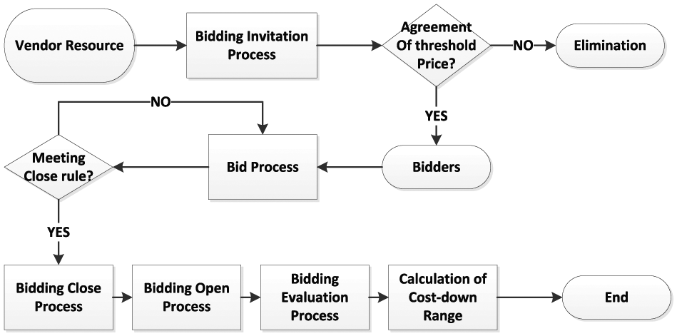
A basic auction process.

A static reserved sealed-auction bidding close process.
Step 1. There are a large number of vendors in a particular industry who are interested in a contract with their true cost, estimated industry average cost, capacity, last time winning price and share. In order to organize a valid bidding, a buyer invites every vendor to negotiate with price, capacity, credit period, etc.
Step 2: After negotiation before bid, the buyer divides all the vendors into two types. Type 1 consists of those whose negotiation prices are higher than the threshold price and Type 2 is opposite. Steps 1 and 2 are called the bidding invitation process.
Step 3. Auction begins with bidders belonging to Type 2 and ends at the stipulated time defined by the buyer. Every bidder presents its bid with a sealed form that ensures its bid is private information. This is called the bid process.
Step 4. When time is out (bidding close process), every bid is kept in the dark box (maybe a database), and no one could know all the bids until the buyer opens the box (bidding open process). After that, the buyer makes a winner-decision which minimizes the total cost. It is important to note that all the winners’ capacity should support the buyer’s demand, otherwise the shortage, trouble of vendor changing, price rise will ensue. This is called the bidding evaluation process.
Step 5. As the most important performance item, the cost-down range can be calculated by comparing the current price with the last one.
Petri net model of a static sealed-bid reverse auction
In this work, a Petri net approach is employed to formulate event rules and behavior process of reverse auctions by taking transition nodes to run the auction process rules and regarding timed colored tokens as process conditions/results. This model consists of a set of concurrent processes, each of which is formed by a number of temporally related tasks (segments). Tasks are executable by alternate resource sets including bidders and bundled bidding data. Time constraints are presented in the availability of each resource in resource sets and tasks in processes (Figure 4).

A Petri net model of a static sealed-bid reverse auction.
The interpretations of the Petri net are presented in Tables 1–4.
Interpretation of the places in the Petri net in Figure 4.

Interpretation of the transitions in the Petri net in Figure 4.

Colored value interpretation of the places in the Petri net in Figure 4.

Colored timed interpretation of transitions in Petri net in Figure 4.

Bid-decision-making method
Based on Assumption 2, the objective of every bidder is profit maximization. Therefore, profit function (objective function) should be output. From the view of bidders themselves, the actual cost is known. The unit profit is the difference between selling price/bid (

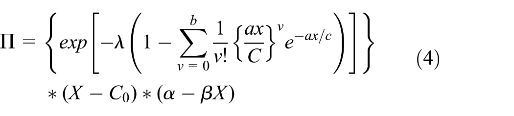
According to Friedman’s probability of winning,
4
the function

The winning of probability (
According to Dye and Hsieh, 63 the seller’s quantity of winning represented as a function of the price-dependent demand as indicated in Assumption (11) can be formulated as follows

where
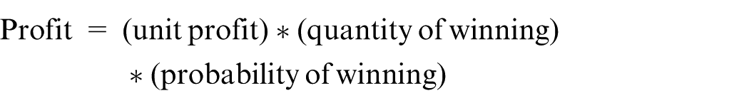
By equations (1)–(3), profit can be represented by
Note that the capacities should be enough to support corresponding winner share quantity, denoted by

Subject to

Winner-decision-making method
According to Step 5, every bidder’s bid is known by the buyer. As a result of the bid-decision-making method, the value of
First, the unit purchasing price should be calculated. Taking an example for consideration, two bidders bid with same value as US$4.5 and different credit periods. As a question, which one is better? The auctioneer converts the same two bids into “present net value,” denoted by

In a supply chain, every company not acting an end customer is both a buyer and a seller. The buyer’s downstream demand is also price dependent according to Assumption (11), and auctioneer’s purchasing price is decided by weighted average of winners’ bids, denoted by

where
Then, the total cost is defined as the purchasing cost for the product demand

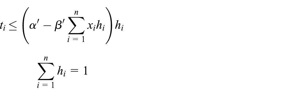
As for the constraints, the sum of every bidder’s winning share is equal to 1, that is,
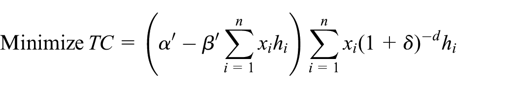
subject to
Finally, the cost-down range (CDR) issue is analyzed. The aim of the issue is to find out the difference between the current and last price. As a ratio, the difference should be divided by the last price, and the final result is found
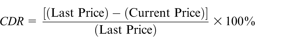
where the weighted average of last unit price is denoted by
Simulation results
To demonstrate the practical significance of the proposed approach, a detailed simulation experiment is conducted. We choose a typical group that can be divided into three sub-groups which consist of four bidders to illustrate the sensitivity with different initial values of
Three sub-groups’ state list in sealed-bid reverse auctions.

Simulation results of a sealed-bid reversed auction.

In Table 5,
A dynamic descending-bid online reverse auction model
A dynamic descending-bid online reverse auction becomes one of the most vivid cases of a supply chain modeled with Petri nets due to its asynchronism and concurrency. For the sake of simple descriptions, the Petri net model of a static sealed-bid reverse auction is called Model 1 in the following statement.
Assumptions
This model makes the following assumptions.
Unlike Model 1, although every bidder only holds its private information in this model, the information is actually the result of all bidders’ interaction of each other, from which every bidder can judge its own competitiveness and decide the next action. This is a common-value model in which a bidder’s value depends, to some extent, on other bidders’ signals.
In Model 1, the objective of every bidder is profit maximization. However, in an online reverse auction, profit maximization has been greatly weakened. 64 Priced risks may be excluded from the final bid to enhance competitiveness. As a result, the most interesting objective of bidders is to win the first ranking that ensures the probability of winning.
In share auctions, it is permitted that a winner set must include the bidder with the lowest price, and the second lowest price may be the member of a winner set, which is dependent on the actual demand of a buyer and the capacity of every bidder.
Demand is price sensitive for every bidders and a buyer.
Every bid is independent, but all bids have been inter-connected with each other to output the bidding price.
In single bidding object and multi-units, there is only one bidding object with multiple quantities in the reverse auctions.
In order to ensure the fairness of the CDR calculation, the capacity of each bidder is same as the last one.
Risk preference is dependent on corresponding context.
Online price-cut-down range of every bidder’s bid (value of
The moment that every bidder chooses to jump bid draws from a normal distribution.
Final bid is larger than the actual cost.
The effect of risk preference on the value of
Each bidder is risk neutral during the preheat phase, and then, risk preference changes during the jump auction phase.
It is permitted that multiple winners can share an auction by executing their own bids.
Assumptions (3), (4), (6), (7), and (14) are same as corresponding assumptions in Model 1 and they ensure the comparability of these two models. Assumptions (1) and (5) set the context of common-value with bidders’ interaction of each other in which the information effects on bidder’s behavior can be revealed. Assumption (2) can be regarded as the result of Assumption (1) that describes the objective of bidders in such a context. Assumptions (8), (9), (10), (11), (12), and (13) provide several constraints of a dynamic descending-bid online reverse auction model.
Notation
In addition to the notation of Model 1, in this model, several special variables are defined.

Figure 5 illustrates the whole process of a dynamic descending online reverse auction that has a maximum bidding time divided into the preheat phase and the hot jump auction phase. Every bidder has the equal opportunity of bid time, only if more than one new price has the ability to begin the next phase/sub-phase which can be called a beginning rule. There are several sub-phases with small bid time in a hot jump auction to prompt the competitiveness. Every bidder can find instant information of its bid including present ranking (variable
Steps 1, 2, and 3 are exactly as same as a static sealed-bid reverse auction process, which ensures the comparability of the two mechanisms of reverse auctions.
Step 4. Since the negotiation price is generally lower than the last winning price, ideally, new price can be born during the preheat phase. Stemming from the beginning rule, the next phase begins. On the condition of no new price, the reverse auction goes to end with the result of failure, which represents the bad organization of a pre-auction. In order to keep larger cost-down space, most of bidders choose to bid at the price approximately equating to negotiation value during the preheat phase.
Step 5. Eligible bidders with new price begin to enter the hot jump auction phase. During the first sub-phase with small left bidding time, bidders begin the war of price. As a result, new price has born, leading to the second sub-phase, cycling, and so on until the phase or sub-phase ends. It can be regarded as an iterative pattern that allows bidders to learn about their rivals’ valuations through the bidding process, which might lead them to adjust their own valuations.
Step 6. Dynamic auctions continue until the auction deadline is reached. Like a static sealed-bid reverse auction, no one could know all the bids until the buyer opens the data box. After that, the buyer makes a winner-decision which minimizes the total cost. It is worth noting that all the winners’ capacity should support the buyer’s demand. Otherwise, supply shortage, trouble of vendor changing, and price rise of a supply chain will be turn out.
Step 7. Same as Step 6 of a static sealed-bid reverse auction process, the CDR can be calculated using current and the last price and finds simulation results.

Bid process of a dynamic online reverse auction.
Petri net model of a dynamic descending-bid online reverse auction
After description of a dynamic descending-bid online reverse auction process, a Petri net model is constructed. Similar to the Petri net model of a static sealed-bid reverse auction, the model to be constructed employs transition nodes executing the reverse auction activities (e.g. invitation, bid-decision, and winner-decision) and timed colored tokens acting as the conditions or results. The flow of tokens of a given color in the Petri net model represents the bidder’s bidding data in every bidding process. Transition nodes corresponding to every bidding process are deterministic or stochastic. The firing of the transition nodes causes the sending of messages to its controller for the activities of the corresponding real task instance; the expiring of the transition can be driven by the completion of the task instance, via messages coming to the transition from its controller.
The data in Tables 7–10 are used to interpret the Petri net in Figure 6.
Interpretation of the places in the Petri net in Figure 6.

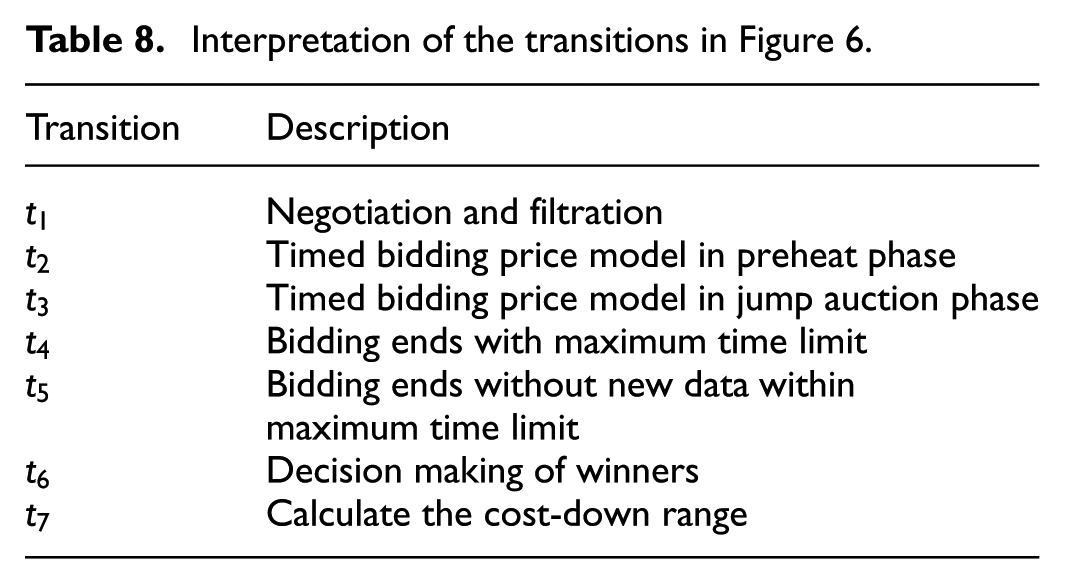
Interpretation of the transitions in Figure 6.
Colored value interpretation of the places in the Petri net in Figure 6.

Colored timed interpretation of transitions in Figure 6.


Petri net model of a descending-bid online reverse auction.
Bid cut-down method
According to Tversky and Kahneman,
65
risk choice-framing effect demonstrates that people tend to become risk aversion when getting benefit. On the contrary, they tend to become risk seeking when facing loss. There is no doubt that bidders tend to win the first ranking which guarantees their probability of winning. Therefore, reaching the first ranking is the best result for every bidder. At the same time, ranking going backwards and few bidding time left belongs to bad result that bidders are unwilling to face.
65
In order to get profitable situation, deciding how much to bid and how much to cut down at each time becomes the crucial choices. In other words, after one bidder’s first bid, the most important following behavior is to choose how much one should cut down to reach the first ranking, and here, the cut-down range is represented as
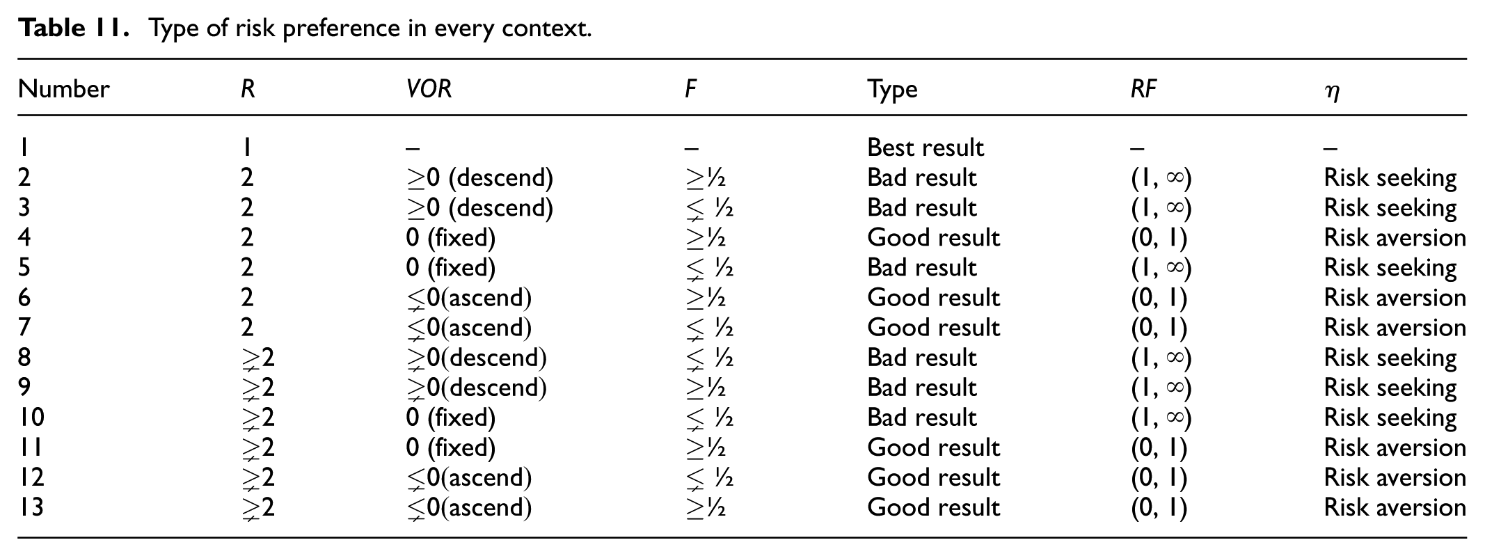
Apart from the best result aforementioned, it is profitable for a bidder to face the good result of rankings going forward and long rest time, while the reverse situations are bad result that a bidder is unwilling to meet. It is necessary to introduce the good result with the most unprofitable effects and the bad result with the most profitable ones, they are corresponding the Type 12 and Type 2 in Table 11, respectively. As the information of Type 10 shown in Table 11, good result is that the ranking has been maintained, while its ranking of only next-to-last with almost deadline time reached are very unprofitable to the bidder. As a reversed context just as Type 2 in Table 11, bad result is that the ranking has descended, while the second ranking with a lot of time left are profitable to the bidder. It is worthy to emphasize that the value of
Type of risk preference in every context.
It is understandable that new price is equal to the last price minus the step size, that is

According to Assumptions (9) and (12), the price-cut-down range (
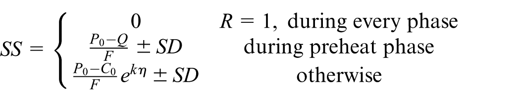
subject to
Actually, based on the assumptions aforementioned,
Maximum time limit
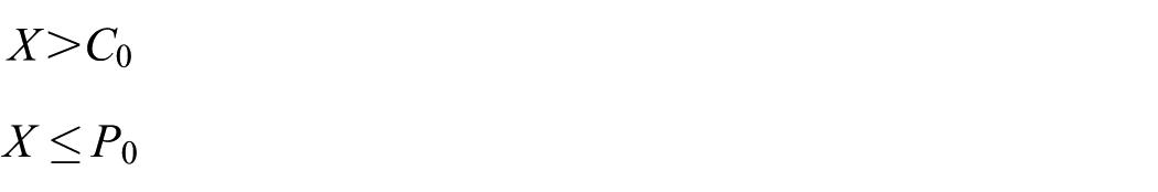
It is an interesting problem to decide optimal simulation time by the buyer. The simulation results of the proposed Petri net model provide a satisfactory explanation shown in Figure 7.
Cost-down range with change in the maximum time limit.
The maximum time limit has been settled from 8 to 100 in this plot on the horizontal axis. The curve becomes smooth after
Simulation results
Unlike a static sealed-bid reverse auction, Table 6 is completely unable to describe the whole process of online bidding because of a large quantity of dynamic and timed bidding process data.
Numerical results begin with dynamic data, and then, a final static result of a winner set will be given. In order to make the plot clear,

The first sub-groups’ state list in an online reverse auction.
The first sub-groups’ state in an online auction with timed ranking.

The second sub-groups’ state in online reverse auction.
The second sub-groups’ state in an online auction with timed ranking.

The third sub-groups’ state list in an online auction.

The third sub-groups’ state in an online auction with timed ranking.
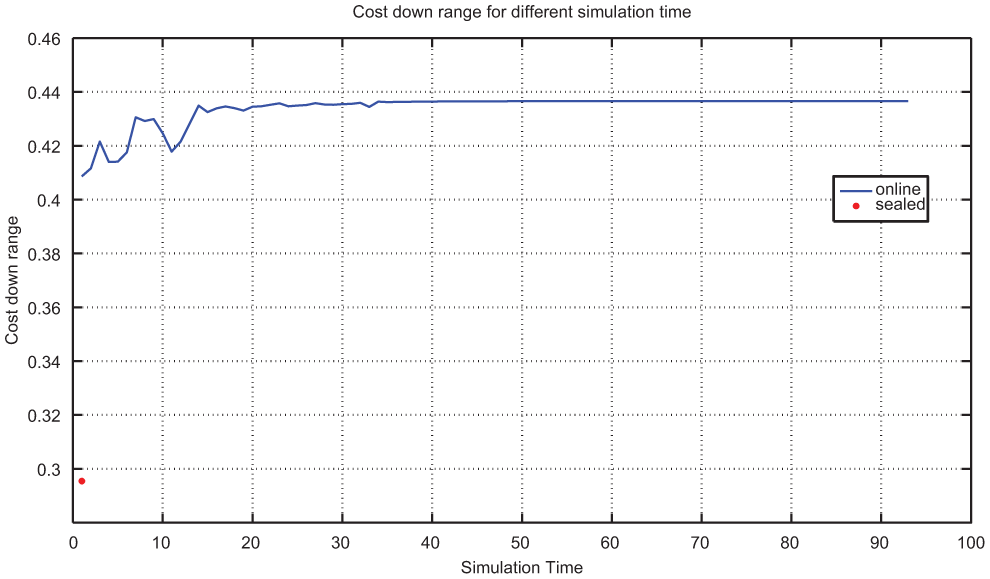
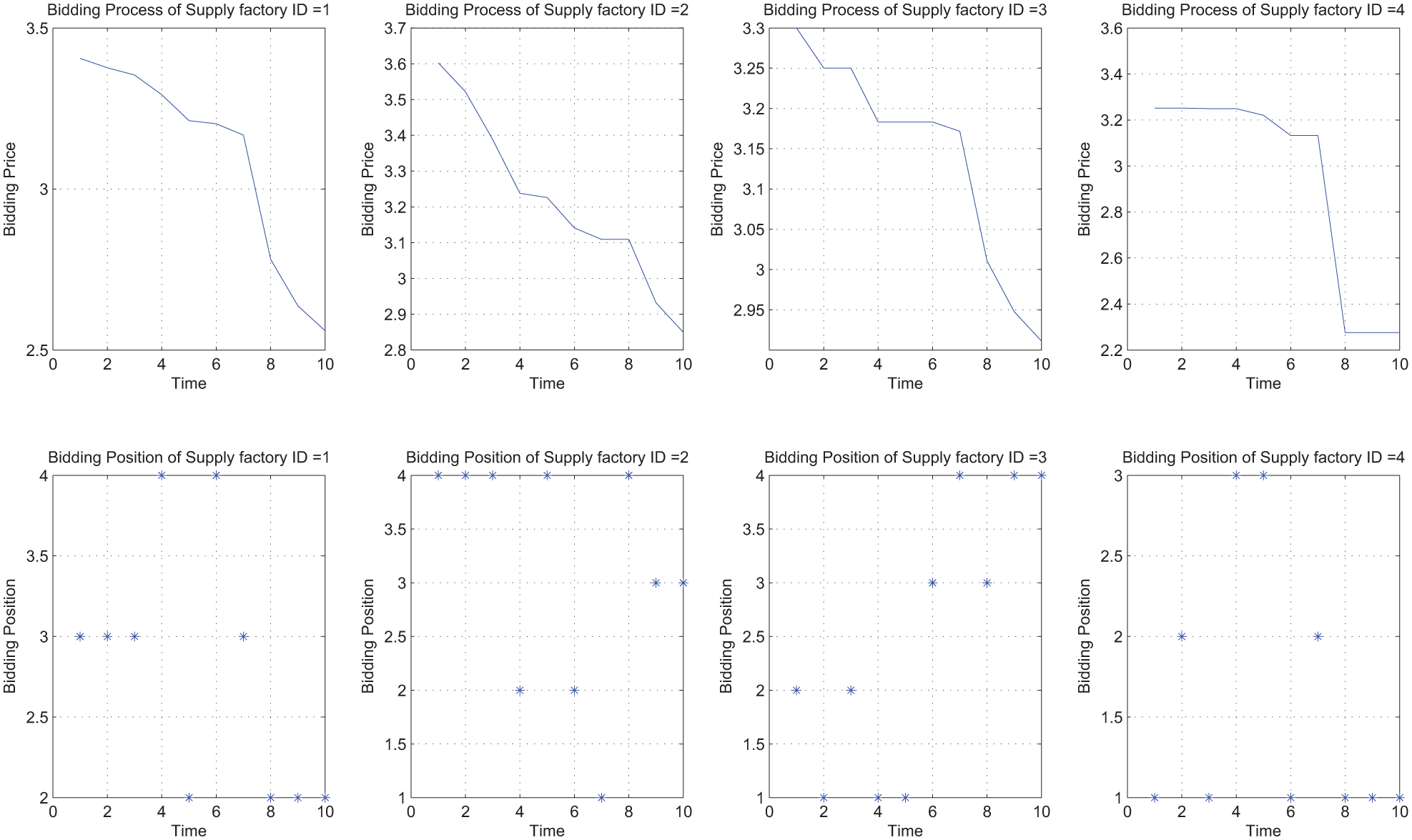
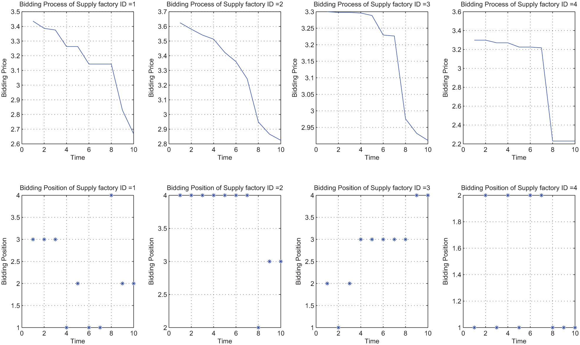
During the preheat phase and the jump bid phase, Figures 8, 10, and 12 illustrate the bid varying curves of the first, the second, and the third sub-groups, respectively. Four bidder’s bid curves go down slowly until the jump bid moment begins. During the jump bid phase, they are brought into playing a price war, and as a consequence, the bid varying curves become abruptly descending. When the deadline time reached, bid activities are stopped with the ultimate price fixed.
In order to understand every bidder’s bid in each time, Figures 9, 11, and 13 describe the bid varying curves and corresponding price value of the first, the second, and the third sub-groups, respectively. There are eight boxes in this type of plots, among which, the four boxes above are every bidder’s bid varying curves and corresponding boxes below are precise price value represented by a scatter chart.
These figures vividly replay the token games during the bidding process, from which we can reach a conclusion of information effects on bidder’s behavior in a common-valued manner. The timed CPN model simulates the dynamics and concurrent activities of a dynamic online reverse auction.
A Petri net model for comparing two mechanisms
After introducing the two different mechanisms of reverse auctions, this section analyzes which type has the better cost-down performance.
A hierarchical Petri net model is used to compare the CDR performance of a static sealed-bid reverse auction with that of a dynamic online reverse auction. Specially, the output place
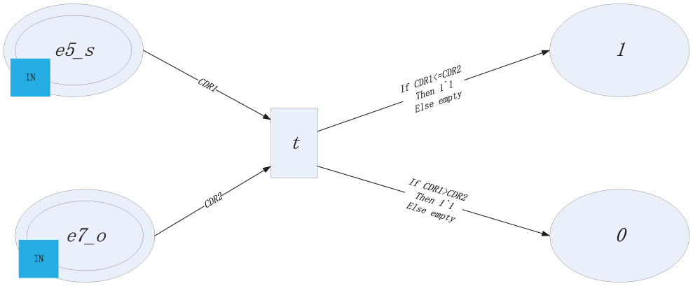
Comparing
According to 2000 simulation results, the numbers of tokens in place “1” and place “0” are 2000 and 0, respectively. It is shown that the performance of a dynamic online reverse auction dominates a static reserved sealed-bid reverse auction based on all the assumptions aforementioned. As a result, a dynamic online reverse auction is the better mechanism for cost-down performance; however, in a dynamic online reverse auction mechanism, a player will bid a little more aggressively which strengthens the opponent’s winner’s curse.
Conclusion
In this research, CTPN is used as the modeling technique embedded in several programming methods to analyze two reverse auction mechanisms. The token games play five bidding processes employing transition nodes acting reverse auction activities and timed colored tokens representing the bidding data, and then, the performances of two reverse auction mechanisms are obtained that can be compared with each other to find a dominant mechanism. As a powerful modeling tool, Petri nets present the bidding behavior, bidding data, bidding information circumstance, and bidding decision-making. In this research, Petri nets are used to study the integrated process of a dynamic online reverse auction and a static sealed-bid reverse auction. Similar with other methods, Petri nets can reach the optimization solution, but the superiority of Petri nets is the strong simulation ability for the whole process of procurement bidding auction which makes the discrete event in a supply chain to become traceable and controllable. Meanwhile, multiple bidding data from various bidders can be described by a simple auction Petri net while using CTPN. Moreover, the structure and scale of the Petri net will not be affected by adding a similar bidder conditional on the fixedness of transition rule, which makes this network extendable. In fact, auction is only one part of SCM, which is involved with multiple corporations, data, and discrete events. In the discrete event of SCM, the party involved and interactive data can be clearly illustrated in terms of Petri net models, which help promoting the strategy and the mode of SCM, coordination, and process control. Petri net can also be used more widely in SCM. Apparently, this research can be extended in the future, for example, relaxing strong constraints and taking multiple objective bidders and multiple subjects into account for every bidder.
Footnotes
Acknowledgements
The authors greatly appreciate the reviewers’ suggestions and the editors’ encouragement.
Academic Editor: Jiin-Yuh Jang
Declaration of conflicting interests
The author(s) declared no potential conflicts of interest with respect to the research, authorship, and/or publication of this article.
Funding
The author(s) disclosed receipt of the following financial support for the research, authorship, and/or publication of this article: This work was supported by Science and Technology Development Fund, MSAR, under Grant No. 078/2015/A3.