Sage Journals: Discover world-class research

Abstract

The main objective of this article is to propose a practical methodology to compute the induced curvature parameters for a line-conjugated tooth surface couple based on the normal vector of its instantaneous contact line. The computing formulae in different form are thus suggested for the preceding normal vector in order for convenient use. Based on this, the formulae for the induced curvature parameters are accordingly given out. Compared to the previous work, the deducing process is more rigorous and more laconic, and the obtained results are more practical. Concurrently, different deducing techniques are provided, and this is beneficial for the development of the meshing theory for gear drives. The theory and method presented are applied to the modified Hindley worm drive, and its basic and important equations are attained. The concrete numerical example is a type I drive, whose conjugate zone is divided into two parts. In one part, the value of the induced principal curvature is much smaller than that in the other one. The biggest induced principal curvature comes into view about at the inlet portion of the worm, and certainly the highest contact stress between the teeth will happen consistently at that position.

Keywords

Normal vector of instantaneous contact line induced normal curvature induced geodesic torsion line-conjugate surfaces Hindley worm drive

Introduction

As for a line-conjugate tooth surface couple, the induced normal curvature means the difference between the normal curvatures of its two tooth surfaces along a common tangential direction at an instantaneous meshing point on an instantaneous contact line. The induced principal curvature is the principal value of the induced normal curvature. The second surface, that is, the enveloped surface, in a line-conjugate surface couple essentially is the envelope to a one-parameter surface family, which is formed by the first surface, that is, the enveloping surface, under the given relative motion. Therefore, the induced normal curvature can completely be determined by the geometry of the enveloping surface and the relative motion of the surface couple. That is to say, the curvature parameters of the enveloped surface, even its equation, are not required to be known when computing the induced normal curvature. This is the reason why a word “induced” is put into the phrase “induced normal curvature.”

In the literature, a similar concept to the induced normal curvature is the relative normal curvature or the relative curvature for short. Generally speaking, the relative curvature means the difference of the normal curvatures of two surfaces in tangential contact along a common tangential direction. The two surfaces may stay in the line or point contact and the enveloping relation does not have to exist between them. Hence, the relative curvature needs to be obtained from the normal curvatures of the two surfaces in tangential contact. Thus, it can be seen that the induced normal curvature can be viewed as a special case of the relative curvature.

By definition, the induced normal curvature reflects the proximity degree of the two tooth surfaces along their common tangential direction and the curvature relation of the two line-conjugate surfaces. Therefore, the induced normal curvature has been found a broad application in the gear industry, which probably lies in the following three aspects. First, when making the adjustment computation for machining a spiral bevel or hypoid gear with curved teeth, the induced normal curvature can be used as the ground to avoid the interference.^1,2 Second, according to the Hertz formula in the contact mechanics, the induced normal curvature can be utilized to measure the contact stress level indirectly.^3,4 Third, in accordance with the Dowson formula in the theory of elasto-hydrodynamic lubrication, the film thickness of the lubricating oil at a transient meshing point can approximately be evaluated by means of the induced normal curvature.⁵

Due to the important applications mentioned above, how to compute the induced normal curvature began to be studied very early. Wildhaber⁶ and Baxter⁷ investigated the induced normal curvature for spatial gear drives from the point of view of the meshing theory based on the reference cone. In 1969, Dyson⁸ published a monograph on the kinematics and geometry of gear pairs, in which the relative curvature computation is touched. In the 1970s, Chen⁹ researched the induced normal curvature by employing the vector rotation method. Almost at the same time, Sakai¹⁰ performed an investigation on the induced normal curvature by employing the binary vector method.

About since the 1960s, Litvin¹¹ started to research the curvature relation of the line-conjugate tooth surfaces. Originally, he proposed the formula to calculate the induced normal curvature, whose precondition for application is to know the normal curvature of the generated surface. After entering the 21st century, he brought forward to calculate the induced normal curvature by means of the curvature parameter matrix.¹²

In 1985, Wu and Luo¹³ suggested a general formula to compute the induced normal curvature. In their formula, the derivative of the time with respect to the arc length is included. Afterward, a number of their followers^14–19 investigated the computation of the induced normal curvature by virtue of the relative differential technique.

In 1986, Chen²⁰ obtained a computing formula for the induced normal curvature by employing the rotation matrix. A little later, Dong²¹ simplified the formula achieved for calculating the induced normal curvature and put forward a more utility method to figure down the normal vector of the instantaneous contact line.

In the 1990s, Dooner and Seireg²² studied the computation of the induced normal curvature by exploiting the screw theory. In the mean time, Chen²³ studied the computation of the induced normal curvature. In 2012, Dong et al.²⁴ studied the induced normal curvature of the planar gearing transmission. Also in 2012, Radzevich²⁵ introduced the concept of the relative normal curvature to aid the computation of the Hertz stress for a gear drive in his treatise.

Similar to the induced normal curvature, the induced geodesic torsion can be defined as the difference of the geodesic torsions of the two line-conjugate tooth surfaces along a common tangential direction at an instantaneous meshing point. The induced geodesic torsion can be employed to determine the induced principal direction and thus the relevant induced principal curvature can be obtained for a line-conjugate surface couple further. In the literature,^{13–15,17,20–21} the computing formulae for the induced geodesic torsion were established on the strength of the induced normal curvature.

The aim of this article is to propose a methodology to compute the induced curvature parameter for a line-conjugated tooth surface couple based on the normal vector of its instantaneous contact line. The involved induced curvature parameters include the induced normal curvature, the induced geodesic torsion, the induced principal direction, and the induced principal curvature. In order to illustrate the theory and methodology suggested, the computation of the induced curvature parameters for the modified Hindley worm drive is taken to be an example. The meshing performances of a modified Hindley worm drive are not going to be expounded here because the elaborative exposition in this aspect may obviously be far beyond the scope of this article.

As reported by Buckingham²⁶ and Crosher,²⁷ the Hindley worm drive was initially invented circa in 1765 by Henry Hindley. About in 1909, Samuel I Cone greatly boosted the Hindley worm drive and got his related patent in 1932.^28–30 The basic design and manufacture methods of the Hindley worm drive were preliminarily summarized in the literature.³¹

Beginning from the 1980s, some authors^{13,14,32–34} researched the computation of the induced normal curvature for the Hindley worm drive. Among them, only Hu et al.³² provided the numerical results.

In the research of Dong,³⁵ the calculation of the induced normal curvature is contained and plenty of numerical examples are supplied. His work is based on the theory of locus surface.

In this work, the curvature parameters of the screw surface of the modified Hindley worm are attained via differentiating the surface equation directly. The normal vector of the instantaneous contact line of the modified Hindley worm pair is represented by means of the moving frame approach. The most important induced curvature parameters, namely the induced principal curvature, of the modified Hindley worm gearing are acquired by taking advantage of the normal vector of the instantaneous contact line. The numerical results are provided for verification and validation.

Equation of generated tooth surface and partial derivatives of meshing function

As shown in Figure 1, a fixed coordinate system $σ {O; \vec{i}, \vec{j}, \vec{k}}$ represents the static space. Simultaneously, two movable coordinate systems, $σ_{1} {O_{1}; {\vec{i}}_{1}, {\vec{j}}_{1}, {\vec{k}}_{1}}$ and $σ_{2} {O_{2}; {\vec{i}}_{2}, {\vec{j}}_{2}, {\vec{k}}_{2}}$ , are rigidly associated with the two line-conjugate tooth surfaces, $Σ_{1}$ and $Σ_{2}$ , respectively. In $σ_{1}$ , the equation of $Σ_{1}$ can be represented as

{\vec{r}}_{1} = {\vec{r}}_{1} (u, θ)

(1)

where $u$ and $θ$ are the two parameters of $Σ_{1}$ . In the usable region of $Σ_{1}$ , there is no singular point.

Figure 1.

Line-conjugate surface couple.

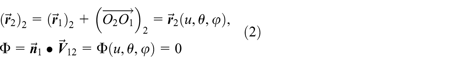
When the gear 1 revolves around its axis with the angle velocity $| {\vec{ω}}_{1} | = 1 rad / s$ , its tooth surface $Σ_{1}$ forms a one-parameter family of surfaces, ${Σ_{1}}$ , in the fixed space $σ$ . When the rotation angle of the gear 1 is $φ$ , the tooth surfaces $Σ_{1}$ and $Σ_{2}$ are in contact along an instantaneous contact line $L_{t}$ and the tooth surface $Σ_{2}$ of the gear 2 essentially is the envelope to ${Σ_{1}}$ . Therefore, the equation of $Σ_{2}$ can be represented as^12,13,21

\begin{array}{l} {({\vec{r}}_{2})}_{2} = {({\vec{r}}_{1})}_{2} + {(\vec{O_{2} O_{1}})}_{2} = {\vec{r}}_{2} (u, θ, φ), \\ Φ = {\vec{n}}_{1} • {\vec{V}}_{12} = Φ (u, θ, φ) = 0 \end{array}

(2)

where $Φ (u, θ, φ)$ is the so-called meshing function. Herein ${\vec{n}}_{1}$ and ${\vec{V}}_{12}$ separately are the unit normal vector of $Σ_{1}$ and the relative motion velocity of the surface couple at the transient meshing point $P$ on the instantaneous contact line $L_{t}$ , whose expressions are^13,21

\begin{array}{l} {\vec{n}}_{1} = \frac{{\vec{r}}_{1 u} \times {\vec{r}}_{1 θ}}{| {\vec{r}}_{1 u} \times {\vec{r}}_{1 θ} |}, {\vec{V}}_{12} = {\vec{ω}}_{12} \times {\vec{r}}_{1} \\ - {\vec{ω}}_{2} \times \vec{O_{2} O_{1}} + \frac{d}{d t} \vec{O_{2} O_{1}} \end{array}

(3)

where ${\vec{ω}}_{2}$ is the angle velocity of the gear 2, ${\vec{ω}}_{12}$ is the relative angle velocity of the surface couple, and ${\vec{ω}}_{12} = {\vec{ω}}_{1} - {\vec{ω}}_{2}$ . Under the assumption that $| {\vec{ω}}_{1} | = 1 rad / s$ , $φ = t$ and $d φ = dt$ , in which the notation $t$ denotes the time.

In the conjugate zone, the relationship between the unit normal vectors, ${\vec{n}}_{1}$ and ${\vec{n}}_{2}$ , of $Σ_{1}$ and $Σ_{2}$ is ${\vec{n}}_{2} = {\vec{n}}_{1}$ . In the light of the relative differential method,¹³ it is possible to have

d_{2} {\vec{r}}_{2} = d_{1} {\vec{r}}_{1} + {\vec{V}}_{12} d φ, d_{2} {\vec{n}}_{2} = d_{1} {\vec{n}}_{1} + {\vec{ω}}_{12} \times {\vec{n}}_{1} d φ

(4)

where the notation, $d_{m} (•)$ , denotes the relative differentiation within $σ_{m}$ , $m = 1, 2$ .

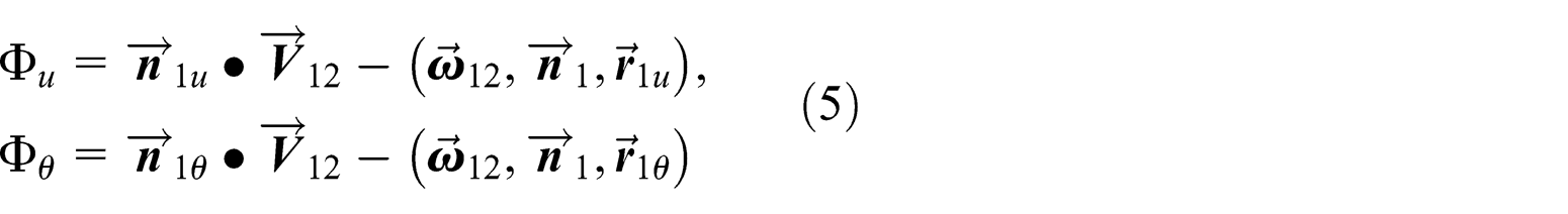
The three partial derivatives of $Φ$ can be procured as

\begin{array}{l} Φ_{u} = {\vec{n}}_{1 u} • {\vec{V}}_{12} - (\vec{ω_{12}}, {\vec{n}}_{1}, {\vec{r}}_{1 u}), \\ Φ_{θ} = {\vec{n}}_{1 θ} • {\vec{V}}_{12} - (\vec{ω_{12}}, {\vec{n}}_{1}, {\vec{r}}_{1 θ}) \end{array}

(5)

Φ_{φ} = {\vec{n}}_{1} • [{\vec{V}}_{12} \times {\vec{ω}}_{1} + {\vec{ω}}_{12} \times ({\vec{ω}}_{1} \times {\vec{r}}_{1}) + \vec{C}]

(6)

where $\vec{C} = \frac{d {\vec{ω}}_{12}}{d φ} \times {\vec{r}}_{1} - \frac{d {\vec{ω}}_{2}}{d φ} \times \vec{O_{2} O_{1}} - {\vec{ω}}_{2} \times \frac{d \vec{O_{2} O_{1}}}{d φ} + \frac{d^{2}}{d φ^{2}} \vec{O_{2} O_{1}}$ . $Φ_{φ}$ is called the meshing limit function or the limit function of the second kind,^13,21 which is often reaped by taking the ordinary partial derivative of $Φ$ in a specific meshing analysis as well.

Owing to $d Φ = 0$ in the conjugate zone, from equation (5), it is easy to have

Φ_{φ} d φ = ({\vec{ω}}_{12}, {\vec{n}}_{1}, d_{1} {\vec{r}}_{1}) - {\vec{V}}_{12} • d_{1} {\vec{n}}_{1}

(7)

Singular point condition of envelope and elicitation of normal vector of instantaneous contact line

Singular point condition of envelope

Obviously, the singular point condition for $Σ_{2}$ may be represented as $d_{2} {\vec{r}}_{2} = 0$ . Under this condition, from the first expression in equation (4), it is easy to acquire

{\vec{r}}_{1 u} du + {\vec{r}}_{1 θ} d θ = - {\vec{V}}_{12} d φ

(8)

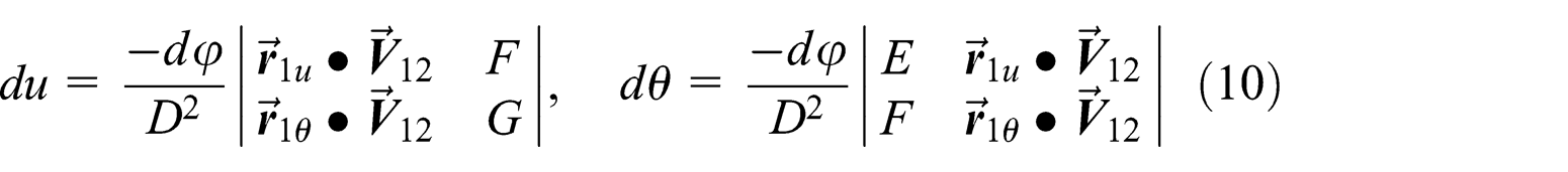
Making the dot product on the both sides of equation (8) with respect to ${\vec{r}}_{1 u}$ and ${\vec{r}}_{1 θ}$ , respectively, yields a system of linear equations in regard to $du$ and $d θ$ , which can be expressed as

{\begin{matrix} Edu + Fd θ = - {\vec{r}}_{1 u} • {\vec{V}}_{12} d φ \\ Fdu + Gd θ = - {\vec{r}}_{1 θ} • {\vec{V}}_{12} d φ \end{matrix}

(9)

where $E$ , $F$ , and $G$ are the coefficients of the first fundamental form for $Σ_{1}$ . That is to say, $E = {\vec{r}}_{1 u} • {\vec{r}}_{1 u}$ , $F = {\vec{r}}_{1 u} • {\vec{r}}_{1 θ}$ , $G = {\vec{r}}_{1 θ} • {\vec{r}}_{1 θ}$ .

Solving equation (9) gives rise to

du = \frac{- d φ}{D^{2}} | \begin{matrix} {\vec{r}}_{1 u} • {\vec{V}}_{12} & F \\ {\vec{r}}_{1 θ} • {\vec{V}}_{12} & G \end{matrix} |, d θ = \frac{- d φ}{D^{2}} | \begin{matrix} E & {\vec{r}}_{1 u} • {\vec{V}}_{12} \\ F & {\vec{r}}_{1 θ} • {\vec{V}}_{12} \end{matrix} |

(10)

where $D^{2} = EG - F^{2}$ .

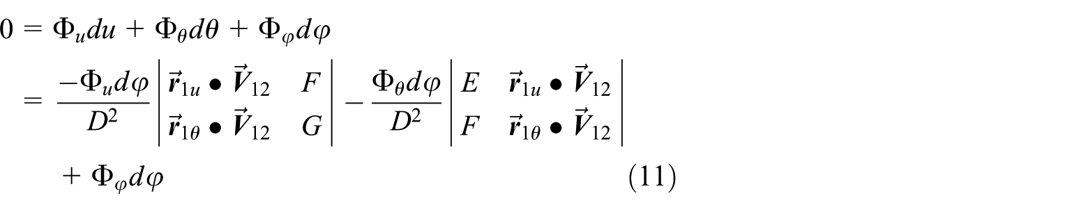
Conducting the total differential to the meshing equation $Φ (u, θ, φ) = 0$ and taking advantage of equation (10) lead to

\begin{array}{l} 0 = Φ_{u} d u + Φ_{θ} d θ + Φ_{φ} d φ = \frac{- Φ_{u} d φ}{D^{2}} | \begin{matrix} {\vec{r}}_{1 u} • {\vec{V}}_{12} & F \\ {\vec{r}}_{1 θ} • {\vec{V}}_{12} & G \end{matrix} | \\ - \frac{Φ_{θ} d φ}{D^{2}} | \begin{matrix} E & {\vec{r}}_{1 u} • {\vec{V}}_{12} \\ F & {\vec{r}}_{1 θ} • {\vec{V}}_{12} \end{matrix} | + Φ_{φ} d φ \end{array}

(11)

If bearing in mind that the part at the right end of equation (11) is equal to $Ψ$ , it is possible to have

\begin{array}{l} Ψ = \frac{1}{D^{2}} | \begin{matrix} {\vec{r}}_{1 u} & {\vec{r}}_{1 θ} & 0 \\ E & F & Φ_{u} \\ F & G & Φ_{θ} \end{matrix} | • {\vec{V}}_{12} + Φ_{φ} \\ = \vec{N} • {\vec{V}}_{12} + Φ_{φ} = Ψ (u, θ, φ) = 0 \end{array}

(12)

where

\begin{array}{l} \vec{N} = \frac{1}{D^{2}} | \begin{matrix} {\vec{r}}_{1 u} & {\vec{r}}_{1 θ} & 0 \\ E & F & Φ_{u} \\ F & G & Φ_{θ} \end{matrix} | \\ = \frac{1}{D^{2}} (| \begin{matrix} F & Φ_{u} \\ G & Φ_{θ} \end{matrix} | {\vec{r}}_{1 u} + | \begin{matrix} Φ_{u} & E \\ Φ_{θ} & F \end{matrix} | {\vec{r}}_{1 θ}) \end{array}

(13)

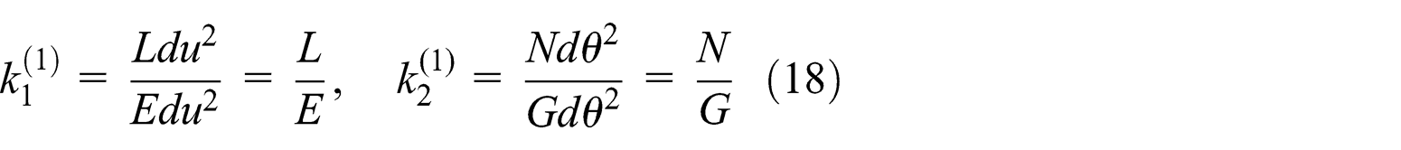
In general, $Ψ$ is called the curvature interference limit function or the limit function of the first kind.^13,21 Equation (12) can be regarded as a universal singular point condition for the generated tooth surface.

Elicitation of normal vector of instantaneous contact line

Equation (13) shows that the vector $\vec{N}$ is a linear combination of ${\vec{r}}_{1 u}$ and ${\vec{r}}_{1 θ}$ , so that it lies in the common tangential plane of $Σ_{1}$ and $Σ_{2}$ at an instantaneous meshing point. From equations (5) and (13), it is undemanding to know

{\vec{r}}_{1 u} • \vec{N} = - Φ_{u}, {\vec{r}}_{1 θ} • \vec{N} = - Φ_{θ}

(14)

When $φ = φ_{t} = const$ , on $Σ_{1}$ , the equation of the instantaneous contact line $L_{t}$ can be written as

{\vec{r}}_{1}^{(t)} = {\vec{r}}_{1} (u, θ), Φ (u, θ, φ_{t}) = 0

(15)

Therefore, the tangential vector of the instantaneous contact line $L_{t}$ can be figured out as

d_{1} {\vec{r}}_{1}^{(t)} = {\vec{r}}_{1 u} du + {\vec{r}}_{1 θ} d θ, Φ_{u} du + Φ_{θ} d θ = 0

(16)

Thereupon, it is possible to have $\vec{N} • d_{1} {\vec{r}}_{1}^{(t)} = 0$ . Hence, $\vec{N} ⊥ d_{1} {\vec{r}}_{1}^{(t)}$ and the vector $\vec{N}$ may be called the normal vector of the instantaneous contact line.

Diverse expressions for normal vector of instantaneous contact line

In fact, equation (13) provides a way to calculate $\vec{N}$ , whose operation is completely implemented in a non-unit and non-orthogonal natural moving frame ${P; {\vec{r}}_{1 u}, {\vec{r}}_{1 θ}, {\vec{n}}_{1}}$ . This makes the calculating process relatively cumbersome. In consequence, it is necessary to explore other ways to compute $\vec{N}$ .

In principal coordinate frame

If the parametric curve net on $Σ_{1}$ is consisted of the curvature lines, at an arbitrary point $P$ in the meshing region, the principal frame ${P; {\vec{g}}_{1}, {\vec{g}}_{2}, {\vec{n}}_{1}}$ can be constructed, in which ${\vec{g}}_{1}$ and ${\vec{g}}_{2}$ are the unit vectors along the two principal directions of $Σ_{1}$ , respectively.

In this case, it is easy to obtain the following results from differential geometry³⁶

{\vec{r}}_{1 u} = \sqrt{E} {\vec{g}}_{1}, {\vec{r}}_{1 θ} = \sqrt{G} {\vec{g}}_{2}, F = 0, M = 0

(17)

where $M$ is one of the coefficients of the second fundamental form of $Σ_{1}$ and $M = {\vec{r}}_{1 u θ} • {\vec{n}}_{1} = - {\vec{r}}_{1 u} • {\vec{n}}_{1 θ} = - {\vec{r}}_{1 θ} • {\vec{n}}_{1 u}$ .

By definition and from equation (17), the two principal curvatures of $Σ_{1}$ can be figured out as

k_{1}^{(1)} = \frac{Ld u^{2}}{Ed u^{2}} = \frac{L}{E}, k_{2}^{(1)} = \frac{Nd θ^{2}}{Gd θ^{2}} = \frac{N}{G}

(18)

where $L$ and $N$ are the other two coefficients of the second fundamental form of $Σ_{1}$ , and $L = {\vec{r}}_{1 uu} • {\vec{n}}_{1} = - {\vec{r}}_{1 u} • {\vec{n}}_{1 u}$ and $N = {\vec{r}}_{1 θ θ} • {\vec{n}}_{1} = - {\vec{r}}_{1 θ} • {\vec{n}}_{1 θ}$ .

According to the Weingarten formula³⁶ and using equations (17) and (18), it may have

\begin{matrix} {\vec{n}}_{1 u} = \frac{(FM - GL) {\vec{r}}_{1 u} + (FL - EM) {\vec{r}}_{1 θ}}{D^{2}} = - k_{1}^{(1)} \sqrt{E} {\vec{g}}_{1} \\ {\vec{n}}_{1 θ} = \frac{(FN - GM) {\vec{r}}_{1 u} + (FM - EN) {\vec{r}}_{1 θ}}{D^{2}} = - k_{2}^{(1)} \sqrt{G} {\vec{g}}_{2} \end{matrix}

(19)

Substitution of equation (19) into equation (5) can yield

\begin{matrix} Φ_{u} = - k_{1}^{(1)} \sqrt{E} {\vec{g}}_{1} • {\vec{V}}_{12} - \sqrt{E} {\vec{ω}}_{12} • [({\vec{g}}_{1} \times {\vec{g}}_{2}) \times {\vec{g}}_{1}] \\ = - \sqrt{E} (k_{1}^{(1)} {\vec{V}}_{12} • {\vec{g}}_{1} + {\vec{ω}}_{12} • {\vec{g}}_{2}) \\ Φ_{θ} = - k_{2}^{(1)} \sqrt{G} {\vec{g}}_{2} • {\vec{V}}_{12} - \sqrt{G} {\vec{ω}}_{12} • [({\vec{g}}_{1} \times {\vec{g}}_{2}) \times {\vec{g}}_{2}] \\ = - \sqrt{G} (k_{2}^{(1)} {\vec{V}}_{12} • {\vec{g}}_{2} - {\vec{ω}}_{12} • {\vec{g}}_{1}) \end{matrix}

(20)

Substituting equations (17) and (20) into equation (13) causes

\vec{N} = - \frac{Φ_{u}}{\sqrt{E}} {\vec{g}}_{1} - \frac{Φ_{θ}}{\sqrt{G}} {\vec{g}}_{2} = λ {\vec{g}}_{1} + μ {\vec{g}}_{2}

(21)

where $λ = k_{1}^{(1)} {\vec{V}}_{12} • {\vec{g}}_{1} + {\vec{ω}}_{12} • {\vec{g}}_{2} = - \frac{Φ_{u}}{\sqrt{E}}$ and $μ = k_{2}^{(1)} {\vec{V}}_{12} • {\vec{g}}_{2} - {\vec{ω}}_{12} • {\vec{g}}_{1} = - \frac{Φ_{θ}}{\sqrt{G}}$ .

If the two principal directions of $Σ_{1}$ are facile to be obtained, it is convenient to calculate $\vec{N}$ from equation (21). For example, the generating surface $Σ_{1}$ is a surface of revolution or an involute helicoidal surface. Otherwise, the calculation of $\vec{N}$ from equation (21) may still be rather tedious.

In arbitrary unit orthogonal frame

In reality, at a discretionary meshing point $P$ in the conjugate region of $Σ_{1}$ , a unit orthogonal moving frame, $σ_{P} {P; {\vec{α}}_{ξ}, {\vec{α}}_{η}, {\vec{n}}_{1}}$ , can be built freely. The second unit vector, ${\vec{α}}_{η}$ , can be determined as ${\vec{α}}_{η} = {\vec{n}}_{1} \times {\vec{α}}_{ξ}$ . The mere condition to select the first unit vector, ${\vec{α}}_{ξ}$ , is that the normal curvature and the geodesic torsion of $Σ_{1}$ along it are all easier to be achieved.

At the meshing point $P$ , the position relation between the principal frame and $σ_{P}$ is shown in Figure 2. By means of the circle vector function,³⁷ the representations of the two principal directions in $σ_{P}$ are

\begin{array}{l} {\vec{g}}_{1} = {\vec{e}}_{α} (- β) = \cos β \vec{α_{ξ}} - \sin β \vec{α_{η}}, \\ {\vec{g}}_{2} = {\vec{g}}_{α} (- β) = \sin β \vec{α_{ξ}} + \cos β \vec{α_{η}} \end{array}

(22)

where $β$ is a directed angle as depicted in Figure 2.

Figure 2.

Coordinate frames at instantaneous meshing point $P$ .

After substituting equation (22) into equation (21), the expression of the normal vector $\vec{N}$ in $σ_{P}$ can be worked out as

\begin{array}{l} \vec{N} = λ (\cos β \vec{α_{ξ}} - \sin β \vec{α_{η}}) + μ (\sin β \vec{α_{ξ}} + \cos β \vec{α_{η}}) \\ = N_{ξ} \vec{α_{ξ}} + N_{η} \vec{α_{η}} \end{array}

(23)

Based on the expressions of $λ$ and $μ$ in equation (21), by employing the Euler and Bertrand formulae in differential geometry,³⁶ the component of the normal vector $\vec{N}$ along the direction ${\vec{α}}_{ξ}$ can be worked out as below

\begin{matrix} N_{ξ} = λ \cos β + μ \sin β = {\vec{V}}_{12} • (k_{1} \cos β {\vec{g}}_{1} + k_{2} \sin β {\vec{g}}_{2}) + • {\vec{ω}}_{12} (\cos β {\vec{g}}_{2} - \sin β {\vec{g}}_{1}) \\ = {\vec{V}}_{12} • [k_{1} \cos β (\cos β {\vec{α}}_{ξ} - \sin β {\vec{α}}_{η}) + k_{2} \sin β (\sin β {\vec{α}}_{ξ} + \cos β {\vec{α}}_{η})] \\ + {\vec{ω}}_{12} • [- \sin β (\cos β {\vec{α}}_{ξ} - \sin β {\vec{α}}_{η}) + \cos β (\sin β {\vec{α}}_{ξ} + \cos β {\vec{α}}_{η})] \\ = {\vec{V}}_{12} • [(k_{1} \cos^{2} β + k_{2} \sin^{2} β) {\vec{α}}_{ξ} + (k_{2} - k_{1}) \sin β \cos β {\vec{α}}_{η}] + {\vec{ω}}_{12} • {\vec{α}}_{η} \\ = k_{ξ}^{(1)} {\vec{V}}_{12} • {\vec{α}}_{ξ} + τ_{ξ}^{(1)} {\vec{V}}_{12} • {\vec{α}}_{η} + {\vec{ω}}_{12} • {\vec{α}}_{η} \end{matrix}

(24)

where $k_{ξ}^{(1)}$ and $τ_{ξ}^{(1)}$ are the normal curvature and the geodesic torsion of the generating surface $Σ_{1}$ along the direction ${\vec{α}}_{ξ}$ in several.

In the same manner, the component of the normal vector $\vec{N}$ along the direction ${\vec{α}}_{η}$ can be ciphered out as follows

N_{η} = τ_{ξ}^{(1)} {\vec{V}}_{12} • {\vec{α}}_{ξ} + k_{η}^{(1)} {\vec{V}}_{12} • {\vec{α}}_{η} - {\vec{ω}}_{12} • {\vec{α}}_{ξ}

(25)

where $k_{η}^{(1)}$ is the normal curvature of $Σ_{1}$ along the direction ${\vec{α}}_{η}$ and can be figured down as $k_{η}^{(1)} = 2 H^{(1)} - k_{ξ}^{(1)}$ , in which $H^{(1)}$ is the mean curvature of $Σ_{1}$ .³⁸

In nature, equation (21) can be regarded as a special circumstance of equation (23) because when ${\vec{α}}_{ξ} = {\vec{g}}_{1}$ and ${\vec{α}}_{η} = {\vec{g}}_{2}$ , $k_{ξ}^{(1)} = k_{1}^{(1)}$ , $k_{η}^{(1)} = k_{2}^{(1)}$ , and $τ_{ξ}^{(1)} = 0$ and equation (23) degenerates into equation (21). Thus, equation (23) can be seen as the universal approach to calculate $\vec{N}$ .

Provided the principal directions of the generating surface $Σ_{1}$ are difficult to be acquired, it is recommended to calculate $\vec{N}$ by right of equation (23). For instance, the generating surface $Σ_{1}$ is the helicoidal surface of a ZN worm or a Hindley worm.

In velocity coordinate frame

Letting ${\vec{α}}_{ξ} = {\vec{V}}_{12} / | {\vec{V}}_{12} |$ causes ${\vec{α}}_{η} = ({\vec{n}}_{1} \times {\vec{V}}_{12}) / | {\vec{V}}_{12} |$ and a velocity coordinate frame can be attained. From equation (23), the expression of $\vec{N}$ in such a velocity coordinate frame can be represented as

\vec{N} = {\vec{ω}}_{12} \times {\vec{n}}_{1} + k_{v}^{(1)} {\vec{V}}_{12} + τ_{v}^{(1)} {\vec{n}}_{1} \times {\vec{V}}_{12}

(26)

where $k_{v}^{(1)}$ and $τ_{v}^{(1)}$ are the normal curvature and the geodesic torsion of $Σ_{1}$ along ${\vec{V}}_{12}$ in several.

Representation based on derivative of unit normal vector

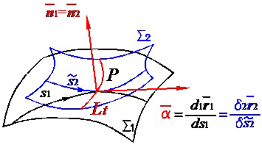
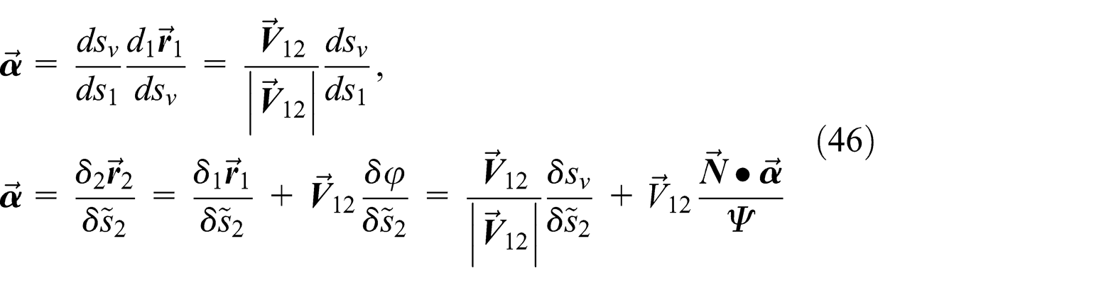
According to the result in differential geometry,³⁶ along the direction of the relative velocity vector ${\vec{V}}_{12}$ on $Σ_{1}$ , the derivative of ${\vec{n}}_{1}$ can be expressed as

\frac{d_{1} {\vec{n}}_{1}}{d s_{v}} = - k_{v}^{(1)} \frac{{\vec{V}}_{12}}{| {\vec{V}}_{12} |} - τ_{v}^{(1)} \frac{{\vec{n}}_{1} \times {\vec{V}}_{12}}{| {\vec{V}}_{12} |}

(27)

where $s_{v}$ is the arc length of a curve on $Σ_{1}$ , whose tangential direction at the instantaneous meshing point $P$ is along the velocity vector ${\vec{V}}_{12}$ , as shown in Figure 1.

From equations (26) and (27), it is possible to have

\vec{N} = {\vec{ω}}_{12} \times {\vec{n}}_{1} - | {\vec{V}}_{12} | \frac{d_{1} {\vec{n}}_{1}}{d s_{v}}

(28)

Induced normal curvature of line-conjugate surface couple

Preparative relation expressions

As shown in Figure 3, the symbol $\vec{α}$ denotes a unit common tangential vector of both $Σ_{1}$ and $Σ_{2}$ . At the same time, the notations $s_{1}$ and ${\tilde{s}}_{2}$ are the arc lengths of the curves separately on $Σ_{1}$ and $Σ_{2}$ , whose unit tangential vectors are all $\vec{α}$ . Consequently, it is easy to have

\vec{α} = \frac{d_{1} {\vec{r}}_{1}}{d s_{1}} = \frac{δ_{2} {\vec{r}}_{2}}{δ {\tilde{s}}_{2}}

(29)

Figure 3.

Unit common tangential vector $\vec{α}$ and arc lengths $s_{1}$ and ${\tilde{s}}_{2}$ .

Accomplishing the dot product regarding $\vec{N}$ on both sides of equation (29) and making use of the relative differential method give

\vec{N} • \frac{δ_{1} {\vec{r}}_{1}}{δ {\tilde{s}}_{2}} = \vec{N} • \vec{α} - \vec{N} • {\vec{V}}_{12} \frac{δ φ}{δ {\tilde{s}}_{2}}

(30)

On account of ${\vec{V}}_{12} = | {\vec{V}}_{12} | \frac{d_{1} {\vec{r}}_{1}}{d s_{v}} = | {\vec{V}}_{12} | \frac{δ_{1} {\vec{r}}_{1}}{δ s_{v}}$ , from equations (7), (28), and (29), it is possible to have

\begin{matrix} Φ_{φ} \frac{d φ}{d s_{1}} = ({\vec{ω}}_{12}, {\vec{n}}_{1}, \frac{d_{1} {\vec{r}}_{1}}{d s_{1}}) - \frac{d_{1} {\vec{n}}_{1}}{d s_{1}} • \\ {\vec{V}}_{12} = ({\vec{ω}}_{12}, {\vec{n}}_{1}, \frac{d_{1} {\vec{r}}_{1}}{d s_{1}}) - | {\vec{V}}_{12} | \frac{d_{1} {\vec{n}}_{1}}{d s_{v}} • \frac{d_{1} {\vec{r}}_{1}}{d s_{1}} \\ = \vec{α} • ({\vec{ω}}_{12} \times {\vec{n}}_{1} - | {\vec{V}}_{12} | \frac{d_{1} {\vec{n}}_{1}}{d s_{v}}) = \vec{α} • \vec{N} \end{matrix}

(31)

Likewise, from equations (7) and (28), it may have

\begin{array}{l} Φ_{φ} \frac{δ φ}{δ {\tilde{s}}_{2}} = (\vec{ω_{12}}, {\vec{n}}_{1}, \frac{δ_{1} {\vec{r}}_{1}}{δ {\tilde{s}}_{2}}) - \frac{δ_{1} {\vec{n}}_{1}}{δ {\tilde{s}}_{2}} • {\vec{V}}_{12} \\ = (\vec{ω_{12}}, {\vec{n}}_{1}, \frac{δ_{1} {\vec{r}}_{1}}{δ {\tilde{s}}_{2}}) - | {\vec{V}}_{12} | \frac{δ_{1} {\vec{n}}_{1}}{δ {\tilde{s}}_{2}} • \frac{δ_{1} {\vec{r}}_{1}}{δ s_{v}} = \vec{N} • \frac{δ_{1} {\vec{r}}_{1}}{δ {\tilde{s}}_{2}} \end{array}

(32)

From equations (30) and (32), $δ φ / δ {\tilde{s}}_{2}$ can be figured down. Simplifying the obtained result by means of equations (12), (28), and (31) yields

\begin{array}{l} \frac{δ φ}{δ {\tilde{s}}_{2}} = \frac{\vec{N} • \vec{α}}{Ψ} = \frac{Φ_{φ}}{Ψ} \frac{d φ}{d s_{1}} \\ = \frac{1}{Ψ} [(\vec{ω_{12}}, {\vec{n}}_{1}, \frac{d_{1} {\vec{r}}_{1}}{d s_{1}}) - \frac{d_{1} {\vec{n}}_{1}}{d s_{1}} • {\vec{V}}_{12}] \end{array}

(33)

Straightforwardly, it is uncomplicated to prove the following commutation relation with regard to the relative differential signs as

\begin{array}{l} d_{1} {\vec{r}}_{1} • δ_{1} {\vec{n}}_{1} = - L d u δ u - M (d u δ θ + d θ δ u) \\ - N d θ δ θ = δ_{1} {\vec{r}}_{1} • d_{1} {\vec{n}}_{1} \end{array}

(34)

Deducing process of induced normal curvature formula

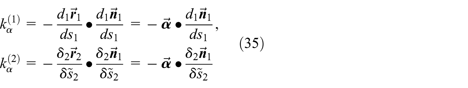
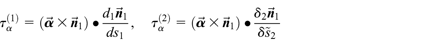
By definition, the normal curvatures of $Σ_{1}$ and $Σ_{2}$ along $\vec{α}$ can be represented as

\begin{array}{l} k_{α}^{(1)} = - \frac{d_{1} {\vec{r}}_{1}}{d s_{1}} • \frac{d_{1} {\vec{n}}_{1}}{d s_{1}} = - \vec{α} • \frac{d_{1} {\vec{n}}_{1}}{d s_{1}}, \\ k_{α}^{(2)} = - \frac{δ_{2} {\vec{r}}_{2}}{δ {\tilde{s}}_{2}} • \frac{δ_{2} {\vec{n}}_{1}}{δ {\tilde{s}}_{2}} = - \vec{α} • \frac{δ_{2} {\vec{n}}_{1}}{δ {\tilde{s}}_{2}} \end{array}

(35)

Thereupon, the induced normal curvature of the line-conjugate surface couple $[Σ_{1}, Σ_{2}]$ along $\vec{α}$ can be defined as $k_{α}^{(12)} = k_{α}^{(1)} - k_{α}^{(2)}$ . After substituting equation (35) into the preceding definition expression and reducing the attained result in terms of the relative differential method and using equations (28) and (29), it maybe has

\begin{matrix} k_{α}^{(12)} = k_{α}^{(1)} - k_{α}^{(2)} = k_{α}^{(1)} + \frac{d_{1} {\vec{r}}_{1}}{d s_{1}} • (\frac{δ_{1} {\vec{n}}_{1}}{δ {\tilde{s}}_{2}} + {\vec{ω}}_{12} \times {\vec{n}}_{1} \frac{δ φ}{δ {\tilde{s}}_{2}}) \\ = k_{α}^{(1)} + \frac{d_{1} {\vec{n}}_{1}}{d s_{1}} • \frac{δ_{1} {\vec{r}}_{1}}{δ {\tilde{s}}_{2}} + ({\vec{ω}}_{12}, {\vec{n}}_{1}, \frac{d_{1} {\vec{r}}_{1}}{d s_{1}}) \frac{δ φ}{δ {\tilde{s}}_{2}} \\ = k_{α}^{(1)} + \frac{d_{1} {\vec{n}}_{1}}{d s_{1}} • (\frac{δ_{2} {\vec{r}}_{2}}{δ {\tilde{s}}_{2}} - {\vec{V}}_{12} \frac{δ φ}{δ {\tilde{s}}_{2}}) \\ + ({\vec{ω}}_{12}, {\vec{n}}_{1}, \frac{d_{1} {\vec{r}}_{1}}{d s_{1}}) \frac{δ φ}{δ {\tilde{s}}_{2}} \\ = [({\vec{ω}}_{12}, {\vec{n}}_{1}, \frac{d_{1} {\vec{r}}_{1}}{d s_{1}}) - \frac{d_{1} {\vec{n}}_{1}}{d s_{1}} • {\vec{V}}_{12}] \frac{δ φ}{δ {\tilde{s}}_{2}} \end{matrix}

(36)

According to equation (33), equation (36) can be transformed into

k_{α}^{(12)} = \frac{1}{Ψ} {[({\vec{ω}}_{12}, {\vec{n}}_{1}, \frac{d_{1} {\vec{r}}_{1}}{d s_{1}}) - \frac{d_{1} {\vec{n}}_{1}}{d s_{1}} • {\vec{V}}_{12}]}^{2}

(37a)

= \frac{1}{Ψ} {(Φ_{φ} \frac{d φ}{d s_{1}})}^{2}

(37b)

= \frac{{(\vec{α} • \vec{N})}^{2}}{Ψ}

(37c)

Actually, both equations (37a) and (37b) are not suitable for being used to compute the induced normal curvature and can only be viewed as the middle results in the process of deducing the induced normal curvature formula. The reason is that $d_{1} {\vec{n}}_{1} / d s_{1}$ and $d φ / d s_{1}$ have to be worked out in advance. Furthermore, the related computation is lack of the distinct geometrical significance. Consequently, the user-friendly formula for the induced normal curvature should be equation (37c).

Affiliated outcomes

Letting $\vec{α} = {\vec{V}}_{12} / | {\vec{V}}_{12} |$ in equation (37c) and using equation (12) to simplify the consequence, the induced normal curvature along ${\vec{V}}_{12}$ can compactly be obtained as

k_{v}^{(12)} = \frac{{(Ψ - Φ_{φ})}^{2}}{Ψ {| {\vec{V}}_{12} |}^{2}}

(38)

Without loss of generality, choosing the frame $σ_{P}$ to express the vector $\vec{α}$ yields

\vec{α} = \cos ϕ {\vec{α}}_{ξ} + \sin ϕ {\vec{α}}_{η}

(39)

where $ϕ$ is a directed angle as illustrated in Figure 4.

Figure 4.

Induced principal directions and unit common tangential vector $\vec{α}$ .

Substituting equations (23) and (39) into equation (37c) leads up to

k_{α}^{(12)} = \frac{1}{Ψ} {(N_{ξ} \cos ϕ + N_{η} \sin ϕ)}^{2}

(40)

Equation (40) is the computing formula for the induced normal curvature in the scalar form, which is equivalent to equation (37c).

After knowing the induced normal curvature, the homologous normal curvature of the generated surface $Σ_{2}$ can be acquired without differentiating its equation.

Induced geodesic torsion and induced principal directions

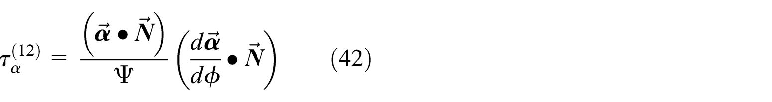
Induced geodesic torsion formula

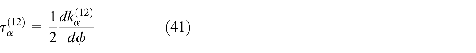
There are two strategies to deduce the computing formula for the induced geodesic torsion. One strategy is to begin with the induced normal curvature. According to their definitions, the induced normal curvature, $k_{α}^{(12)}$ , and the induced geodesic torsion, $τ_{α}^{(12)}$ , still are the normal curvature and the geodesic torsion in essence. In consequence, the derivative relation is in existence between them, namely

τ_{α}^{(12)} = \frac{1}{2} \frac{{dk}_{α}^{(12)}}{d ϕ}

(41)

Since both $\vec{N}$ and $Ψ$ are all constant at a certain meshing point, substituting equation (37) into (41) causes

τ_{α}^{(12)} = \frac{(\vec{α} • \vec{N})}{Ψ} (\frac{d \vec{α}}{d ϕ} • \vec{N})

(42)

Owing to $| \vec{α} | = 1$ , $(d \vec{α} / d ϕ) ⊥ \vec{α}$ . Since at a certain meshing point ${\vec{n}}_{1}$ is not concerned with the angle $ϕ$ and $\vec{α} • {\vec{n}}_{1} = 0$ , $(d \vec{α} / d ϕ) ⊥ {\vec{n}}_{1}$ . As a result, in order to guarantee that the frame ${P; \vec{α}, d \vec{α} / d ϕ, {\vec{n}}_{1}}$ is right-handed, $d \vec{α} / d ϕ$ can be represented as

\frac{d \vec{α}}{d ϕ} = | \frac{d \vec{α}}{d ϕ} | {\vec{n}}_{1} \times \vec{α}

(43)

Because the two base vectors ${\vec{α}}_{ξ}$ and ${\vec{α}}_{η}$ all have nothing to do with the angle $ϕ$ at a certain meshing point, it is uncomplicated to understand $| \frac{d \vec{α}}{d ϕ} | = 1$ from equation (39). Substituting this outcome into equation (43) leads to $(d \vec{α} / d ϕ) = {\vec{n}}_{1} \times \vec{α}$ . After substituting this outcome into equation (42), the computing formula for $τ_{α}^{(12)}$ in the vector form can be attained as

τ_{α}^{(12)} = \frac{1}{Ψ} (\vec{α} • \vec{N}) (\vec{α}, \vec{N}, {\vec{n}}_{1})

(44)

The other strategy to deduce the computing formula for the induced geodesic torsion is to begin with the definition thoroughly. The geodesic torsions of $Σ_{1}$ and $Σ_{2}$ along the common tangential direction $\vec{α}$ can be represented as

τ_{α}^{(1)} = (\vec{α} \times {\vec{n}}_{1}) • \frac{d_{1} {\vec{n}}_{1}}{d s_{1}}, τ_{α}^{(2)} = (\vec{α} \times {\vec{n}}_{1}) • \frac{δ_{2} {\vec{n}}_{1}}{δ {\tilde{s}}_{2}}

By definition and with the help of equations (4), (28), and (33), the induced geodesic torsion, $τ_{α}^{(12)}$ , can thus be procured as

\begin{matrix} τ_{α}^{(12)} = τ_{α}^{(1)} - τ_{α}^{(2)} = (\vec{α} \times {\vec{n}}_{1}) • (\frac{d_{1} {\vec{n}}_{1}}{d s_{1}} - \frac{δ_{2} {\vec{n}}_{1}}{δ {\tilde{s}}_{2}}) • \\ = (\vec{α} \times {\vec{n}}_{1}) (\frac{d_{1} {\vec{n}}_{1}}{d s_{1}} - \frac{δ_{1} {\vec{n}}_{1}}{δ {\tilde{s}}_{2}} - {\vec{ω}}_{12} \times {\vec{n}}_{1} \frac{δ φ}{δ {\tilde{s}}_{2}}) \\ = (\vec{α} \times {\vec{n}}_{1}) • [(\frac{d s_{v}}{d s_{1}} - \frac{δ s_{v}}{δ {\tilde{s}}_{2}}) \frac{{\vec{ω}}_{12} \times {\vec{n}}_{1} - \vec{N}}{| {\vec{V}}_{12} |} - \frac{\vec{N} \vec{•} α}{Ψ} {\vec{ω}}_{12} \times {\vec{n}}_{1}] \end{matrix}

(45)

From equation (29), it may have

\begin{array}{l} \vec{α} = \frac{d s_{v}}{d s_{1}} \frac{d_{1} {\vec{r}}_{1}}{d s_{v}} = \frac{{\vec{V}}_{12}}{| {\vec{V}}_{12} |} \frac{d s_{v}}{d s_{1}}, \vec{α} = \frac{δ_{2} {\vec{r}}_{2}}{δ {\tilde{s}}_{2}} \\ = \frac{δ_{1} {\vec{r}}_{1}}{δ {\tilde{s}}_{2}} + {\vec{V}}_{12} \frac{δ φ}{δ {\tilde{s}}_{2}} = \frac{{\vec{V}}_{12}}{| {\vec{V}}_{12} |} \frac{δ s_{v}}{δ {\tilde{s}}_{2}} + {\vec{V}}_{12} \frac{\vec{N} • \vec{α}}{Ψ} \end{array}

(46)

Executing the dot products on the both sides of the two expressions in equation (46) in regard of $\vec{N}$ , respectively, leads up to

\frac{d s_{v}}{d s_{1}} = | {\vec{V}}_{12} | \frac{\vec{N} • \vec{α}}{\vec{N} • {\vec{V}}_{12}}, \frac{δ s_{v}}{δ {\tilde{s}}_{2}} = | {\vec{V}}_{12} | \frac{Φ_{φ}}{Ψ} \frac{\vec{N} • \vec{α}}{\vec{N} • {\vec{V}}_{12}}

(47)

Substitution of equation (47) into equation (45), after simplification, brings about equation (44). Substituting equations (23) and (39) into equation (44) can yield the formula to compute $τ_{α}^{(12)}$ in the scalar form as

τ_{α}^{(12)} = \frac{- 1}{Ψ} (N_{ξ} \cos ϕ + N_{η} \sin ϕ) (N_{ξ} \sin ϕ - N_{η} \cos ϕ)

(48)

Induced principal directions and induced principal curvatures

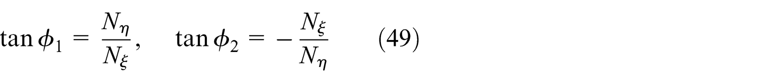
Because there is the derivative relation between the induced normal curvature and the induced geodesic torsion as depicted in equation (41), the induced normal curvature have its maximum value along the direction along which $τ_{α}^{(12)} = 0$ . That is to say, such a direction is the induced principal direction. By letting $τ_{α}^{(12)} = 0$ in equation (48), two directed angles, $ϕ_{1}$ and $ϕ_{2}$ , can be worked out over the interval $[0, π]$ , which can be employed to determine the two induced principal directions in the unit orthogonal moving frame $σ_{P} {P; {\vec{α}}_{ξ}, {\vec{α}}_{η}, {\vec{n}}_{1}}$ . The tangent values of these two directed angles are

\tan ϕ_{1} = \frac{N_{η}}{N_{ξ}}, \tan ϕ_{2} = - \frac{N_{ξ}}{N_{η}}

(49)

From equation (49), it may have $\tan ϕ_{2} = \tan (ϕ_{1} + 90 \circ)$ . One solution of this trigonometric equation with respect to $ϕ_{2}$ is $ϕ_{2} = ϕ_{1} + 90 \circ$ . Hence, the two induced principal directions are perpendicular to each other. Additionally, equation (49) illustrates that one induced principal direction is along the normal direction of the instantaneous contact line so that the other is along its tangential direction.

Letting ${\vec{α}}_{t}$ denote the unit tangential vector along the instantaneous contact line, under the condition that the moving frame ${P; \vec{N}, {\vec{α}}_{t}, {\vec{n}}_{1}}$ is right-handed, ${\vec{α}}_{t}$ can be expressed as

{\vec{α}}_{t} = \frac{{\vec{n}}_{1} \times \vec{N}}{| \vec{N} |} = \frac{- N_{η} {\vec{α}}_{ξ} + N_{ξ} {\vec{α}}_{η}}{\sqrt{N_{ξ}^{2} + N_{η}^{2}}}

(50)

By substituting equations (23) and (50) into equation (37), respectively, the two induced principal curvatures along the two induced principal directions can be worked out as

k_{t}^{(12)} = 0, k_{N}^{(12)} = \frac{{| \vec{N} |}^{2}}{Ψ}

(51)

Equation (51) manifests that the non-zero induced principal curvature is along the normal direction of the momentary contact line and the zero induced principal curvature is along its tangential direction. Hence, the maximum absolute value of $k_{α}^{(12)}$ takes place along the direction $\vec{N}$ .

In the bargain, the induced Gauss curvature of the line-conjugate tooth surface couple can be obtained as $K^{(12)} = k_{t}^{(12)} k_{N}^{(12)} = 0$ . Consequently, the regular meshing points of a line-conjugate tooth surface couple are all the induced parabolic points.

Because ${| \vec{N} |}^{2}$ can be ciphered out from equations (13), (21), and (23), the computing formula in the scalar form for $k_{N}^{(12)}$ will have the related manifestation, which is listed as follows

k_{N}^{(12)} = \frac{1}{D^{2} Ψ} (G Φ_{u}^{2} - 2 F Φ_{u} Φ_{θ} + E Φ_{θ}^{2}), {P; {\vec{r}}_{1 u}, {\vec{r}}_{1 θ}, {\vec{n}}_{1}}

(52)

= \frac{λ^{2} + μ^{2}}{Ψ}, {P; {\vec{g}}_{1}, {\vec{g}}_{2}, {\vec{n}}_{1}}

(53)

= \frac{N_{ξ}^{2} + N_{η}^{2}}{Ψ}, {P; {\vec{α}}_{ξ}, {\vec{α}}_{η}, {\vec{n}}_{1}}

(54)

In principle, it is not recommended to compute $k_{N}^{(12)}$ by means of equation (52). The reason is that the partial derivatives of the meshing function have to be calculated on the side after acquiring $Ψ$ from equation (12) based on the normal vector of the instantaneous contact line, $\vec{N}$ . If the two principal directions of the generating surface are simple to be worked out, equation (53) is proposed to be employed and otherwise equation (54) is proposed to be employed.

From equation (53) or (54), the sign of $k_{N}^{(12)}$ depends on that of $Ψ$ . The point on $Σ_{2}$ where $Ψ = 0$ is its singular point. So, in a practical meshing analysis, if the sign of $k_{N}^{(12)}$ changes in the whole conjugate zone, it can be concluded that the undercutting exists on the tooth surface of the gear 2.

When evaluating the contact stress for a line-conjugate tooth surface couple, the contact between its tooth surfaces is usually boiled down to the contact of two elastic cylinders owing to the complexity of the geometry. The two cylinders have the parallel axial lines and are in contact along the straight generatrix, which can circa be viewed as the instantaneous contact line of the surface couple. In line with the Hertz formula in the elastic contact mechanics,^3,4 the maximum pressure between the teeth can be calculated as

σ_{H} = Z_{E} \sqrt{W_{n} k_{N}^{(12)}}

(55)

where $Z_{E}$ is a material constant and $W_{n}$ is the normal force per unit length along the instantaneous contact line of the tooth surface couple.

In the matter of the tooth surface couple under consideration, the parameter $Z_{E}$ is constant and the parameter $W_{n}$ is almost constant during the action of the tooth surface couple. Therefore, equation (55) implies that the contact stress level, namely the value of $σ_{H}$ , approximately is proportional to $\sqrt{k_{N}^{(12)}}$ at a meshing point. This is the reason why the induced principal curvature can be adopted to reveal the contact stress level between the teeth in the rough. This also is one of the significant intentions to compute the induced principal curvature.

Induced curvature parameter computation for modified Hindley worm drive

Equation of worm helicoid and its unit normal vector

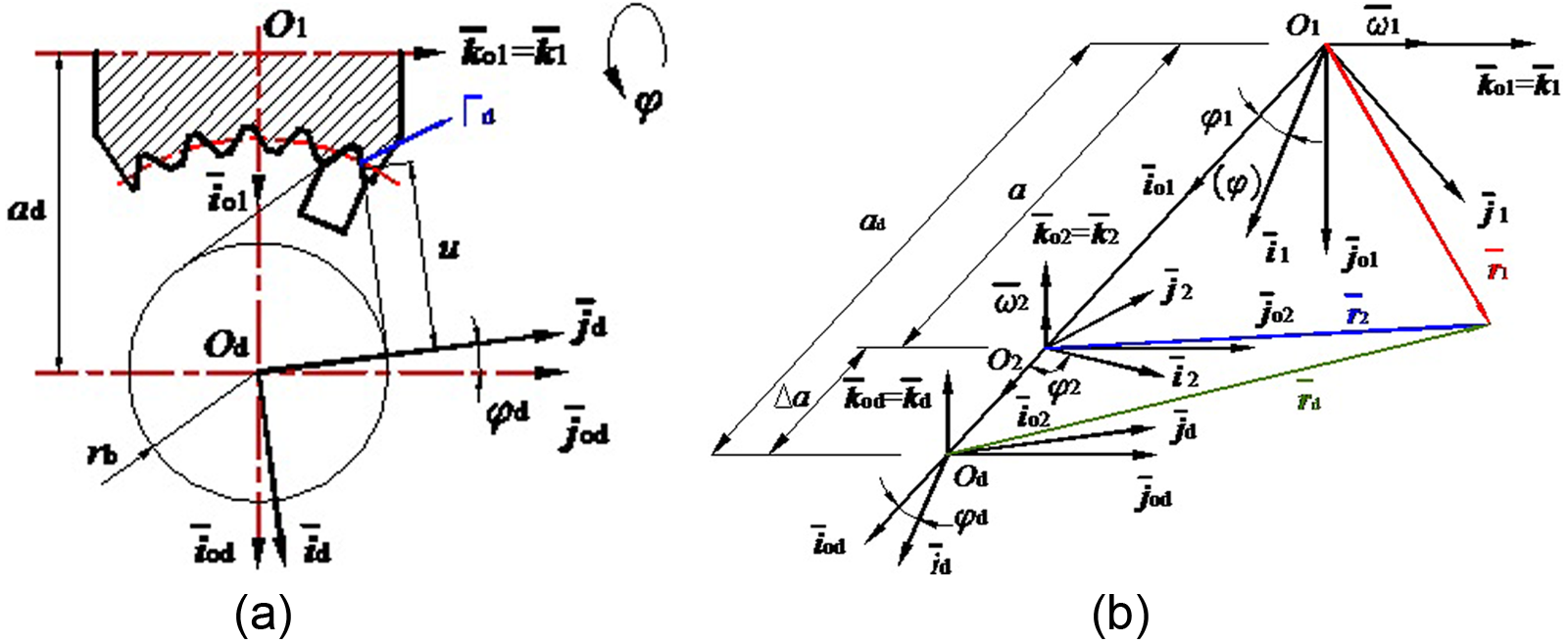
As illustrated in Figure 5, by right of the machining principle of the Hindley worm drive, two fixed coordinate systems, $σ_{o 1} {O_{1}; {\vec{i}}_{o 1}, {\vec{j}}_{o 1}, {\vec{k}}_{o 1}}$ and $σ_{od} {O_{d}; {\vec{i}}_{od}, {\vec{j}}_{od}, {\vec{k}}_{od}}$ , are used to indicate the initial positions of the worm blank and the tool post, respectively. Herein the two unit vectors, ${\vec{k}}_{o 1}$ and ${\vec{k}}_{od}$ , lie separately along their axial lines. Such two unit vectors are mutually perpendicular and the shortest distance between them is the distance from the point $O_{d}$ to $O_{1}$ , and $| \vec{O_{1} O_{d}} | = a_{d}$ . Therein $a_{d}$ is the operating center distance for machining the modified worm and $a_{d} = a + Δ a$ , where $a$ is the center distance of the worm pair and $Δ a$ is the modification quantity of the center distance.

Figure 5.

Formation mechanism of modified Hindley worm pair: (a) schematic diagram for machining modified Hindley worm and (b) position relation among coordinate systems.

Over and above that, two rotatable coordinate systems, $σ_{1}$ and $σ_{d} {O_{d}; {\vec{i}}_{d}, {\vec{j}}_{d}, {\vec{k}}_{d}}$ , are linked to the worm roughcast and the cutter frame, respectively. When the rotation angle of the worm roughcast is $φ$ , the interconnected rotating angle of the tool apron is $φ_{d}$ and $φ_{d} = φ / i_{1 d}$ , in which $i_{1 d}$ is the operating transmission ratio for cutting the worm blank and $i_{1 d} = i_{12} + Δ i$ . Here, $i_{12}$ is the transmitting ratio of the worm drive and $Δ i$ is the modification quantity of the transmission ratio.

In this study, both $Δ a$ and $Δ i$ are constant. In $σ_{d}$ , the vector equation of the straight cutting edge, $Γ_{d}$ , can be represented as

{({\vec{r}}_{d})}_{d} = - u {\vec{i}}_{d} + r_{b} {\vec{j}}_{d}

(56)

where $r_{b}$ is the main basic circle radius of the worm gear.

Via the coordinate transformation, it is possible to attain the equation for the spiral surface, $Σ_{1}$ , of the modified Hindley worm in $σ_{1}$ , which can be expressed as

\begin{matrix} {({\vec{r}}_{1})}_{1} = R [{\vec{k}}_{1}, - φ] (R [{\vec{i}}_{o 1}, \frac{π}{2}] R [{\vec{k}}_{od}, φ_{d}] {({\vec{r}}_{d})}_{d} + a_{d} {\vec{i}}_{o 1}) \\ = (x_{od} + a_{d}) \cos φ {\vec{i}}_{1} - (x_{od} + a_{d}) \sin φ {\vec{j}}_{1} + y_{od} {\vec{k}}_{1} \\ = {\vec{r}}_{1} (u, φ) \end{matrix}

(57)

where $x_{od} = - u \cos φ_{d} - r_{b} \sin φ_{d}$ , $y_{od} = - u \sin φ_{d} + r_{b} \cos φ_{d}$ , and $u$ and $φ$ are the two parameters of $Σ_{1}$ . The symbols, $R [{\vec{k}}_{od}, φ_{d}]$ , $R [{\vec{i}}_{o 1}, π / 2]$ , and $R [{\vec{k}}_{1}, - φ]$ denote the rotation transformation matrices.^20,21

By reason of

\frac{\partial x_{od}}{\partial φ} = - \frac{y_{od}}{i_{1 d}}, \frac{\partial y_{od}}{\partial φ} = \frac{x_{od}}{i_{1 d}}

(58)

it is possible to have

{({\vec{r}}_{1 u})}_{1} = - \cos φ_{d} \cos φ {\vec{i}}_{1} + \cos φ_{d} \sin φ {\vec{j}}_{1} - \sin φ_{d} {\vec{k}}_{1}

(59)

\begin{array}{l} {({\vec{r}}_{1 φ})}_{1} = - [\frac{y_{od}}{i_{1 d}} \cos φ + (x_{od} + a_{d}) \sin φ] {\vec{i}}_{1} \\ + [\frac{y_{od}}{i_{1 d}} \sin φ - (x_{od} + a_{d}) \cos φ] {\vec{j}}_{1} + \frac{x_{od}}{i_{1 d}} {\vec{k}}_{1} \end{array}

(60)

From equations (59) and (60), the coefficients of the first fundamental form of $Σ_{1}$ can be acquired as follows

E = 1, F = \frac{r_{b}}{i_{1 d}}, G = {(x_{od} + a_{d})}^{2} + \frac{1}{i_{1 d}^{2}} (u^{2} + r_{b}^{2})

(61)

On the basis of equation (3), the unit normal vector of $Σ_{1}$ can be obtained as

{({\vec{n}}_{1})}_{1} = \frac{{({\vec{r}}_{1 u})}_{1} \times {({\vec{r}}_{1 φ})}_{1}}{D} = n_{1 x} {\vec{i}}_{1} + n_{1 y} {\vec{j}}_{1} + n_{1 z} {\vec{k}}_{1}

(62)

where $n_{1 x} = (- 1 / i_{1 d} D) [i_{1 d} (x_{od} + a_{d}) \sin φ_{d} \cos φ + u \sin φ]$ , $n_{1 y} = (1 / i_{1 d} D) [i_{1 d} (x_{od} + a_{d}) \sin φ_{d} \sin φ - u \cos φ]$ , $n_{1 z} = ((x_{od} + a_{d}) / D) \cos φ_{d}$ , and $D = \sqrt{{(x_{od} + a_{d})}^{2} + (u^{2} / i_{1 d}^{2})}$ .

Curvature parameters of worm helicoid and moving frame on it

Due to $F \neq 0$ for $Σ_{1}$ as shown by equation (61), its parameter curve net is not made up of the curvature lines. In such a case, it is suitable for selecting equation (23), instead of equation (21), to calculate $\vec{N}$ in terms of the analysis in section “In arbitrary unit orthogonal frame.” For this, it is profitable to let the unit vector ${\vec{α}}_{ξ}$ be along the tangential orientation of the parameter u-line of $Σ_{1}$ , namely

\begin{array}{l} {(\vec{α_{ξ}})}_{1} = \frac{{({\vec{r}}_{1 u})}_{1}}{| {({\vec{r}}_{1 u})}_{1} |} = - \cos φ_{d} \cos φ {\vec{i}}_{1} \\ + \cos φ_{d} \sin φ {\vec{j}}_{1} - \sin φ_{d} {\vec{k}}_{1} \end{array}

(63)

so that

{({\vec{α}}_{η})}_{1} = {({\vec{n}}_{1})}_{1} \times {({\vec{α}}_{ξ})}_{1} = α_{η x} {\vec{i}}_{1} + α_{η y} {\vec{j}}_{1} + α_{η z} {\vec{k}}_{1}

(64)

where

α_{η x} = \frac{- 1}{i_{1 d} D} [i_{1 d} (x_{od} + a_{d}) \sin φ - u \sin φ_{d} \cos φ]

α_{η y} = \frac{- 1}{i_{1 d} D} [i_{1 d} (x_{od} + a_{d}) \cos φ + u \sin φ_{d} \sin φ]

α_{η z} = - \frac{u}{i_{1 d} D} \cos φ_{d}

Concerning $Σ_{1}$ , the normal curvature and the geodesic torsion along ${\vec{α}}_{ξ}$ and its mean curvature can be achieved as³⁸

\begin{array}{l} k_{ξ}^{(1)} = 0, τ_{ξ}^{(1)} = - \frac{a_{d} - r_{b} \sin φ_{d}}{i_{1 d} D^{2}}, \\ H^{(1)} = - \frac{F τ_{ξ}^{(1)} - \sin φ_{d}}{2 D} - \frac{u}{2 i_{1 d}^{2} D^{3}} y_{od} \end{array}

(65)

Relative motion

During the engagement of the modified Hindley worm drive, also as shown in Figure 5, two fixed coordinate systems $σ_{o 1}$ and $σ_{o 2} {O_{2}; {\vec{i}}_{o 2}, {\vec{j}}_{o 2}, {\vec{k}}_{o 2}}$ are utilized to indicate the initial positions of the worm and the worm gear, respectively. Herein the two unit vectors, ${\vec{k}}_{o 1}$ and ${\vec{k}}_{o 2}$ , are separately along their axial lines and mutually perpendicular since the discussion in this work is limited to the worm pair with orthogonal axes. The shortest distance between the axes ${\vec{k}}_{o 1}$ and ${\vec{k}}_{o 2}$ is the distance from the point $O_{1}$ to $O_{2}$ , and $| \vec{O_{2} O_{1}} | = a$ .

In addition, two rotatable coordinate systems, $σ_{1}$ and $σ_{2}$ , are linked to the worm and the worm gear in several. When the rotation angle of the worm is $φ_{1}$ , the interconnected rotating angle of the worm gear is $φ_{2}$ and $φ_{2} = φ_{1} / i_{12}$ .

By the convention in section “Equation of generated tooth surface and partial derivatives of meshing function,” the worm rotates around ${\vec{k}}_{o 1}$ with the angle velocity $| {\vec{ω}}_{1} | = 1 rad / s$ and suitably the angle velocity of the worm gear is $| {\vec{ω}}_{2} | = (1 / i_{12}) rad / s$ . Ergo, the relative angle velocity vector of the worm pair can be figured out in $σ_{o 1}$ as

({\vec{ω}}_{12})_{o 1} = \frac{1}{i_{12}} {\vec{j}}_{o 1} + {\vec{k}}_{o 1}

(66)

By the definition stated in equation (3), the relative velocity vector of the worm pair can be obtained in $σ_{o 1}$ as

{({\vec{V}}_{12})}_{o 1} = (\frac{y_{od}}{i_{12}} - y_{o 1}) {\vec{i}}_{o 1} + x_{o 1} {\vec{j}}_{o 1} - \frac{x_{o 1} - a}{i_{12}} {\vec{k}}_{o 1}

(67)

where $x_{o 1} = (x_{od} + a_{d}) \cos (φ_{1} - φ)$ and $y_{o 1} = (x_{od} + a_{d}) \sin (φ_{1} - φ)$ .

On top of that, the two unit vectors, ${\vec{α}}_{ξ}$ and ${\vec{α}}_{η}$ , of $σ_{P}$ can be represented in $σ_{o 1}$ as

\begin{array}{l} {(\vec{α_{ξ}})}_{o 1} = R [{\vec{k}}_{o 1}, φ_{1}] {(\vec{α_{ξ}})}_{1} = - \cos φ_{d} \cos (φ_{1} - φ) {\vec{i}}_{o 1} \\ - \cos φ_{d} \sin (φ_{1} - φ) {\vec{j}}_{o 1} - \sin φ_{d} {\vec{k}}_{o 1} \end{array}

(68)

{({\vec{α}}_{η})}_{o 1} = R [{\vec{k}}_{o 1}, φ_{1}] {({\vec{α}}_{η})}_{1} = α_{ox} {\vec{i}}_{o 1} + α_{oy} {\vec{j}}_{o 1} + α_{η z} {\vec{k}}_{o 1}

(69)

where

α_{ox} = \frac{1}{i_{1 d} D} [i_{1 d} (x_{od} + a_{d}) \sin (φ_{1} - φ) + u \sin φ_{d} \cos (φ_{1} - φ)]

α_{oy} = \frac{- 1}{i_{1 d} D} [i_{1 d} (x_{od} + a_{d}) \cos (φ_{1} - φ) - u \sin φ_{d} \sin (φ_{1} - φ)]

Meshing function of worm pair and tooth surface equation of worm gear

By the definition uttered in equation (2), from equations (62) and (67), the meshing function, $Φ$ , of the modified Hindley worm pair can be attained. Then, simplifying the result by taking advantage of the vector rotation approach,²¹ $Φ$ may finally be represented as

\begin{array}{l} Φ (u, φ, φ_{1}) = {({\vec{n}}_{1})}_{o 1} • {({\vec{V}}_{12})}_{o 1} \\ = \frac{1}{i_{12} D} [A \sin (φ_{1} - φ) + B \cos (φ_{1} - φ) + C] \end{array}

(70)

where

A = \frac{u y_{od}}{i_{1 d}}

B = - (x_{od} + a_{d}) (a_{d} \cos φ_{d} - u)

and

C = (x_{od} + a_{d}) (a \cos φ_{d} - \frac{i_{12}}{i_{1 d}} u)

Via the coordinate transformation and by right of equation (2), the tooth surface equation of the modified Hindley worm gear can be achieved in $σ_{2}$ as

{\begin{matrix} {({\vec{r}}_{2})}_{2} = R [{\vec{k}}_{2}, - \frac{φ_{1}}{i_{12}}] {R [{\vec{i}}_{o 2}, - \frac{π}{2}] R [{\vec{k}}_{o 1}, φ_{1}] {({\vec{r}}_{1})}_{1} - a {\vec{i}}_{o 2}} = x_{2} {\vec{i}}_{2} + y_{2} {\vec{j}}_{2} - y_{o 1} {\vec{k}}_{2} \\ Φ (u, φ, φ_{1}) = 0 \end{matrix}

(71)

where

x_{2} = (x_{o 1} - a) \cos \frac{φ_{1}}{i_{12}} + y_{od} \sin \frac{φ_{1}}{i_{12}}

y_{2} = - (x_{o 1} - a) \sin \frac{φ_{1}}{i_{12}} + y_{od} \cos \frac{φ_{1}}{i_{12}}

Meshing parameters

By virtue of the approach stated in section “Equation of generated tooth surface and partial derivatives of meshing function,” from equation (70), the meshing limit function of the modified Hindley worm drive can be acquired as

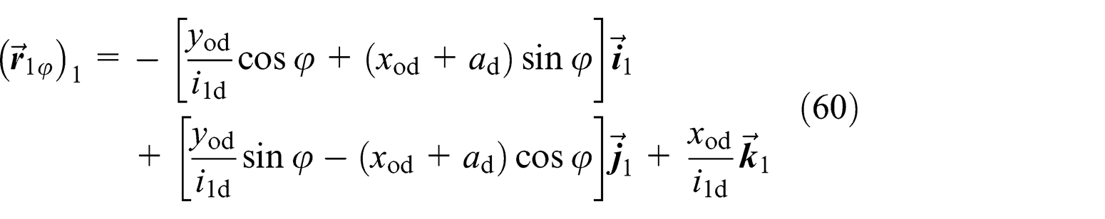
Φ_{φ_{1}} = \frac{\partial Φ}{\partial φ_{1}} = \frac{1}{i_{12} D} [A \cos (φ_{1} - φ) - B \sin (φ_{1} - φ)]

(72)

According to equation (23), the normal vector of the instantaneous contact line of the modified Hindley worm pair can be expressed in $σ_{P}$ as

{(\vec{N})}_{o 1} = N_{ξ} {({\vec{α}}_{ξ})}_{o 1} + N_{η} {({\vec{α}}_{η})}_{o 1}

(73)

where

N_{ξ} = τ_{ξ}^{(1)} {({\vec{V}}_{12})}_{o 1} • {({\vec{α}}_{η})}_{o 1} + {({\vec{ω}}_{12})}_{o 1} • {({\vec{α}}_{η})}_{o 1}

N_{η} = τ_{ξ}^{(1)} {({\vec{V}}_{12})}_{o 1} • {(\vec{α_{ξ}})}_{o 1} + 2 H^{(1)} {({\vec{V}}_{12})}_{o 1} • {(\vec{α_{η}})}_{o 1} - {(\vec{ω_{12}})}_{o 1} • {(\vec{α_{ξ}})}_{o 1}

On the strength of equations (66)–(69), the dot products in the expressions of $N_{ξ}$ and $N_{η}$ in equation (73) can be worked out one by one as follows

\begin{array}{l} {({\vec{V}}_{12})}_{o 1} • {(\vec{α_{ξ}})}_{o 1} = \frac{x_{o 1} - a}{i_{12}} \sin φ_{d} - \frac{\cos φ_{d}}{i_{12}} \\ [i_{12} x_{o 1} \sin (φ_{1} - φ) + (y_{od} - i_{12} y_{o 1}) \cos (φ_{1} - φ)] \end{array}

\begin{array}{l} {({\vec{V}}_{12})}_{o 1} • {(\vec{α_{η}})}_{o 1} = α_{ox} (\frac{y_{od}}{i_{12}} - y_{o 1}) \\ + α_{oy} x_{o 1} - α_{η z} \frac{x_{o 1} - a}{i_{12}} \end{array}

\begin{array}{l} {(\vec{ω_{12}})}_{o 1} • {(\vec{α_{ξ}})}_{o 1} = - \sin φ_{d} - \frac{\sin (φ_{1} - φ)}{i_{12}} \cos φ_{d}, \\ {(\vec{ω_{12}})}_{o 1} • {(\vec{α_{η}})}_{o 1} = \frac{α_{oy}}{i_{12}} + α_{η z} \end{array}

According to equation (12), the curvature interference limit function of the modified Hindley worm gearing can be acquired as

Ψ = N_{ξ} {({\vec{V}}_{12})}_{o 1} • {({\vec{α}}_{ξ})}_{o 1} + N_{η} {({\vec{V}}_{12})}_{o 1} • {({\vec{α}}_{η})}_{o 1} + Φ_{φ_{1}}

(74)

Induced curvature parameters

After ascertaining $\vec{N}$ in $σ_{P}$ in equation (73), the induced geodesic torsion along an arbitrary direction can be obtained from equation (44) or (48). According to the theory expounded in section “Induced principal directions and induced principal curvatures,” the two induced principal directions of the modified Hindley worm drive are the tangential direction of the instantaneous contact line and its normal direction. According to the theory and method advanced in section “Induced principal directions and induced principal curvatures,” the induced principal curvature can be reaped from equation (54) since the normal vector of the instantaneous contact line, $\vec{N}$ , in equation (73) is expressed in $σ_{P}$ .

Numerical outcome and discussion

Parameters of modified Hindley worm drive

The main design parameters of the Hindley worm drive under consideration are $a = 400 mm$ , $i_{12} = 20$ , and $Z_{1} = 2$ . Here, $Z_{1}$ is the number of worm thread.

The modification parameters are $Δ a = - 0.1 mm$ and $Δ i = 0$ . In other words, the involved worm pair pertains to the so-called type I drive.^39–41

Outcome and discussion

As for a type I drive, the meshing limit line is of existence on the worm helical surface $Σ_{1}$ and can be figured down by letting $Φ_{φ_{1}} = 0$ , which is depicted as the line $EF$ in Figure 6. On the helicoidal surface of the modified worm, the position of the meshing limit line approximately ascertains the working length of the worm thread.

Figure 6.

Conjugate zone and contact lines of modified Hindley worm drive: (a) projection drawing of conjugate zone and contact lines on worm helicoids and (b) conjugate zone and contact lines on worm gear tooth surface.

As Figure 6(b) shows, the whole tooth surface of the worm gear is divided into two parts. One part is the conjugate zone $A' B' BA$ and the other part, locating on the both sides of the conjugate zone $A' B' BA$ , may be called the front transition surface, which is formed by the scraping action of the first cutting blade at the inlet portion of the toroidal hob. Of course, such a toroidal hob is completely identical to the corresponding modified Hindley worm.

On the worm gear tooth flank, the lines $AB$ and $A' B'$ stand for the inlet end of the worm and the line $EF$ is the conjugate line of the meshing limit line, which splits up the whole conjugate zone $A' B' BA$ into two sub-conjugated zones. One is the zone $EFBA$ (denoted by a notation $Σ_{2 A}$ ) and the other is $A' B' FE$ (denoted by a notation $Σ_{2 B}$ ).

After the value of the angle $φ_{d}$ is preset, two instantaneous contact lines can be determined in the sub-conjugated zones $Σ_{2 A}$ and $Σ_{2 B}$ , respectively. After changing the value of $φ_{d}$ , two families of the instantaneous contact line can be attained separately in $Σ_{2 A}$ and $Σ_{2 B}$ . The contact lines in $Σ_{2 A}$ are numbered from 1 to 4 while those in $Σ_{2 B}$ are numbered from 1′ to 4′.

Along every contact line, from the top to the root of the worm gear tooth, three meshing points are selected in turn, which are designated by the letters a, b, and c. At every meshing point, after the value of the angle $φ_{d}$ is given in accordance with the contact line, the parameter $φ_{1}$ can be expressed as a function with respect to $u$ by employing the meshing equation $Φ = 0$ . A nonlinear equation with respect to $u$ can then be obtained in the light of the position of the instantaneous meshing point in question. The value of $u$ can be acquired by solving such a nonlinear equation iteratively as well as the value of $φ_{1}$ can be worked out. As a consequence, one meshing point can be determined and the other meshing points can also be determined in line with the same procedure and approach. All the acquired results are supplied in Table 1.

Table 1.

Computing results of $u$ (mm), $φ_{d}$ (°), $φ_{1}$ (°), and $k_{N}^{(12)}$ (1/mm).

		1′	2′	3′	4′	4	3	2	1
	$φ_{d}$	$7 \circ$	$11 \circ$	$15 \circ$	$19 \circ$	$19 \circ$	$15 \circ$	$11 \circ$	$7 \circ$
a	$u$	323.4782	325.7881	324.9678	324.7637	324.7559	324.7560	324.7570	324.7586
	$φ_{1}$	1.8779	3.3318	4.8869	6.5180	0.3181	−1.0562	−2.4492	−3.8443
	$k_{N}^{(12)}$	0.0058	0.0045	0.0020	2.2448e−04	4.2501e−04	0.0428	0.2311	0.9284
b	$u$	310.5053	309.6158	309.2360	309.1300	309.1250	309.1251	309.1263	309.1280
	$φ_{1}$	2.0495	3.5207	5.0109	6.5470	0.3170	−1.0583	−2.4509	−3.8456
	$k_{N}^{(12)}$	0.0038	0.0026	0.0013	1.6145e−04	2.6263e−04	0.0195	0.0918	0.3019
c	$u$	297.6397	297.6379	297.6366	297.6358	297.6358	297.6366	297.6379	297.6397
	$φ_{1}$	2.1576	3.6033	5.0659	6.5672	0.3130	−1.0600	−2.4522	−3.8467
	$k_{N}^{(12)}$	0.0028	0.0020	0.0011	8.0880e−05	8.5796e−05	0.0116	0.0511	0.1547

After determining the values of $u$ , $φ_{d}$ , and $φ_{1}$ , the values of $k_{N}^{(12)}$ at the selected instantaneous meshing points can be ciphered out conveniently from the formulae developed in sections “Induced geodesic torsion and induced principal directions” and “Induced curvature parameter computation for modified Hindley worm drive” and the obtained results are also listed in Table 1.

In the light of the data provided in Table 1, it is easy to verify $n_{1 z} > 0$ from equation (62). In view of this, ${\vec{n}}_{1}$ points from the space to the entity of the worm. In such a case, no curvature interference happens for the numerical example due to $k_{N}^{(12)} > 0$ in the whole conjugate zone as shown by the data in Table 1.

The data in Table 1 also indicate that the values of $k_{N}^{(12)}$ in $Σ_{2 B}$ generally are smaller than those in $Σ_{2 A}$ . This implies that the contact stress level in $Σ_{2 B}$ is lower in line with the principle set forth in section “Induced principal directions and induced principal curvatures.” On the other hand, in both $Σ_{2 A}$ and $Σ_{2 B}$ , the smaller $k_{N}^{(12)}$ becomes visible near the line $EF$ . The smallest $k_{N}^{(12)}$ appears near the point $F$ while the biggest $k_{N}^{(12)}$ appears near the point $A$ in $Σ_{2 A}$ , where the contact stress level consistently is the highest on the tooth surface of the worm gear.

Conclusion

The full work of this study discloses the core role and the fundamental position of the normal vector of the instantaneous contact line in the meshing theory for the line-conjugate tooth surfaces. The normal vector of the instantaneous contact line is connected with not only the curvature interference limit function but also the induced normal curvature, the induced geodesic torsion, the induced principal direction, the induced principal curvature, and so on.

Given this, the computing methodology for the normal vector of the instantaneous contact line is worthy of being investigated deeply. Therewithal, the computing formulae in different form are suggested for the normal vector of the instantaneous contact line in order for convenient use.

Based on this, the formulae for the induced curvature parameters are accordingly given out. In contrast with the previous work, the deducing process is more rigorous and more succinct as well as the obtained results are more practical. Concurrently, different deducing techniques are provided and this is beneficial for the development of the meshing theory for gear drives.

As an application of the theory and methodology put forward, the computation of the induced curvature parameters for the modified Hindley worm drive is taken into account. Some basic and important equations, including the normal vector of the instantaneous contact line, the meshing function, the meshing limit functions, and the induced principal curvature, are achieved for the worm drive.

The numerical example is a type I drive, whose whole conjugate zone on the worm gear tooth flank can be divided into two parts by the conjugate line of the meshing limit line. In one sub-conjugate zone, the value of the induced principal curvature is much smaller than that in the other one. The biggest induced principal curvature comes into view about at the inlet portion of the worm, and certainly the highest contact stress between the teeth also happens roughly at that position.

Footnotes

Appendix 1

Handling Editor: Yangmin Li

Declaration of conflicting interests

The author(s) declared no potential conflicts of interest with respect to the research, authorship, and/or publication of this article.

Funding

The author(s) disclosed receipt of the following financial support for the research, authorship, and/or publication of this article: The research work in this paper was fully supported by National Natural Science Foundation of China under Grant No. 51475083, New Century Excellent Talents Project by Education Ministry of China under Grant No. NCET-13-0116, the Fundamental Research Funds for the Central Universities under Grant No. N160304012, and National Key Basic Research Development Plan of China (the 973 Program) under Grant No. 2014CB046303.

References

Zeng

. Design and processing of spiral bevel gear. Harbin, China: Harbin Institute of Technology Press, 1989 (in Chinese).

Dong

. Design and manufacture of epicycloidal bevel and hypoid gears. Beijing, China: China Machine Press, 2003 (in Chinese).

Johnson

. Contact mechanics. Cambridge: Cambridge University Press, 1985.

Zhu

Zhongkai

Cai

et al . Analysis of load capacity for gears. Beijing, China: Higher Education Press, 1992 (in Chinese).

Wen

Yang

. Elasto-hydrodynamic lubrication. Beijing, China: Tsinghua University Press, 1992 (in Chinese).

Wildhaber

. Meshing theory of spiral bevel and hypoid gear drives (trans. Z

Zhang

). Beijing, China: China Machine Press, 1958 (in Chinese).

Baxter

. Chapter 1: basic theory of gear-tooth action and generation. In: Dudley

(ed.) Gear handbook: the design, manufacture and application of gears. New York: McGraw-Hill Education, 1962, pp.1-1–1-21.

Dyson

. A general theory of the kinematics and geometry of gears in three dimensions. Oxford: Clarendon Press, 1969.

Chen

. Principle of conjugate surfaces, vols 1 and 2. Beijing, China: Science Press, 1974; 1977 (in Chinese).

10.

Sakai

. Takao Sakai anthology (trans. Y

). Shenyang, China: Shenyang Municipal Association for Science and Technology, 1984 (in Chinese).

11.

Litvin

. Meshing principle for gear drives (trans. Lu

Gao

Wang

, 1984). 2nd ed. Shanghai, China: Shanghai Science and Technology Press, 1968 (in Chinese).

12.

Litvin

Fuentes

. Gear geometry and applied theory. 2nd ed. Cambridge: Cambridge University Press, 2004.

13.

Luo

. Meshing theory for gear drives. Beijing, China: Science Press, 1985 (in Chinese).

14.

. Spatial meshing theory and its application, vols. 1 and 2. Beijing, China: Coal Industry Press, 1987 (in Chinese).

15.

Chen

Tang

. Differential geometry and its application in mechanical engineering. Harbin, China: Harbin Institute of Technology Press, 1998 (in Chinese).

16.

. Differential geometry and meshing principle for gear drives. Dongying, China: University of Petroleum Press, 1999 (in Chinese).

17.

Wang

. A simple course on meshing theory for gear drives. Tianjin, China: Tianjin University Press, 2005 (in Chinese).

18.

. Spatial geometry modeling and its application in engineering. Beijing, China: Higher Education Press, 2007 (in Chinese).

19.

. Meshing principle of gear drives. 1st and 2nd ed. Xi’an, China: Xi’an Jiaotong University Press, 1982; 2009 (in Chinese).

20.

Chen

. Meshing theory for gear drives. Beijing, China: Coal Industry Press, 1986 (in Chinese).

21.

Dong

. Foundation of meshing theory for gear drives. Beijing, China: China Machine Press, 1989 (in Chinese).

22.

Dooner

Seireg

. The kinematic geometry of gearing. Hoboken, NJ: John Wiley & Sons, 1995.

23.

Chen

. Curvatures and sliding ratios of conjugate surfaces. ASME J Mech Des 1998; 120: 126–132.

24.

Dong

Ting

et al . Differential contact path and conjugate properties of planar gearing transmission. ASME J Mech Des 2012; 134: 061010.

25.

Radzevich

. Theory of gearing: kinematics, geometry and synthesis. Boca Raton, FL: CRC Press, 2012.

26.

Buckingham

. Analytical mechanics of gears. 3rd ed. New York: Dover Publications Inc., 1988.

27.

Crosher

. Design and application of the worm gear. New York: ASME Press, 2002.

28.

Litvin

. Development of gear technology and theory of gearing. Cleveland, OH: NASA Reference Publication, 1997.

29.

Dudas

. The theory and practice of worm gear drives. London: Penton Press, 2000.

30.

Zhao

Zhang

. Advances in the research of hourglass worm drives. In: Proceedings of international symposium theory and practice of gearing, Izhevsk, Russia, 21–23 January 2014, Kalashnikov Izhevsk State Technical University, IFToMM.

31.

Editorial Committee for Gear Handbook. Gear handbook, vols 1 and 2. 2nd ed. Beijing, China: China Machine Press, 2004 (in Chinese).

32.

Dong

. Design of worm drives, vol. 2. Beijing, China: China Machine Press, 1987 (in Chinese).

33.

Zhao

Yang

et al . Novel types of worm drive. Xi’an, China: Shaanxi Science and Technology Press, 1990 (in Chinese).

34.

Zhou

. Modification principle and manufacturing technology of hourglass worm drives. Changsha, China: National University of Defense Technology Press, 2005 (in Chinese).

35.

Dong

. Design and modification of hourglass worm drives. Beijing, China: China Machine Press, 2004 (in Chinese).

36.

. Lecture notes on differential geometry. 4th ed. Beijing, China: The People’s Education Press, 1982 (in Chinese).

37.

Zhao

Zhang

. Determination of the most dangerous meshing point for modified hourglass worm drives. ASME J Mech Des 2013; 135: 034503.

38.

Zhao

Zhang

. Novel methods for curvature analysis and their application to TA worm. Mech Mach Theory 2016; 97: 155–170.

39.

Zhao

Kong

et al . Tooth flank modification theory of dual-torus double-enveloping hourglass worm drives. Comput Aided Design 2011; 43: 1535–1544.

40.

Zhao

. A general modification theory for double-enveloping hourglass worm drives. Key Eng Mater 2011; 486: 279–282.

41.

Zhao

Zhang

. Computer aided analysis on the meshing behavior of a height-modified dual-torus double-enveloping toroidal worm drive. Comput Aided Design 2010; 43: 1232–1240.

Computing method for induced curvature parameters based on normal vector of instantaneous contact line and its application to Hindley worm pair

Abstract

Keywords

Introduction

Equation of generated tooth surface and partial derivatives of meshing function

Singular point condition of envelope and elicitation of normal vector of instantaneous contact line

Singular point condition of envelope

Elicitation of normal vector of instantaneous contact line

Diverse expressions for normal vector of instantaneous contact line

In principal coordinate frame

In arbitrary unit orthogonal frame

In velocity coordinate frame

Representation based on derivative of unit normal vector

Induced normal curvature of line-conjugate surface couple

Preparative relation expressions

Deducing process of induced normal curvature formula

Affiliated outcomes

Induced geodesic torsion and induced principal directions

Induced geodesic torsion formula

Induced principal directions and induced principal curvatures

Induced curvature parameter computation for modified Hindley worm drive

Equation of worm helicoid and its unit normal vector

Curvature parameters of worm helicoid and moving frame on it

Relative motion

Meshing function of worm pair and tooth surface equation of worm gear

Meshing parameters

Induced curvature parameters

Numerical outcome and discussion

Parameters of modified Hindley worm drive

Outcome and discussion

Conclusion

Footnotes

Appendix 1

Declaration of conflicting interests

Funding

References