Sage Journals: Discover world-class research

Abstract

Various industries, including automobiles, wind power, railroads, airlines, and defense, have their own individual low-temperature test specifications. Since the performance of a test object has to be evaluated after cooling in a climate-controlled chamber, the process consumes an enormous amount of energy and a long time is needed to cool the object. Reducing energy consumption and increasing the cooling rate would offer a huge environmental and economic benefit. This study analyzed the cooling rate and energy consumption of a cryogenic chamber in terms of the ventilation methods and locations of test objects through computational fluid dynamics analysis. In order to calculate energy consumption, the study fixed the compressor power of the refrigerator and created an energy model in the form of a user-defined function that considered changes in the outlet mass flow and refrigerator coefficient of performance according to changes in outlet temperatures within the chamber; this model is used for numerical analysis. The chamber used for the upper air supply and lower exhaust method (Case A) demonstrated a faster cooling rate by 0%–32% compared to the upper air supply and lower exhaust on the opposite face method (Case B) and the upper air supply and central exhaust on the opposite face method (Case F). Case A generally consumed less energy during cooling, whereas Case F consumed the least amount of energy for 4–6 out of the 12 test object locations. Cases A, B, and F demonstrated the highest cooling rates and the lowest energy consumptions when the test object was located at P5 or P11 opposite of the air supply. The cooling rate of the test object and energy consumption should be considered in the ventilation design of a cryogenic test chamber. In the case of a pre-installed chamber, a proper location should be selected for cooling the test object for fast cooling according to the chamber ventilation method.

Keywords

Computational fluid dynamics analysis cryogenic chamber extreme climate mixing ventilation energy efficiency cooling performance

Introduction

Generally, cryogenic tests are tests that evaluate the reliability of products in cryogenic environmental conditions during storage, transportation, and operation. The international/domestic standards related to cryogenic tests vary according to product type. Independent standards are set for cryogenic testing in the automobile, wind power, railroad, airline, military industries, and so on. The temperature condition required for cryogenic testing differs on the basis of product type but is usually set around 233 K. There are also various types of chambers used in tests according to the standards for specific product types. Various studies have been conducted to test the air and thermal flow in chambers.

Gan performed a numerical study by simulating a situation in where there is one occupant in an office space of 4.9 (L) × 3.7 (W) × 2.75 (H). The interpretation is a three-dimensional (3D) model, and the turbulence model is a k–ε model. Five cases were analyzed for heating and eight cases for cooling with the position of the air supply, size of the air supply opening, and position of the exhaust port as variables.¹ Schalin and Nielsen analyzed the chambers of various other cases with different horizontal, vertical, and height ratios. All analytical cases have the form of the upper air supply—air supply and exhaust of the lower exhaust of the opposite side. k–ε and Reynolds stress models (RSM) were used for turbulence models and for the RSM model, various option values were analyzed as variables. In most chambers, the analytical value of the k–ε turbulence model was more suitable for the flow of the air inside the chamber than the RSM turbulence model.² Horikiri et al.³ conducted analytical and comparative research using various turbulence models, measuring the airflow velocity inside chambers with upper supply and lower exhaust. They performed the research that compares four turbulence models (Standard k–ε, re-normalization group (RNG) k–ε, standard k–ω, and shear stress transport (SST) k–ω) based on the experimental results of Nielsen. Both the temperature and flow velocity distributions of the k–ε model demonstrated trends more similar to the experiment result compared to the k–ω model.⁴

Emmerich and McGrattan⁵ conducted analysis and research on the temperature and airflow inside a chamber using large eddy simulation (LES) for a rectangular space with upper supply and lower exhaust. Kolesnikov⁶ conducted analysis using various turbulence models in chambers with upper supply and lower exhaust and compared the test results. G Cao et al.⁷ organized and compared the results of various researches held in various ventilation conditions applicable in office spaces: typical mixing ventilation, displacement ventilation, and a combination of these two. Blay et al.⁸ measured temperatures and velocity in a chamber at a variety of locations at which the upper supply and lower exhaust ports were on opposite sides and where L (length)/H (height) was 1 and compared the result obtained from numerical analysis with the experimental value for the section in the center of the chamber. There have been many studies like the above that are conducted on the airflow and temperature inside chambers under various ventilation conditions, but there has been little progress toward estimating the energy efficiency according to a ventilation method. No studies have evaluated the energy consumption and cooling rate associated with the location of the ventilation method or the test object in an extreme environmental chamber where the temperature status of the test object is important. Since the performance of the test object will be evaluated after cooling to very low temperatures, long hours and enormous amounts of energy are required to cool the test object. Reducing the energy consumption in an extreme environmental chamber, thereby increasing the cooling rate, offers huge environmental and economic benefits. This study evaluated the cooling rate and energy consumption of a chamber in terms of the location of a test object inside it and the ventilation method through analysis of the computational fluid dynamics (CFD). In the study, we discussed the importance of the object-centered chamber design in cryogenic chambers and suggested a methodology that analyzes energy usage of systems using user-defined function (UDF) in the CFD analysis.

Analysis method

Ventilation conditions of the analysis model

In this study, the cryogenic chamber is required to have a rapidly changing temperature. Therefore, the performance of the chamber was analyzed only under mixing ventilation. Among the mixing ventilation methods, ceiling ventilation is used in clean rooms rather than cryogenic chambers and has the advantage of particle control rather than temperature control. Temperature control was an important variable in the cryogenic chamber used in this study; therefore, we focused on the upper and front supply among the mixing ventilation methods instead. The chambers were used in cryogenic tests to simulate the temperature of test objects in cryogenic environments and find out the objects’ operational reliability. Specifications of the chamber were selected by analyzing various cryogenic test standards, and the size of the chamber used for CFD analysis was 6800 × 4600 × 3125 mm³.

The vent was fixed and the refrigeration performance of each cryogenic chamber was analyzed under six ventilation conditions with the test object contained inside the chamber, as shown in Figure 1. The flow rate was identical under all conditions and 90% of the discharge flow rate was sprayed from Inlet 1 in Figure 1. To eliminate the problem of a dead zone being generated in the corner beside the outlet, 10% of the discharge flow rate was sprayed from Inlet 2. For exhaust, the area and location of Outlet 2 was identical, and the location of Outlet 1 differed in six conditions with identical areas. The initial conditions of air circulation inside the chamber are shown in Table 1.

Figure 1.

Location of vent holes for each case: (a) upper supply, lower exhaust, (b) upper supply, lower exhaust at the opposite side, (c) upper supply, upper exhaust on the opposite side, (d) upper supply, lower exhaust on the side, (e) upper supply, upper exhaust on the side, and (f) upper supply, central exhaust on the opposite side.

Table 1.

Operating and initial conditions.

Operating fluid	Air
Initial temperature of all parts (K)	300
Velocity of inlet 1 (m/s)	1.5	2.0	2.5	3.0
Velocity of inlet 2 (m/s)	0.432	0.576	0.72	0.864
Area of inlet 1	0.5375 m²
Area of inlet 2	0.2075 m²
Area of outlet 1	1.755 m²
Area of outlet 2	1.53 m²
Volume flow rate (m³/h)	3225.2	4300.3	5375.3	6450.4
Initial mass flow rate (kg/h)	4031.5	5375.3	6719.2	8063.0
Initial COP	2.6225 (T_C = 313 K, T_E = 273 K, dT = 5 K)
Compressor power (hp)	6	8	10	12
Initial (T_out−T_in)	10.4	10.4	10.4	10.4

COP: coefficient of performance.

Real-time air supply temperature of the analysis model

If the compressor power of a chamber is constant, the coefficient of performance (COP) of the chamber rapidly decreases as the temperature of the air supply decreases. If the wind power of the chamber is constant, the specific volume of the air supply decreases as the temperature decreases and mass flow increases. Formula (1) shows the change in density and mass flow according to temperature

\dot{m} (t) = \frac{p}{R_{specific} . T_{out}} \dot{V}

(1)

The compressor power was assumed to be fixed in the refrigeration system, and the changing COP was expressed in Formula (2) using the results of a study conducted by Lee et al.⁹

COP = 1.0818 - 0.022 T_{c} + 0.0315 T_{e} - 0.0283 Δ T

(2)

Here, the temperature of the refrigerant in the high-compression condenser of the NH3/CO2 cascade refrigeration system was set to 313 K, and the temperature difference between the high-compression condenser and low-compression evaporator was set to 5 K. The temperature of the low-compression evaporator is expressed by

T_{e} = T_{e, min} + \frac{T_{out} - T_{out, min}}{T_{out, max} - T_{out, min}} (T_{e, max} - T_{e, min})

(3)

set to 273 K (T_e,_max)–213 K (T_e,_min) and changed according to the change in air temperature of the chamber outlet, which varied from 300 K (T_out,_max) to 223 K (T_ou_t,min).

Formula (4) expresses the thermal quantity removed during exhaustion of the air supply (A_w = constant)

\overset{\cdot}{Q} = \overset{\cdot}{m} (t) \cdot C \cdot Δ T = \frac{\overset{\cdot}{m} (t)}{{\overset{\cdot}{m}}_{initial}} A_{w} \cdot COP

(4)

Moreover, the mass flow according to the change in exhaust temperature was applied. Formula (5) expresses the temperature difference of exhaust and air supply

Δ T = \frac{\overset{\cdot}{Q}}{\overset{\cdot}{m} (t) \cdot C} = \frac{A_{w} \cdot COP (t_{e})}{{\overset{\cdot}{m}}_{initial} \cdot C}

(5)

The air supply temperature is determined through a series of processes using the exhaust temperature value obtained

T_{in} = T_{out} - Δ T

(6)

The calculations through CFD analysis and of the air supply temperature from that of the chamber exhaust are shown in Figure 2. An UDF of the Fluent 15.0 was used to apply the air supply temperature according to the exhaust temperature change when conducting CFD analysis. When the exhaust temperature reached 223 K, the refrigerator deactivated and the air supply temperature was assumed equivalent to the exhaust temperature. When the exhaust temperature rose to 228 K, the refrigerator was reactivated and the air supply temperature was calculated through the process shown in Figure 2 and applied to the air supply condition. The operation time of the refrigerator was derived by summing up the time when the value of R (on/off value) is equal to 1. The total energy consumption could be calculated because the compressor power was fixed.

Figure 2.

Inlet and outlet temperatures.

Numerical model

The internal and external temperature difference is large in cryogenic chambers and thus it generates thermal loss while the inner chamber is being refrigerated. To assume this type of thermal loss, the conditions related to the chamber boundaries in Table 2 were applied for conductive analysis.

Table 2.

Boundary conditions.

Gage pressure of outlet 1 and outlet 2 (Pa)	−215.6
Material of outside wall	Polyurethane
Thermal conductivity of polyurethane (W/m K)	0.00198
Thickness of outside wall	200 mm
Convective heat transfer coefficient of outside wall (W/m² K)	15
Free stream temperature of outside wall (K)	300

Components used in tests conducted with cryogenic chambers are usually large in size; therefore, the test object used in the analysis was selected on the basis of sizes and materials resembling the state of components usually used in cryogenic tests. Figure 3 shows the location of the test object in the analysis with test objects. The test object in location (Figure 3(c)) was analyzed under all ventilation conditions, and analysis according to the location of the test object was conducted only under the ventilation conditions with the highest refrigerating performances: A, B, and F. The flow directed inside the chamber was set to an abnormal state and non-compressed flow, and the thermal delivery between the test object and internal flow of the chamber was considered using the fluid–structure interaction method. The material properties of the test objects are summarized in Table 3.

Figure 3.

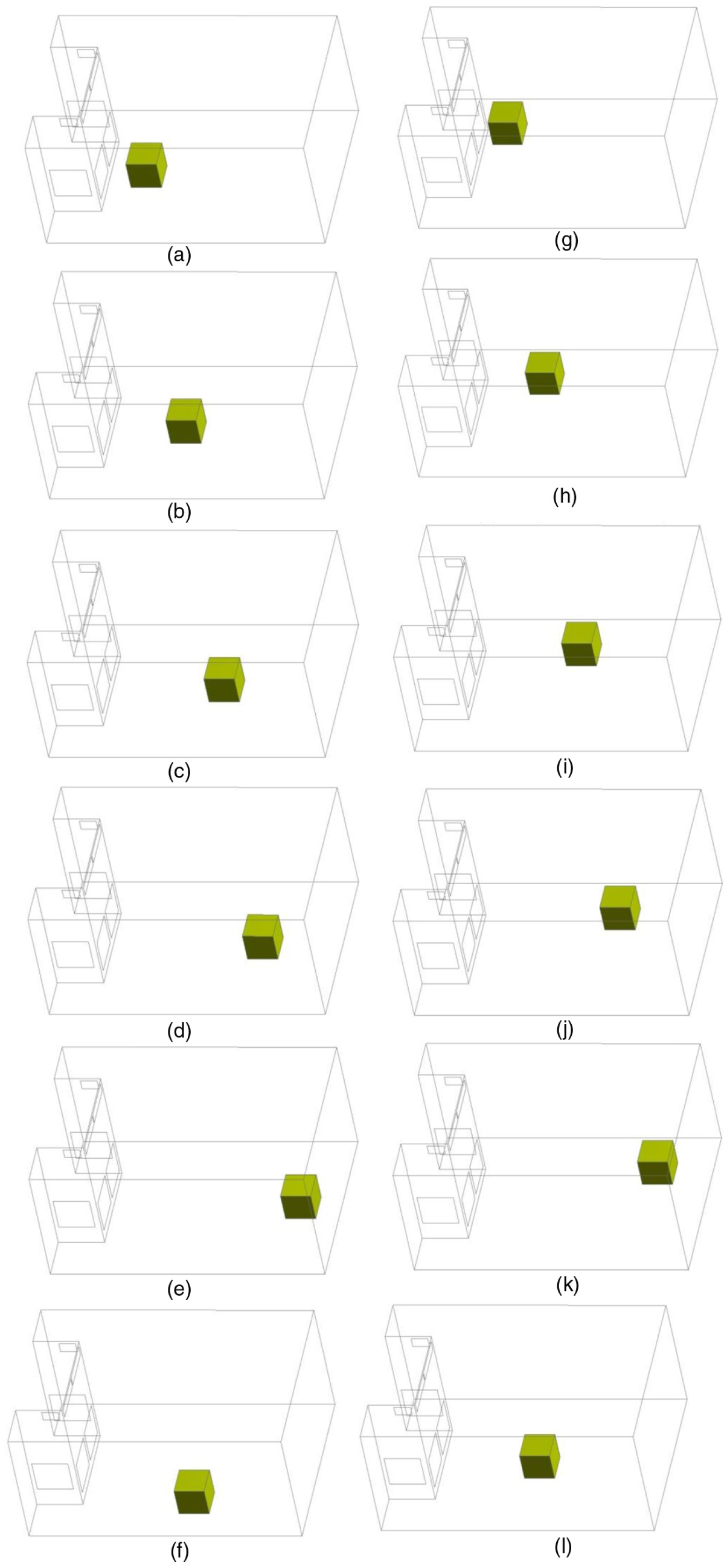
Location of a test object (mm): (a) P1(−1882, 0, 0), (b) P2(−941, 0, 0), (c) P3(0, 0, 0), (d) P4(941, 0, 0), (e) P5(1882, 0, 0), (f) P6(0, −1150, 0), (g) P7(−1882, 0, 1000), (h) P8(−941, 0, 1000), (i) P9(0, 0, 1000), (j) P10(941, 0, 1000), (k) P11(1882, 0, 1000), and (l) P12(0, −1150, 1000).

Table 3.

Material properties of test objects.

Material	Steel
Volume (m³)	0.421875
Density (kg/m³)	8030
Weight (tons)	33.87656
Specific heat (J/kg k)	502.48
Thermal conductivity (W/m k)	16.27

Grid test and turbulence model

Nielsen¹⁰ experimentally studied mixing ventilation conditions (upper supply, lower exhaust at the opposite side); Susin et al. conducted CFD analysis on the experimental models of Nielsen and compared their results. CFD analysis applied standard k–ε, RNG k–ε, and k–ω turbulence models to calculate the airflow distribution in a long room with the following dimensions: height (H) = 3 m, length (L) = 9 m, width (W) = 3 m, inlet height (h) = 0.168 m, outlet height (t) = 0.48 m.¹¹ The inlet boundary conditions were as follows: U = 0.455 m/s, kinematic viscosity (ν) = 15.3 × 10⁻⁶ m²/s, Re_h = hU/ν = 5000.

Susin et al. stated that the standard k–ε model presented the smallest errors for the mean velocity and the fastest computational time. Schalin and Nielsen² carried out a numerical study for a chamber with an L/H of 3 or more and described the k–ε turbulence model as an acceptable model in many situations with room air movement. Blay et al.⁸ experimentally and numerically studied forced convection (upper supply, lower exhaust at the opposite side) conditions and the dimensions of the experiment were as follows: L = 1.04 m, W = 0.3 m, inlet height (h) = 0.018 m, outlet height (t) = 0.024 m. Zuo and Chen¹² conducted fast fluid dynamics (FFD) and CFD analysis on the experimental models of Bay et al. and compared the results. Chen^13,14 used the standard, low Reynolds number, two-layer, two-scale, and RNG k–ε models to conduct CFD analyses on natural convection, forced convection, mixing ventilation, and jet injection and compared the results with the experiment. Chen stated that the results analyzed with the standard and RNG k–ε models under the mixing ventilation condition were reliable.

In this study, ANSYS Fluent V15.0—a commonly used software package—was utilized to conduct CFD analysis on the cryogenic chambers. For the selection of the turbulence model, the model in Figure 4 with experimental results in forced convection (upper supply, lower exhaust at the opposite side) was used. In this simulation, the computed Y⁺ is not allowed to fall below the limit (Y⁺ > 30). The flow velocity measurements in the longitudinal direction of the inlet slot of the chamber are described as within ±5% of the mean value. The experimental values shown in Figure 5 are the flow velocity and temperature measured in the longitudinal direction from the center of the cut surface in the chamber. In this study, the CFD simulations were conducted for a 3D geometry equivalent to Bay et al.’s experiment; thus, the dimensions given in Figure 4 take the following values: L = 1.04 m, W = 0.3 m, inlet height = 0.018 m, outlet height = 0.024 m.

Figure 4.

Dimensions of experiment in a room.

Figure 5.

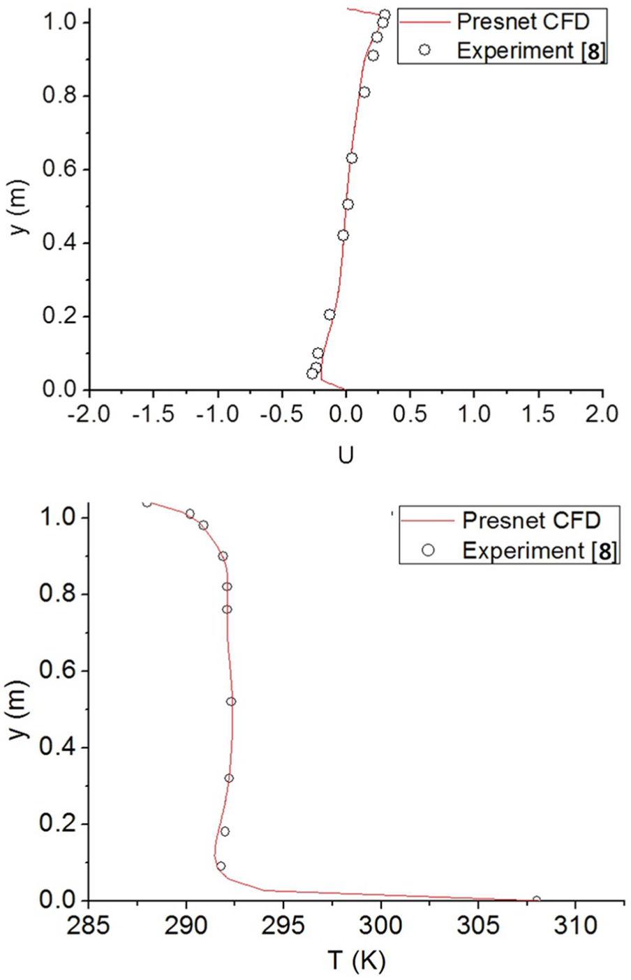
Comparison of air velocity and temperature profiles predicted by CFD with the experimental data: (a) U at x = 0.5 L and (b) T at x = 0.5 L.

The inlet air velocity and temperature were 0.57 m/s and 15°C, respectively. The temperature of the upper, left, and right walls was 15°C, and the temperature of the lower wall was 35.5°C. Figure 5 contains a comparison of experimental values and our computational analysis results regarding the model in Figure 4, and the temperature and velocity profiles were almost identical.

We assumed that the fluid is incompressible and is in the unsteady state. In the numerical analysis, we used the continuity equation, momentum equation, and energy equation as governed equations. These equations are described in equations (7)–(9).

Mass equation

\frac{\partial ρ}{\partial t} + \frac{\partial}{\partial x_{j}} (ρ u_{j}) = 0

(7)

Momentum equation

\frac{\partial}{\partial t} (ρ u_{i}) + \frac{\partial}{\partial x_{j}} (ρ u_{i} u_{j}) = - \frac{\partial p}{\partial x_{i}} + \frac{\partial τ_{ij}}{\partial x_{j}}

(8)

Energy equation

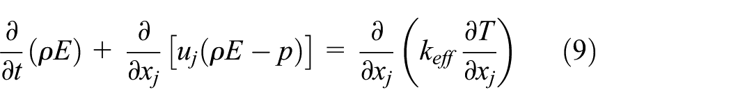
\frac{\partial}{\partial t} (ρ E) + \frac{\partial}{\partial x_{j}} [u_{j} (ρ E - p)] = \frac{\partial}{\partial x_{j}} (k_{eff} \frac{\partial T}{\partial x_{j}})

(9)

where ρ is density, τ is stress tensor, E is total energy, and k_eff is effective thermal conductivity.

The standard k–ε model, with accurate analysis and superior calculation speed, was used as the turbulence model in this study. The standard k–ε model is a two-equation model based on model transport equations for the turbulence kinetic energy (k) and its dissipation rate (ε). The transport equations are as follows

\frac{\partial}{\partial t} (ρ k) + \frac{\partial}{\partial x_{i}} (ρ k u_{i}) = \frac{\partial}{\partial x_{j}} [(μ + \frac{μ_{t}}{σ_{k}}) \frac{\partial k}{\partial x_{j}}] + G_{k} - ρ ε

(10)

\begin{array}{l} \frac{\partial}{\partial t} (ρ ε) + \frac{\partial}{\partial x_{i}} (ρ ε u_{i}) \\ = \frac{\partial}{\partial x_{j}} [(μ + \frac{μ_{t}}{σ_{ε}}) \frac{\partial ε}{\partial x_{j}}] + C_{1 ε} \frac{ε}{k} G_{k} - C_{2 ε} ρ \frac{ε^{2}}{k} \end{array}

(11)

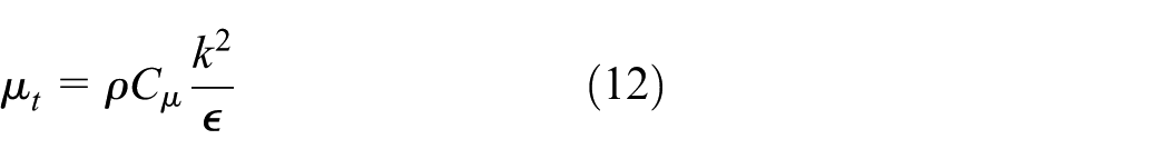
The turbulent viscosity (μ_t) is as follows

μ_{t} = ρ C_{μ} \frac{k^{2}}{ϵ}

(12)

The production of turbulence kinetic energy (G_k) is as follows

G_{k} = - \bar{ρ {u'}_{i} {u'}_{j}} \frac{\partial u_{j}}{\partial x_{i}}

(13)

where, C_1ε = 1.44, C_2ε = 1.92 and C_μ = 0.09 are empirical constants. σ_k = 1.0 and σ_ε = 1.3 are the turbulent Prandtl numbers for k and ε, respectively.¹⁵

The grid test was conducted under the ventilation conditions of Case A. In this study, the simulations have low Reynolds numbers, and therefore, the k–ε turbulence model is used with the standard wall function. The lower bound of Y⁺ limitation for the wall treatment is 30, and when the wall function is used, it is essential to avoid meshes with values lower than 30 as the wall shear stress and the wall heat transfer can and will seriously deteriorate under such conditions.¹⁵

The grid test was conducted within the range of 53,533–275,027 cells, which is in the range with grid densities satisfying the requirement of Y⁺ (Y⁺ > 30). Three points are selected within the chamber for a grid test. The three selected points are where the test objects are generally located inside the chamber. The selected points are placed in an interval of 1 m at the 0.1-m point from the bottom surface of the chamber. Figure 6 illustrates the three points.

Figure 6.

Points for grid test.

Figure 7 illustrates the variation of the velocities of the three points with increase in the number of cells. We can see that there is hardly any change after the number of cells exceeds 120,000. The CFD analysis was implemented for the condition where the cell number was 150,000 or more by reflecting the result of the grid test. Figure 8 is a grid shape created using ANSYS Meshing to analyze a test object at position P3 under the air condition of Case A. The grid shows a quality close to that of a structured grid using the hex-dominant method. The average aspect ratio of the grids is 1.42, and the average skewness is 0.085.

Figure 7.

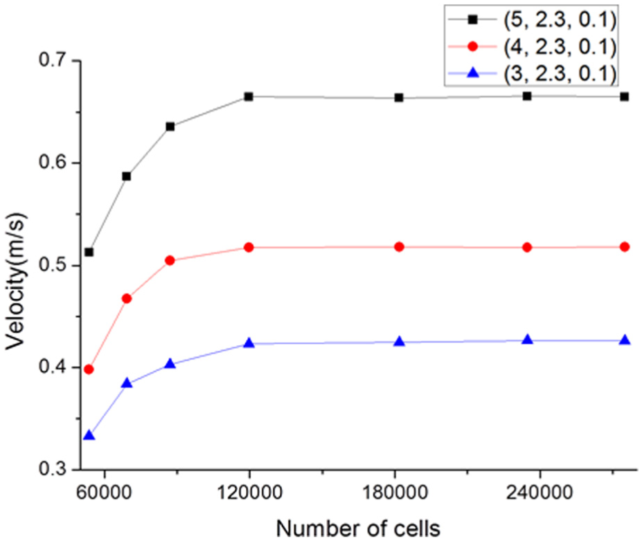
Grid test.

Figure 8.

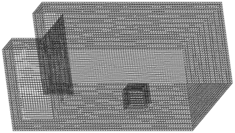
Grid of chamber with test object.

Results

Thermal flow analysis on chambers without test objects

The required compressor power for chambers without test objects was fixed to 6–12 hp for CFD flow analysis. The volume flow rate and velocity are summarized in Table 1. The temperature difference of the inlet and outlet of the evaporator comprises UDF to be determined according to changes in outlet temperatures of the chamber. Therefore, the temperature difference of the inlet and outlet of the evaporator does not change despite increase in volume flow rate.

However, if volume flow rate increases while the temperature difference of the inlet and outlet is maintained, the power required for the compressor will also increase in the same proportion. When the volume flow rate of supply air increases, the cooling rate will be accelerated within the chamber.

Figure 9 show the time spent reaching −40°C according to ventilation method when the compressor power was 6, 8, 10, and 12 hp. Case F had cooling rate values of 18.7%–23.9%, lesser than Case C.

Figure 9.

Time for the internal temperature of the chambers to reach −40°C.

Figure 10 shows the total energy required for the temperature inside the chamber to reach −40°C. Moreover, because the cooling rate increased with the energy consumption of the refrigerator, the time consumed in thermal loss through the chamber boundaries also decreased. The total energy consumption decreased as the refrigerator capacity increased. For the total energy consumption, the difference according to the ventilation method was sustained, regardless of the increasing refrigerator capacity.

Figure 10.

The total energy consumption required for the internal temperature of the chamber to reach −40°C.

The contours of Figure 11 show the velocity (x-direction) in each case. Since the fastest flow within the chamber is around the air supply, the upper airflow has the same direction as the supplied air. However, the bottom part will have a flow in the opposite direction, due to air coming through walls.

Figure 11.

Velocity (x-direction) profiles of the chambers without test object: (a) Case A, (b) Case B, (c) Case C, (d) Case D, (e) Case E, and (f) Case F.

The wide area and low speed with flow opposite from that of the supplied air arises from the fact that there is no aggressive mixing because the air supply remains at the top instead of returning to the bottom. Figure 12 shows temperature distribution in each case. For exhaust air with a low temperature leading to a lower temperature of the supply air, the temperature in the chamber decreases faster. Therefore, Case F has the highest cooling rate because it has the lowest exhaust temperature and a relatively high velocity in the x-direction. Cold air was vigorously mixed in the room, demonstrating significant cooling performance. Conversely, Case C showed the lowest cooling effect because of the high discharge ratio of supply air that could not be mixed in the room. We can see that the cooling effect of the chambers and effective mixing ventilation were significantly correlated.

Figure 12.

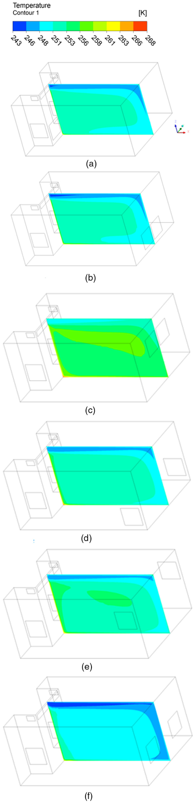
Temperature profiles of the chambers without test object (20 min after operation): (a) Case A, (b) Case B, (c) Case C, (d) Case D, (e) Case E, and (f) Case F.

Analysis of the test object’s refrigeration performance according to its location

For Cases A, B, and F, which had high cooling rates without test objects, CFD flow analysis was conducted in the refrigerator power consumption range of 6–12 hp. Analysis was conducted for ventilation conditions A, B, and F with the test object located at P1–P12.

Figure 13 shows the time required to reach −40°C according to the test object location in Case A. The cooling rate differed by 35.4%–36.5% at maximum according to the test object location when the compressor power was constant. Figure 14 shows the energy required to reach −40°C according to the test object location. The total energy used differed by a maximum of 20.9%–25.5%.

Figure 13.

Time required by test objects to reach −40°C (Case A).

Figure 14.

Total energy consumption required for test objects to reach −40°C (Case A).

Figure 15 shows the time spent to reach −40°C according to the test object location in Case B. The cooling rate differs by 55.6%–58% at maximum according to the test object location when the compressor power is constant. Figure 16 shows the energy consumed to reach −40°C according to the test object location in Case B. The total energy used differs by 28.3%–38.8% at maximum according to the test object location.

Figure 15.

Time required for test object to reach −40°C (Case B).

Figure 16.

Total energy consumption the test objects needs to reach −40°C (Case B).

Figure 17 shows the time required to reach −40°C according to the test object location in Case F. The cooling rate differs by 74.7%–79% at maximum according to the test object location when the compressor power is identical. Figure 18 shows the energy consumed in reaching −40°C according to the test object location in Case F. The total energy used differed by 30.1%–47.7% at maximum. Case A, which had the highest mean velocity (at 12 hp, 0.607 m/s) inside the chamber, had the smallest standard deviation (at 12 hp, 4.97) of the cooling rate according to the test object location. Case F, which had the lowest mean velocity (at 12 hp, 0.519 m/s) inside the chamber, had the largest standard deviation (at 12 hp, 10.30) of the cooling rate.

Figure 17.

Time required by test object to reach −40°C (Case F).

Figure 18.

Total energy consumption required for test object to reach −40°C (Case F).

Figure 19 shows the velocity (z-direction) profile of chambers with the test object 30 min after operation when the test object is located at P11. When the supply airflow affects directly the object, convective heat transfer is increased. For the P11 is located at the position where the supply air directly flows against the object, it shows the highest cooling rate in all three cases.

Figure 19.

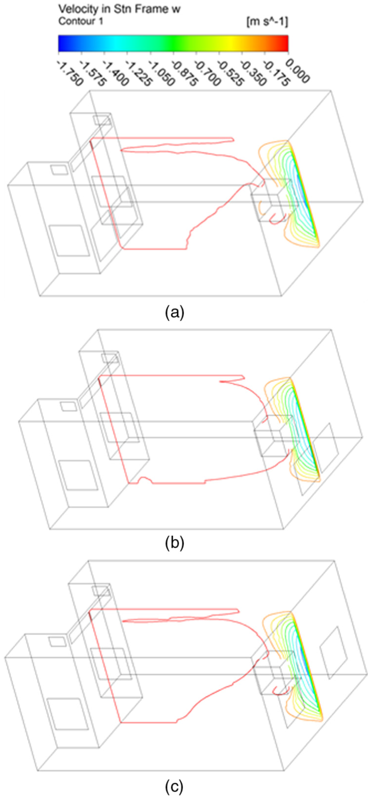
Velocity (z-direction) profiles of the chambers with test object: (a) Case A, (b) Case B, and (c) Case F.

Figures 20 –23 show the time spent reaching −40°C according to test object location when the compressor power was 6, 8, 10, and 12 hp. The inlet flow rate increased by increasing the compressor power, and the deviation value according to test object location decreased as the inlet flow rate increased. When the compressor power was 6, 8, 10, and 12 hp, the cooling rate differed by 0.9%–28.3%, 1.1%–28.4%, 1.25%–28.4%, and 1.3%–32%, respectively, according to the ventilation method. In most locations, the ventilation method in Case A showed a dominant cooling rate, and the tendency was similar even if the flow rate increased. The cooling rate became more efficient when it was closer to the boundary on the other side of the inlet. Moreover, at location P11, Cases A, B, and F had similar cooling rate.

Figure 20.

Time required for test objects to reach −40°C (6 hp).

Figure 21.

Time required for test objects to reach −40°C (8 hp).

Figure 22.

Time required for test objects to reach −40°C (10 hp).

Figure 23.

Time required for test objects to reach −40°C (12 hp).

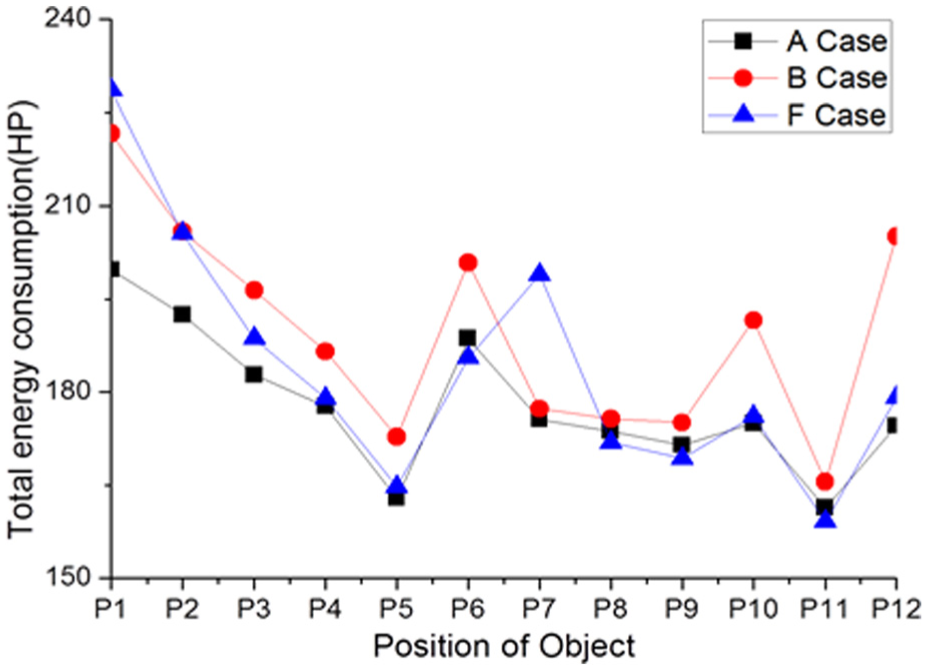
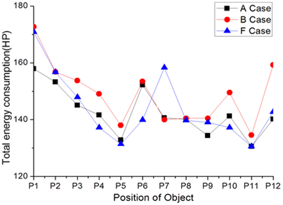
Figures 24 –27 show the energy consumed in reaching −40°C at various test object locations. When the compressor power is 6, 8, 10, and 12 hp, energy consumption differs by 1.9%–17.9%, 2.2%–17.5%, 2.7%–16.8%, and 5.4%–13.6%, respectively, according to the ventilation method. When compared to the results for refrigeration velocity, the deviation value according to ventilation method decreased greatly. In locations P1–P6, the ventilation method of Case A had relatively low energy consumption values. In locations P7–P12, the energy consumption values differed greatly according to compressor power and ventilation method. Similar to the cooling rate, energy consumption became lower as the location neared the boundary on the opposite side of the inlet. The test object located at P11 in Case F had the lowest energy consumption.

Figure 24.

Total energy consumption required by the test objects to reach −40°C (6 hp).

Figure 25.

Total energy consumption required by the test objects to reach −40°C (8 hp).

Figure 26.

Total energy consumption required by the test objects to reach −40°C (10 hp).

Figure 27.

Total energy consumption required by the test objects to reach −40°C (12 hp).

Conclusion

In this study, to evaluate the cooling rate and energy efficiency under different ventilation methods and test object locations, the compressor power of the refrigerator was fixed and a UDF-type energy model was created with consideration of the refrigerator COP and changes in the ventilation mass flow rate according to the outlet temperature change inside the chamber. The model was used for CFD analysis. Because of the fixed inlet area, the compressor capacity of refrigerator was determined according to the inlet velocity in the initial condition. The CFD analysis was conducted with fixed condition of volume flow rate. The temperature difference between air supply and exhaust was calculated by the mass flow rate and COP, which changed according to the outlet temperature. With the compressor power set to 6–12 hp, analysis was conducted on chambers without test objects under ventilation conditions described as Cases A–F and on chambers with test objects at different locations under Cases A, B, and F. The results are listed as follows:

In chambers without test objects, although the temperature reached −40°C, Case F had an energy efficiency of 2.8%–23.9%, higher than the other ventilation conditions.

In ventilation conditions A, B, and F with test objects under identical compressor powers, the cooling rate differed by 35.4%–36.5%, 55.6%–58%, and 74.7%–79%, respectively, according to the test object location.

In ventilation conditions A, B, and F with test objects under identical compressor powers, the total energy consumption differed by 20.9%–25.2%, 28.3%–38.8%, and 30.1%–47.7%, respectively, according to the test object location.

When the compressor power was 6, 8, 10, and 12 hp, the cooling rate differed by 0.9%–28.3%, 1.1%–28.4%, 1.25%–28.4%, and 1.3%–32%, respectively, according to the ventilation method (A, B, and F).

When the compressor power was 6, 8, 10, and 12 hp, the total energy consumption differed by 1.9%–17.9%, 2.2%–17.5%, 2.7%–16.8%, and 5.4%–13.6%, respectively, according to the ventilation method (A, B, and F).

In the analysis conducted according to test object location, the ventilation method with the highest cooling rate and low energy consumption was Case A. Case F showed low cooling rate; however, in a few locations, the energy consumption was very low.

In ventilation conditions A, B, and F, the cooling rate and total energy consumption were the highest in performance when the test object was located at P11. The ventilation method with the highest cooling rate and lowest energy consumption in P11 is Case F.

With the result of the study, we were able to find out the optimal ventilation method in the perspective energy consumption and cooling rate while cooling test objects in the cryogenic chamber (Case A or Case F). In addition, we recognized that a pre-installed chamber also has the optimal location for test objects according to ventilation methods of the chamber when cooling test objects.

Footnotes

Appendix 1

Academic Editor: Luís Godinho

Declaration of conflicting interests

The author(s) declared no potential conflicts of interest with respect to the research, authorship, and/or publication of this article.

Funding

The author(s) disclosed receipt of the following financial support for the research, authorship, and/or publication of this article: This work was supported by the Human Resources Development of Korea Institute of Energy Technology Evaluation and Planning (KETEP) grant funded by the Ministry of Trade, Industry and Energy (No. 20135020910060).

References

Gan

. Evaluation of room air distribution systems using computational fluid dynamics. Energ Buildings 1995; 23: 83–93.

Schalin

Nielsen

. Impact of turbulence anisotropy near walls in room airflow. Indoor Air 2004; 14: 159–168.

Horikiri

Yao

. Numerical simulation of convective airflow in an empty room. Int J Energy Environ 2011; 5: 574–581.

Nielsen

. Specification of a two-dimensional test case. International Energy Agency, energy conservation in buildings and community systems, annex 20: air flow pattern within buildings. Department of Building Technology and Structural Engineering, Aalborg University, 1990, http://vbn.aau.dk/files/197503356/Specification_of_a_TwoDimensional_Test_Case.pdf

Emmerich

McGrattan

. Application of a large eddy simulation model to study room airflow. ASHRAE Trans 1998; 104: 1–9.

Kolesnikov

. Use of computational fluid dynamics to predict airflow and contamination concentration profiles within laboratory floor plan environment. Appl Biosafety 2006; 11: 197–214.

Cao

Awbi

Yao

et al . A review of the performance of different ventilation and airflow distribution systems in buildings. Build Environ 2014; 73: 171–186.

Blay

Mergui

Niculae

. Confined turbulent mixed convection in the presence of horizontal buoyant wall jet. Fundamental Mixed Convect 1992; 213: 65–72.

Lee

T-S

Liu

C-H

Chen

T-W

. Thermodynamic analysis of optimal condensing temperature of cascade-condenser in CO₂/NH₃ cascade refrigeration systems. Int J Refrig 2006; 29: 1100–1108.

10.

Nielsen

. Flow in air conditioned rooms. PhD Thesis, Technical University of Denmark, 1976, http://vbn.aau.dk/files/208635183/FLOW_IN_AIR_CONDITIONED_ROOMS.pdf

11.

Susin

Lindner

Mariani

. Evaluating the influence of the width of inlet slot on the prediction of indoor airflow: comparison with experimental data. Build Environ 2009; 44: 971–986.

12.

Zuo

Chen

. Real-time or faster-than-real-time simulation of airflow in buildings. Indoor Air 2009; 19: 33–44.

13.

Chen

. Comparison of different k–ε models for indoor air-flow computations. Numerical Heat Tr B: Fund 1995; 28: 353–369.

14.

Chen

. Prediction of room air motion by Reynolds-stress models. Build Environ 1996; 31: 233–244.

15.

ANSYS. ANSYS fluent theory guide (Release 15.0). Canonsburg, PA: ANSYS, 2013.

Numerical estimation of energy efficiency in cryogenic chamber with various methods of ventilation and location of test object

Abstract

Keywords

Introduction

Analysis method

Ventilation conditions of the analysis model

Real-time air supply temperature of the analysis model

Numerical model

Grid test and turbulence model

Results

Thermal flow analysis on chambers without test objects

Analysis of the test object’s refrigeration performance according to its location

Conclusion

Footnotes

Appendix 1

Declaration of conflicting interests

Funding

References