Numerical simulation of fuzzy differential equations using general linear method and B-series

Abstract

In this article, numerical simulation of fuzzy differential equations using general linear method is proposed. The significance of general linear method is derivation of algebraic order conditions of method using technique of rooted trees and B-series. Fuzzy general linear method of order 3 based on the concept of generalized Hukuhara differentiability for solving fuzzy differential equations is developed. Convergence of third-order fuzzy general linear method is proven. The proposed method is tested on fuzzy initial value problems, and the numerical results showed that fuzzy general linear method produced more accurate approximation of fuzzy solution for tested problems compared with the existing fuzzy numerical methods.

Introduction

The study of fuzzy differential equations (FDEs) has been interested by many researchers in recent years. FDEs are known as an ideal mathematical modeling of real-world problems whereby uncertainties and randomness exist. Early approaches in FDEs modeling were Hukuhara derivative and differential inclusions. However, they displayed the disadvantage of having fuzzier solutions using those type of differentiability. ¹ Then, generalized Hukuhara differentiability was defined by Bede et al.^1–3 who use the extension of Hukuhara differentiability. The advantage of the generalized Hukuhara differentiability is having solutions of FDEs with decreasing uncertainty. In this work, we use the generalized Hukuhara differentiability given by Bede and Gal. ² A more comprehensive understanding of fuzzy theory and fuzzy logic can be found from Bede. ¹

The analytical solutions of FDEs are difficult to solve; hence, approximating the solutions of first-order linear FDEs using numerical methods has been investigated by many researches. For instance, Ma et al. ⁴ and Abbasbandy and Viranloo ⁵ provided the solutions of FDEs using standard Euler method and Taylor method, respectively. Ghanaie and Moghadam ⁶ and Abbasbandy and Viranloo ⁷ suggested the numerical solutions of FDEs using Runge–Kutta method. Later, fuzzy improved Runge–Kutta method for numerical solution of first-order FDEs was introduced by Rabiei and Ismail. ⁸ Rabiei et al. ⁹ constructed the fuzzy improved Runge–Kutta Nyström method for direct solution of second-order FDEs. Ghazanfari and Shakerami ¹⁰ proposed the numerical solution of FDEs using Runge–Kutta-like method. Moreover, artificial neural network (ANN) method by Effati and Pakdaman, ¹¹ trapezoidal and midpoint methods by Ivaz et al., ¹² and reproducing kernel Hilbert space method by Abu Arqub et al. ¹³ were presented for solving FDEs. Fuzzy fractional differential equation (FFDE) was proposed by Salahshour et al.,^14,15 and Ahmadian et al. ¹⁶ derived the Tau method for solving fuzzy fractional kinetic model.

In Bede, ¹⁷ characterization theorem was introduced to obtain the solution of FDEs by converting them into a system of ordinary differential equations (ODEs). The advantage of this technique is that any numerical method is applicable to solve FDEs. Bede’s characterization theorem was then extended into generalized characterization theorem given by Nieto et al. ¹⁸ under generalized differentiability where the FDEs were translated into the two systems of ODEs. It is found that the FDEs appear in many applications. Several examples include modeling of earthquake engineering vibration problems where the parameters of the ground acceleration have a fuzzy credibilistic nature, and as a result, instead of using classical probabilistic methods, the fuzzy approach is considered to develop the seismic response spectrum. ¹⁹ Besides this, the dynamic beam equation of heat-type equation which inherits uncertainty is represented by the FDEs. ²⁰ The HIV infection is also modeled as fuzzy boundary value problems to minimize the viral load and drug costs. ²¹

General linear method (GLM) was constructed by Butcher^22–24 for numerical solution of first-order ODEs. This method is a linear combination of Runge–Kutta method and multistep method. He used the theory of B-series and different order of rooted trees to construct the algebraic order conditions of GLM. In this article, we considered the GLM as a method with enhancements such as high accuracy.

The first aim of this article is to study the derivation of GLM based on the technique of B-series and rooted trees and obtain the related algebraic order conditions of GLM up to order 4. Then, using the obtained order conditions, we will derive a new set of GLM of order 3. Next and main aim of this research is derivation of fuzzy version of proposed third-order GLM based on the concept of generalized Hukuhara differentiability given by Bede and Gal ² for solving FDEs. The convergence of third-order fuzzy GLM will be proved through the two lemmas and a theorem.

In section “Preliminaries,” basic definitions and theorems on fuzzy sets are provided. In section “GLM,” we present the concept and derivation of the GLM. Section “Third-order fuzzy GLM” contains the fuzzification of GLM for numerical solution of FDEs. Numerical results of GLM compared with the existing numerical methods are provided in section “Numerical results,” and discussion is given in section “Comparison and discussion.” Conclusion is discussed in section “Conclusion.”

Preliminaries

In this section, we present some definitions and notation in the fuzzy settings that will be used in this article.

Definition 1

Let $X$ be a nonempty set. A fuzzy set $u$ in $X$ is characterized by its membership function $u:X\to [0,1]$ : ¹

1. $u$ is normal, there exists $x_0\in \mathbb{R}$ such that $u(x_0)=1$ ;

2. $u$ is a convex fuzzy set, for all $s,r\in \mathbb{R}$ and $t\in [0,1]$ , $u(\mathrm{ts}+(1-t)r)\ge \min \{u(s),u(r)\}$ ;

3. $u$ is upper semicontinuous on $\mathbb{R}$ ;

4. $\mathrm{cl}\{x\in \mathbb{R}|u(x)>0\}$ is compact, where $\mathrm{cl}$ denotes the closure of a subset.

Then, ${\mathbb{R}}_F$ is called the space of fuzzy numbers.

Definition 2

The r-level set of a fuzzy number $u\in {\mathbb{R}}_F$ , $0\le r\le 1$ , denoted by $[u{]}^r$ is defined as ¹

$${\left[u\right]}^r\{\begin{array}{c}\{x\in \mathbb{R}|u\left(x\right)\ge r\},\hfill \\ \multicolumn{1}{c}{\mathrm{cl}\{x\in \mathbb{R}|u\left(x\right)>r\},}\end{array}\begin{array}{c}\mathrm{if}0<r\le 1\hfill \\ \multicolumn{1}{c}{\mathrm{if}r=0}\end{array}$$

It is concluded that the r-level set of a fuzzy number is a closed and bounded interval $[u_1^r,u_2^r]$ , where $u_1^r$ is the lower bound of $[u{]}^r$ and $u_2^r$ indicates the upper bound of $[u{]}^r$ .

Definition 3

The distance $D(u,v)$ between two fuzzy intervals is defined as ¹

$$D(u,v)={\sup }_{\mathrm{r}}\max \{|u_1^r-v_1^r|,|u_2^r-v_2^r|\},r\in [0,1]$$

is the Hausdorff distance between $[u{]}^r$ and $[v{]}^r$ .

Then, it is said that $D$ is a metric in ${\mathbb{R}}_F$ , and the following properties hold:

1. $D(u+w,v+w)=D(u,v),u,v\in {\mathbb{R}}_F$ ;

2. $D(k.u,k.v)=\left|k\right|D(u,v),k\in \mathbb{R},u,v\in {\mathbb{R}}_F$ ;

3. $D(u+v,w+e)\le D(u,w)+D(v,e),u,v,w,e\in {\mathbb{R}}_F$ ;

4. $(D,{\mathbb{R}}_F)$ is a complete metric space.

Definition 4

A function $f:\mathbb{R}\to {\mathbb{R}}_F$ is a fuzzy function if for any fixed arbitrary $t_0\in \mathbb{R}$ and $\epsilon >0$ , $\delta >0$ such that $|t-t_0|<\delta \Rightarrow D(f(t),f(t_0))<\epsilon$ exists, then f is a continuous function. ¹

Definition 5

Let $x,y\in {\mathbb{R}}_F$ . ¹ If there exists $z\in {\mathbb{R}}_F$ such that $x=y\oplus z$ , then $z$ is called the Hukuhara difference (H-difference) of $x$ and $y$ , and it is denoted by $x\ominus y$ (note that $x\ominus y\ne x+(-y)$ ).

Definition 6

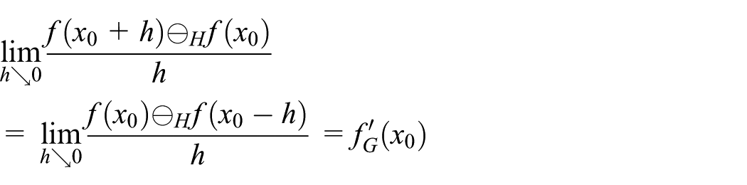
Let $f:[a,b]\to {\mathbb{R}}_F$ and $x_0\in [a,b]$ . ² $f$ is said to be strongly generalized Hukuhara differentiable at $x_0$ if there exists an element $f\prime (x_0)\in {\mathbb{R}}_F$ , such that

• 1. For all $h>0$ sufficiently small, $\exists f(x_0+h)\underset{H}{\ominus }f(x_0),f(x_0)\underset{H}{\ominus }f(x_0-h)$ and the limits (in the metric $D$ )

$$\underset{h\searrow 0}{\lim }\frac{f\left(x_0+h\right){\ominus }_{H}f\left(x_0\right)}{h}=\underset{h\searrow 0}{\lim }\frac{f\left(x_0\right){\ominus }_{H}f\left(x_0-h\right)}{h}={f^{\prime }}_G\left(x_0\right)$$

is known as the $(\mathrm{i})$ differentiability on $(a,b)$ ;

• 2. For all $h>0$ sufficiently small, $\exists f(x_0)\underset{H}{\ominus }f(x_0+h),f(x_0-h)\underset{H}{\ominus }f(x_0)$ and the limits

$$\underset{h\searrow 0}{\lim }\frac{f\left(x_0\right){\ominus }_{H}f\left(x_0+h\right)}{-h}=\underset{h\searrow 0}{\lim }\frac{f\left(x_0-h\right){\ominus }_{H}f\left(x_0\right)}{-h}={f^{\prime }}_G\left(x_0\right)$$

is known as the $(\mathrm{ii})$ differentiability on $(a,b)$ ;

• 3. For all $h>0$ sufficiently small, $\exists f(x_0+h)\underset{H}{\ominus }f(x_0),f(x_0-h)\underset{H}{\ominus }f(x_0)$ and the limits

$$\underset{h\searrow 0}{\lim }\frac{f\left(x_0+h\right){\ominus }_{H}f\left(x_0\right)}{h}=\underset{h\searrow 0}{\lim }\frac{f\left(x_0-h\right){\ominus }_{H}f\left(x_0\right)}{-h}={f^{\prime }}_G\left(x_0\right)$$

• 4. For all $h>0$ sufficiently small, $\exists f(x_0)\underset{H}{\ominus }f(x_0+h),f(x_0)\underset{H}{\ominus }f(x_0-h)$ and the limits

$$\underset{h\searrow 0}{\lim }\frac{f\left(x_0\right){\ominus }_{H}f\left(x_0+h\right)}{-h}=\underset{h\searrow 0}{\lim }\frac{f\left(x_0\right){\ominus }_{H}f\left(x_0-h\right)}{h}={f^{\prime }}_G\left(x_0\right)$$

Theorem 1

Let $f:[a,b]\to {\mathbb{R}}_F$ and $x_0\in [a,b]$ with $f_1^r(x)$ and $f_2^r(x)$ both differentiable at $x_0$ .^1,22 Then

1. $f$ is (i) differentiable at $x_0$ if $[f\prime (x_0)]=[(f_1^r)\prime (x),(f_2^r)\prime (x)],\forall r\in [0,1]$ ;

2. $f$ is (ii) differentiable at $x_0$ if $[f\prime (x_0)]=[(f_2^r)\prime (x),(f_1^r)\prime (x)],\forall r\in [0,1]$ .

Definition 7

Consider the fuzzy initial value problem ¹

$$x\prime \left(t\right)=f(t,x\left(t\right)),x\left(t_0\right)=x_0$$

(1)

where $f:[t_0,T]\times {\mathbb{R}}_F\to {\mathbb{R}}_F$ is a continuous fuzzy mapping and $x_0\in {\mathbb{R}}_F$ and $T$ is a positive number or infinity.

Suppose we have $[x(t){]}^r=[x_1^r(t),x_2^r(t)]$ , and $[f(t,x(t)){]}^r=[f_1^r(t,x_1^r(t),x_2^r(t)),f_2^r(t,x_1^r(t),x_2^r(t))]$

From Theorem 1, if $x(t)$ is $(\mathrm{i})$ differentiable, then equation (1) transfers into the following system of ODEs

$$\{\begin{array}{c}\left(x_1^r\right)\prime \left(t\right)=f_1^r(t,x_1^r\left(t\right),x_2^r\left(t\right)),x_1^r\left(t_0\right)={\left(x_0\right)}_1^r\hfill \\ \multicolumn{1}{c}{\left(x_2^r\right)\prime \left(t\right)=f_2^r(t,x_1^r\left(t\right),x_2^r\left(t\right)),x_2^r\left(t_0\right)={\left(x_0\right)}_2^r}\end{array}$$

(2)

If $x(t)$ is $(\mathrm{ii})$ differentiable, then equation (1) transfers into the following system of ODEs

$$\{\begin{array}{c}{\left(x_1^r\right)}^{\prime }\left(t\right)=f_2^r\left(t,x_1^r\left(t\right),x_2^r\left(t\right)\right),x_1^r\left(t_0\right)={\left(x_0\right)}_1^r\\ {\left(x_2^r\right)}^{\prime }\left(t\right)=f_1^r\left(t,x_1^r\left(t\right),x_2^r\left(t\right)\right),x_2^r\left(t_0\right)={\left(x_0\right)}_2^r\end{array}$$

(3)

General linear method

Consider the first-order initial value problem of ODE given by

$$y\prime \left(x\right)=f(x,y\left(x\right)),y\left(x_0\right)=y_0$$

(4)

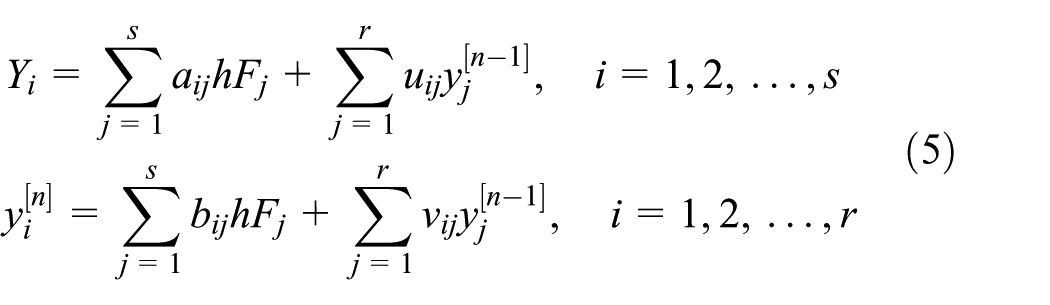
The general formulae for GLM introduced by Butcher^22,23 is given by

$$\begin{array}{c}{Y}_i=\sum _{j=1}^s{a}_{\mathrm{ij}}h{F}_j+\sum _{j=1}^r{u}_{\mathrm{ij}}{y}_j^{[n-1]},i=1,2,\dots ,s\hfill \\ y_i^{\left[n\right]}=\sum _{j=1}^s{b}_{\mathrm{ij}}h{F}_j+\sum _{j=1}^r{v}_{\mathrm{ij}}{y}_j^{[n-1]},i=1,2,\dots ,r\hfill \end{array}$$

(5)

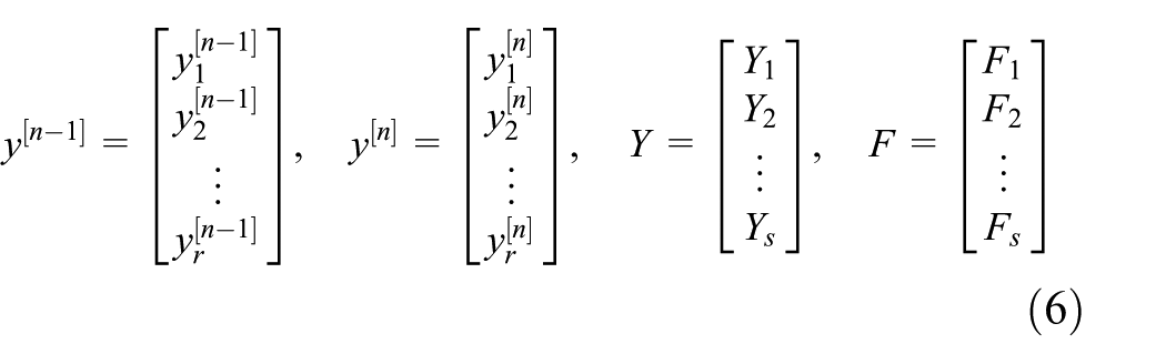
The output approximations from step number $n$ is denoted by $y_i^{[n]}$ , $i=1,2,\dots ,r$ , the stage values by $Y_i=1,2,\dots ,s$ , and the stage derivatives by $F_i=1,2,\dots ,s$ . Simply we could write as below

$$y^{[n-1]}=\left[\begin{array}{c}{y}_1^{[n-1]}\hfill \\ \multicolumn{1}{c}{y_2^{[n-1]}}\\ \multicolumn{1}{c}{⋮}\\ \multicolumn{1}{c}{y_r^{[n-1]}}\end{array}\right],y^{\left[n\right]}=\left[\begin{array}{c}{y}_1^{\left[n\right]}\hfill \\ \multicolumn{1}{c}{y_2^{\left[n\right]}}\\ \multicolumn{1}{c}{⋮}\\ \multicolumn{1}{c}{y_r^{\left[n\right]}}\end{array}\right],Y=\left[\begin{array}{c}{Y}_1\hfill \\ \multicolumn{1}{c}{Y_2}\\ \multicolumn{1}{c}{⋮}\\ \multicolumn{1}{c}{Y_s}\end{array}\right],F=\left[\begin{array}{c}{F}_1\hfill \\ \multicolumn{1}{c}{F_2}\\ \multicolumn{1}{c}{⋮}\\ \multicolumn{1}{c}{F_s}\end{array}\right]$$

(6)

In this section, we derive the new set of coefficients of third-order GLM for numerical solution of first-order ODEs given in equation (4). Then, in the next section, we will develop the fuzzy extension of derived third-order GLM for solving fuzzy initial value problems. Coefficients of GLM using Butcher’s tableau is given in Table 1.

Table 1.

Matrix representation of coefficients of GLM.

$A_{s\times s}$	$U_{s\times r}$
$B_{r\times s}$	$V_{r\times r}$

To further understand the derivation of GLM, a brief introduction on the concept of “rooted trees” is needed. They act as a tool to aid the extraction of order conditions which are required to derive GLM. Rooted trees is defined by Butcher. ²⁴ In this article, we use trees of order 1–4 which are given in Table 2. In addition, we need to mention that the rooted trees are closely associated with the composition law. The composition law plays an important role in construction of various numerical methods such as Runge–Kutta methods, GLM, Rosenbrock methods, multi-derivative methods, and so on. ²⁵ This law permits the derivation of algebraic order conditions in a convenient way avoiding the traditional tedious calculations of Taylor series expansion.

Table 2.

General coefficients of fourth-order GLM.

$0$	$0$	$0$	$u_{11}$	$u_{12}$
$a_{21}$	$0$	$0$	$u_{21}$	$u_{22}$
$a_{31}$	$a_{32}$	$0$	$u_{31}$	$u_{32}$
$b_{11}$	$b_{12}$	$b_{13}$	$1$	$v_{12}$
$b_{21}$	$b_{22}$	$b_{23}$	$v_{21}$	$0$

Definition 8

Let $a:T^{\#}\to \mathbb{R}$ by a mapping, then the form of a formal series given as follows^22,24

$$B(a,y\left(x\right))=a\left(\varnothing \right)y\left(x\right)+\sum _{t\in T}\frac{a\left(t\right)h^{\left|t\right|}}{\sigma \left(t\right)}F\left(t\right)\left(y\left(x\right)\right)$$

(7)

is called the B-series, where $T^{\#}$ denoting the set of rooted trees together with an additional empty tree $\varnothing$ , $a(\varnothing )=1$ and $a(t)=1/\gamma (t)$ ( $\gamma (t)$ is the product over all vertices of the order subtree rooted at that vertex), $\left|t\right|$ is the order of tree, $\sigma (t)$ is the symmetry of tree, $t!$ is the factorial of tree, and $F(t)$ is the elementary differential. To derive the order conditions for GLM, we need to satisfy the theorem below.

Theorem 2

The GLM $(A,U,B,V)$ has order $p$ if there exists $\xi \in X^r$ and $\eta \in X_1^s$ such that for every tree satisfying $r(t)\le p$ ²²

$$\eta \left(t\right)|=A\left(\eta D\right)\left(t\right)+U\xi \left(t\right)$$

(8a)

$$\left(E\xi \right)\left(t\right)|=B\left(\eta D\right)\left(T\right)+V\xi \left(t\right)$$

(8b)

From theorem 2, $\eta$ represents the stages of method, while $E\xi$ is the output approximations computed after a time step. The coefficients of GLM of order 3 with $r=2$ and $s=3$ are given in Table 2.

Here, to derive the order conditions of GLM using equations (8a) and (8b), the values of ${\xi }_t$ and $E{\xi }_t$ for $T^{\#}=\{t_0,t_1,\dots ,t_8\}$ are used as given in Table 3.

Table 3.

Values of ${\xi }_t$ and $E{\xi }_t$ for $t\in T^{\#}$ .

$\mathrm{Tree}$	$t_0=\varnothing$	$t_1=$	$t_2=$	$t_3=$	$t_4=$	$t_5=$	$t_6=$	$t_7=$	$t_8=$
${\xi }_t=\left[\begin{array}{c}{\xi }_1\hfill \\ \multicolumn{1}{c}{{\xi }_2}\end{array}\right]$	$1$	$0$	$0$	$0$	$0$	$0$	$0$	$0$	$0$
	$1$	$-1$	${\xi }_{22}$	${\xi }_{23}$	${\xi }_{24}$	${\xi }_{25}$	${\xi }_{26}$	${\xi }_{27}$	${\xi }_{28}$
$E{\xi }_t=\left[\begin{array}{c}E{\xi }_1\hfill \\ \multicolumn{1}{c}{E{\xi }_2}\end{array}\right]$	$1$	$1$	$\frac{1}{2}$	$\frac{1}{3}$	$\frac{1}{6}$	$\frac{1}{4}$	$\frac{1}{8}$	$\frac{1}{12}$	$\frac{1}{24}$
	$1$	$-1$	$0$	$0$	$0$	$0$	$0$	$0$	$0$

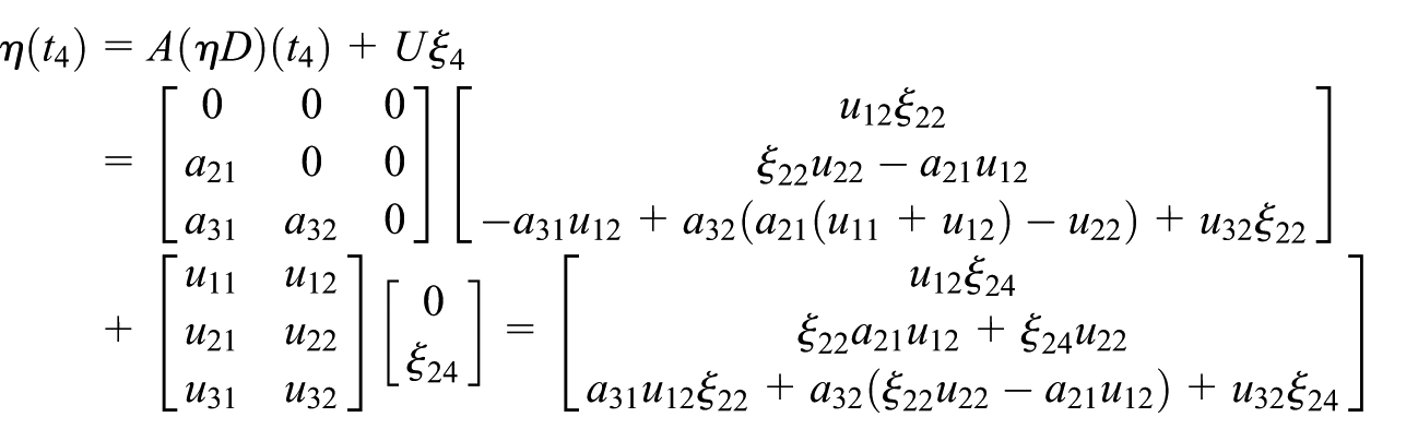
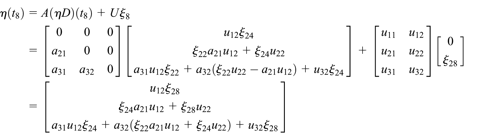
Using formulae of GLM given in equation (8a), the values of $\eta (t)$ for $t\in T^{\#}$ are calculated as follows:

For $t_0=\varnothing$

$$\begin{array}{c}\multicolumn{1}{c}{\eta \left(\varnothing \right)=A\left(\eta D\right)\left(\varnothing \right)+U{\xi }_{\varnothing }}\\ =\left[\begin{array}{ccc}0\hfill & 0\hfill & 0\hfill \\ \multicolumn{1}{c}{a_{21}}& 0\hfill & 0\hfill \\ \multicolumn{1}{c}{a_{31}}& a_{32}\hfill & 0\hfill \end{array}\right]\left[\begin{array}{c}0\hfill \\ \multicolumn{1}{c}{0}\\ \multicolumn{1}{c}{0}\end{array}\right]+\left[\begin{array}{cc}{u}_{11}\hfill & u_{12}\hfill \\ \multicolumn{1}{c}{u_{21}}& u_{22}\hfill \\ \multicolumn{1}{c}{u_{31}}& u_{32}\hfill \end{array}\right]\left[\begin{array}{c}1\hfill \\ \multicolumn{1}{c}{1}\end{array}\right]\hfill \\ =\left[\begin{array}{c}{u}_{11}+u_{12}\hfill \\ \multicolumn{1}{c}{u_{21}+u_{22}}\\ \multicolumn{1}{c}{u_{31}+u_{32}}\end{array}\right]\hfill \end{array}$$

For $t_1=•$

$$\begin{array}{c}\multicolumn{1}{c}{\eta \left(t_1\right)=A\left(\eta D\right)\left(t_1\right)+U{\xi }_1}\\ =\left[\begin{array}{ccc}0\hfill & 0\hfill & 0\hfill \\ \multicolumn{1}{c}{a_{21}}& 0\hfill & 0\hfill \\ \multicolumn{1}{c}{a_{31}}& a_{32}\hfill & 0\hfill \end{array}\right]\left[\begin{array}{c}{u}_{11}+u_{12}\hfill \\ \multicolumn{1}{c}{u_{21}+u_{22}}\\ \multicolumn{1}{c}{u_{31}+u_{32}}\end{array}\right]\hfill \\ +\left[\begin{array}{cc}{u}_{11}\hfill & u_{12}\hfill \\ \multicolumn{1}{c}{u_{21}}& u_{22}\hfill \\ \multicolumn{1}{c}{u_{31}}& u_{32}\hfill \end{array}\right]\left[\begin{array}{c}0\hfill \\ \multicolumn{1}{c}{-1}\end{array}\right]\hfill \\ =\left[\begin{array}{c}-u_{12}\hfill \\ \multicolumn{1}{c}{a_{21}(u_{11}+u_{12})-u_{22}}\\ \multicolumn{1}{c}{a_{31}(u_{11}+u_{12})+a_{32}(u_{21}+u_{22})-u_{32}}\end{array}\right]\hfill \end{array}$$

For $t_2=$

$$\begin{array}{c}\multicolumn{1}{c}{\eta \left(t_2\right)=A\left(\eta D\right)\left(t_2\right)+U{\xi }_2}\\ =\left[\begin{array}{ccc}0\hfill & 0\hfill & 0\hfill \\ \multicolumn{1}{c}{a_{21}}& 0\hfill & 0\hfill \\ \multicolumn{1}{c}{a_{31}}& a_{32}\hfill & 0\hfill \end{array}\right]\hfill \\ \left[\begin{array}{c}-u_{12}\hfill \\ \multicolumn{1}{c}{a_{21}(u_{11}+u_{12})-u_{22}}\\ \multicolumn{1}{c}{a_{31}(u_{11}+u_{12})+a_{32}(u_{21}+u_{22})-u_{32}}\end{array}\right]\hfill \\ +\left[\begin{array}{cc}{u}_{11}\hfill & u_{12}\hfill \\ \multicolumn{1}{c}{u_{21}}& u_{22}\hfill \\ \multicolumn{1}{c}{u_{31}}& u_{32}\hfill \end{array}\right]\left[\begin{array}{c}0\hfill \\ \multicolumn{1}{c}{{\xi }_{22}}\end{array}\right]\hfill \\ =\left[\begin{array}{c}{u}_{12}{\xi }_{22}\hfill \\ \multicolumn{1}{c}{{\xi }_{22}{u}_{22}-a_{21}{u}_{12}}\\ \multicolumn{1}{c}{-a_{31}{u}_{12}+a_{32}(a_{21}(u_{11}+u_{12})-u_{22})+u_{32}{\xi }_{22}}\end{array}\right]\hfill \end{array}$$

For $t_3=$

$$\begin{array}{c}\multicolumn{1}{c}{\eta \left(t_3\right)=A\left(\eta D\right)\left(t_3\right)+U{\xi }_3}\\ =\left[\begin{array}{ccc}0\hfill & 0\hfill & 0\hfill \\ \multicolumn{1}{c}{a_{21}}& 0\hfill & 0\hfill \\ \multicolumn{1}{c}{a_{31}}& a_{32}\hfill & 0\hfill \end{array}\right]\left[\begin{array}{c}{u}_{12}^2\hfill \\ \multicolumn{1}{c}{{(a_{21}(u_{11}+u_{12})-u_{22})}^2}\\ \multicolumn{1}{c}{{(a_{31}(u_{11}+u_{12})+a_{32}(u_{21}+u_{22})-u_{32})}^2}\end{array}\right]\hfill \\ +\left[\begin{array}{cc}{u}_{11}\hfill & u_{12}\hfill \\ \multicolumn{1}{c}{u_{21}}& u_{22}\hfill \\ \multicolumn{1}{c}{u_{31}}& u_{32}\hfill \end{array}\right]\left[\begin{array}{c}0\hfill \\ \multicolumn{1}{c}{{\xi }_{23}}\end{array}\right]=\left[\begin{array}{c}{u}_{12}{\xi }_{23}\hfill \\ \multicolumn{1}{c}{a_{21}{u_{12}}^2+{\xi }_{23}{u}_{22}}\\ \multicolumn{1}{c}{a_{31}{u_{12}}^2+a_{32}{(a_{21}(u_{11}+u_{12})-u_{22})}^2+u_{32}{\xi }_{23}}\end{array}\right]\hfill \end{array}$$

For $t_4=$

$$\begin{array}{c}\multicolumn{1}{c}{\eta \left(t_4\right)=A\left(\eta D\right)\left(t_4\right)+U{\xi }_4}\\ =\left[\begin{array}{ccc}0\hfill & 0\hfill & 0\hfill \\ \multicolumn{1}{c}{a_{21}}& 0\hfill & 0\hfill \\ \multicolumn{1}{c}{a_{31}}& a_{32}\hfill & 0\hfill \end{array}\right]\left[\begin{array}{c}{u}_{12}{\xi }_{22}\hfill \\ \multicolumn{1}{c}{{\xi }_{22}{u}_{22}-a_{21}{u}_{12}}\\ \multicolumn{1}{c}{-a_{31}{u}_{12}+a_{32}(a_{21}(u_{11}+u_{12})-u_{22})+u_{32}{\xi }_{22}}\end{array}\right]\hfill \\ +\left[\begin{array}{cc}{u}_{11}\hfill & u_{12}\hfill \\ \multicolumn{1}{c}{u_{21}}& u_{22}\hfill \\ \multicolumn{1}{c}{u_{31}}& u_{32}\hfill \end{array}\right]\left[\begin{array}{c}0\hfill \\ \multicolumn{1}{c}{{\xi }_{24}}\end{array}\right]=\left[\begin{array}{c}{u}_{12}{\xi }_{24}\hfill \\ \multicolumn{1}{c}{{\xi }_{22}{a}_{21}{u}_{12}+{\xi }_{24}{u}_{22}}\\ \multicolumn{1}{c}{a_{31}{u}_{12}{\xi }_{22}+a_{32}({\xi }_{22}{u}_{22}-a_{21}{u}_{12})+u_{32}{\xi }_{24}}\end{array}\right]\hfill \end{array}$$

For $t_5=$

$$\begin{array}{c}\multicolumn{1}{c}{\eta \left(t_5\right)=A\left(\eta D\right)\left(t_5\right)+U{\xi }_5}\\ =\left[\begin{array}{ccc}0\hfill & 0\hfill & 0\hfill \\ \multicolumn{1}{c}{a_{21}}& 0\hfill & 0\hfill \\ \multicolumn{1}{c}{a_{31}}& a_{32}\hfill & 0\hfill \end{array}\right]\left[\begin{array}{c}-u_{12}^3\hfill \\ \multicolumn{1}{c}{{(a_{21}(u_{11}+u_{12})-u_{22})}^3}\\ \multicolumn{1}{c}{{(a_{31}(u_{11}+u_{12})+a_{32}(u_{21}+u_{22})-u_{32})}^3}\end{array}\right]\hfill \\ +\left[\begin{array}{cc}{u}_{11}\hfill & u_{12}\hfill \\ \multicolumn{1}{c}{u_{21}}& u_{22}\hfill \\ \multicolumn{1}{c}{u_{31}}& u_{32}\hfill \end{array}\right]\left[\begin{array}{c}0\hfill \\ \multicolumn{1}{c}{{\xi }_{25}}\end{array}\right]=\left[\begin{array}{c}{u}_{12}{\xi }_{25}\hfill \\ \multicolumn{1}{c}{-a_{21}{u}_{12}^3+{\xi }_{25}{u}_{22}}\\ \multicolumn{1}{c}{-a_{31}{u}_{12}^3+a_{32}{(a_{21}(u_{11}+u_{12})-u_{22})}^3+u_{32}{\xi }_{25}}\end{array}\right]\hfill \end{array}$$

For $t_6=$

$$\begin{array}{c}\multicolumn{1}{c}{\eta \left(t_6\right)=A\left(\eta D\right)\left(t_6\right)+U{\xi }_6}\\ =\left[\begin{array}{ccc}0\hfill & 0\hfill & 0\hfill \\ \multicolumn{1}{c}{a_{21}}& 0\hfill & 0\hfill \\ \multicolumn{1}{c}{a_{31}}& a_{32}\hfill & 0\hfill \end{array}\right]\left[\begin{array}{c}-u_{12}^2{\xi }_{22}\hfill \\ \multicolumn{1}{c}{(a_{21}(u_{11}+u_{12})-u_{22})({\xi }_{22}{u}_{22}-a_{21}{u}_{12})}\\ \multicolumn{1}{c}{(a_{31}(u_{11}+u_{12})+a_{32}(u_{21}+u_{22})-u_{32})(-a_{31}{u}_{12}+a_{32}(a_{21}(u_{11}+u_{12})-u_{22})+u_{32}{\xi }_{22})}\end{array}\right]\hfill \\ +\left[\begin{array}{cc}{u}_{11}\hfill & u_{12}\hfill \\ \multicolumn{1}{c}{u_{21}}& u_{22}\hfill \\ \multicolumn{1}{c}{u_{31}}& u_{32}\hfill \end{array}\right]\left[\begin{array}{c}0\hfill \\ \multicolumn{1}{c}{{\xi }_{26}}\end{array}\right]=\left[\begin{array}{c}{u}_{12}{\xi }_{26}\hfill \\ \multicolumn{1}{c}{-{\xi }_{22}{a}_{21}{u}_{12}^2+{\xi }_{26}{u}_{22}}\\ \multicolumn{1}{c}{-a_{31}{u}_{12}^2{\xi }_{22}+a_{32}(a_{21}(u_{11}+u_{12})-u_{22})({\xi }_{22}{u}_{22}-a_{21}{u}_{12})+u_{32}{\xi }_{26}}\end{array}\right]\hfill \end{array}$$

For $t_7=$

$$\begin{array}{c}\multicolumn{1}{c}{\eta \left(t_7\right)=A\left(\eta D\right)\left(t_7\right)+U{\xi }_7}\\ =\left[\begin{array}{ccc}0\hfill & 0\hfill & 0\hfill \\ \multicolumn{1}{c}{a_{21}}& 0\hfill & 0\hfill \\ \multicolumn{1}{c}{a_{31}}& a_{32}\hfill & 0\hfill \end{array}\right]\left[\begin{array}{c}{u}_{12}{\xi }_{23}\hfill \\ \multicolumn{1}{c}{a_{21}{u_{12}}^2+{\xi }_{23}{u}_{22}}\\ \multicolumn{1}{c}{a_{31}{u_{12}}^2+a_{32}{(a_{21}(u_{11}+u_{12})-u_{22})}^2+u_{32}{\xi }_{23}}\end{array}\right]+\left[\begin{array}{cc}{u}_{11}\hfill & u_{12}\hfill \\ \multicolumn{1}{c}{u_{21}}& u_{22}\hfill \\ \multicolumn{1}{c}{u_{31}}& u_{32}\hfill \end{array}\right]\left[\begin{array}{c}0\hfill \\ \multicolumn{1}{c}{{\xi }_{27}}\end{array}\right]\hfill \\ =\left[\begin{array}{c}{u}_{12}{\xi }_{27}\hfill \\ \multicolumn{1}{c}{{\xi }_{23}{a}_{21}{u}_{12}+{\xi }_{27}{u}_{22}}\\ \multicolumn{1}{c}{a_{31}{u}_{12}{\xi }_{23}+a_{32}(a_{21}{u_{12}}^2+{\xi }_{23}{u}_{22})+u_{32}{\xi }_{27}}\end{array}\right]\hfill \end{array}$$

For $t_8=$

$$\begin{array}{c}\multicolumn{1}{c}{\eta \left(t_8\right)=A\left(\eta D\right)\left(t_8\right)+U{\xi }_8}\\ =\left[\begin{array}{ccc}0\hfill & 0\hfill & 0\hfill \\ \multicolumn{1}{c}{a_{21}}& 0\hfill & 0\hfill \\ \multicolumn{1}{c}{a_{31}}& a_{32}\hfill & 0\hfill \end{array}\right]\left[\begin{array}{c}{u}_{12}{\xi }_{24}\hfill \\ \multicolumn{1}{c}{{\xi }_{22}{a}_{21}{u}_{12}+{\xi }_{24}{u}_{22}}\\ \multicolumn{1}{c}{a_{31}{u}_{12}{\xi }_{22}+a_{32}({\xi }_{22}{u}_{22}-a_{21}{u}_{12})+u_{32}{\xi }_{24}}\end{array}\right]+\left[\begin{array}{cc}{u}_{11}\hfill & u_{12}\hfill \\ \multicolumn{1}{c}{u_{21}}& u_{22}\hfill \\ \multicolumn{1}{c}{u_{31}}& u_{32}\hfill \end{array}\right]\left[\begin{array}{c}0\hfill \\ \multicolumn{1}{c}{{\xi }_{28}}\end{array}\right]\hfill \\ =\left[\begin{array}{c}{u}_{12}{\xi }_{28}\hfill \\ \multicolumn{1}{c}{{\xi }_{24}{a}_{21}{u}_{12}+{\xi }_{28}{u}_{22}}\\ \multicolumn{1}{c}{a_{31}{u}_{12}{\xi }_{24}+a_{32}({\xi }_{22}{a}_{21}{u}_{12}+{\xi }_{24}{u}_{22})+u_{32}{\xi }_{28}}\end{array}\right]\hfill \end{array}$$

Consequently, by substituting the obtained values of $\eta (t)$ into equation (8b), the values of $(E\xi )(t)$ for $T^{\#}=\{t_0,t_1,\dots ,t_8\}$ are given as follows:

For $t_0=\varnothing$

$$\begin{array}{c}\multicolumn{1}{c}{\left(E\xi \right)\left(\varnothing \right)=B\left(\eta D\right)\left(\varnothing \right)+V{\xi }_{\varnothing }}\\ \multicolumn{1}{c}{\left[\begin{array}{c}1\hfill \\ \multicolumn{1}{c}{1}\end{array}\right]=\left[\begin{array}{ccc}{b}_{11}\hfill & b_{12}\hfill & b_{13}\hfill \\ \multicolumn{1}{c}{b_{21}}& b_{22}\hfill & b_{23}\hfill \end{array}\right]\left[\begin{array}{c}0\hfill \\ \multicolumn{1}{c}{0}\\ \multicolumn{1}{c}{0}\end{array}\right]+\left[\begin{array}{cc}1\hfill & v_{12}\hfill \\ \multicolumn{1}{c}{v_{21}}& 0\hfill \end{array}\right]\left[\begin{array}{c}1\hfill \\ \multicolumn{1}{c}{1}\end{array}\right]}\\ =\left[\begin{array}{c}1+v_{12}\hfill \\ \multicolumn{1}{c}{v_{21}}\end{array}\right]\hfill \end{array}$$

For $t_1=$

$$\begin{array}{c}\multicolumn{1}{c}{\left(E\xi \right)\left(t_1\right)=B\left(\eta D\right)\left(t_1\right)+V{\xi }_1}\\ \multicolumn{1}{c}{\left[\begin{array}{c}1\hfill \\ \multicolumn{1}{c}{0}\end{array}\right]=\left[\begin{array}{ccc}{b}_{11}\hfill & b_{12}\hfill & b_{13}\hfill \\ \multicolumn{1}{c}{b_{21}}& b_{22}\hfill & b_{23}\hfill \end{array}\right]\left[\begin{array}{c}{u}_{11}+u_{12}\hfill \\ \multicolumn{1}{c}{u_{21}+u_{22}}\\ \multicolumn{1}{c}{u_{31}+u_{32}}\end{array}\right]+\left[\begin{array}{cc}1\hfill & v_{12}\hfill \\ \multicolumn{1}{c}{v_{21}}& 0\hfill \end{array}\right]\left[\begin{array}{c}0\hfill \\ \multicolumn{1}{c}{-1}\end{array}\right]}\\ =\left[\begin{array}{c}{b}_{11}(u_{11}+u_{12})+b_{12}(u_{21}+u_{22})+b_{13}(u_{31}+u_{32})-v_{12}\hfill \\ \multicolumn{1}{c}{b_{21}(u_{11}+u_{12})+b_{22}(u_{21}+u_{22})+b_{23}(u_{31}+u_{32})}\end{array}\right]\hfill \end{array}$$

For $t_2=$

$$\begin{array}{c}\multicolumn{1}{c}{\left(E\xi \right)\left(t_2\right)=B\left(\eta D\right)\left(t_2\right)+V{\xi }_2}\\ \multicolumn{1}{c}{\left[\begin{array}{c}\frac{1}{2}\hfill \\ \multicolumn{1}{c}{0}\end{array}\right]=\left[\begin{array}{ccc}{b}_{11}\hfill & b_{12}\hfill & b_{13}\hfill \\ \multicolumn{1}{c}{b_{21}}& b_{22}\hfill & b_{23}\hfill \end{array}\right]\left[\begin{array}{c}-u_{12}\hfill \\ \multicolumn{1}{c}{a_{21}(u_{11}+u_{12})-u_{22}}\\ \multicolumn{1}{c}{a_{31}(u_{11}+u_{12})+a_{32}(u_{21}+u_{22})-u_{32}}\end{array}\right]+\left[\begin{array}{cc}1\hfill & v_{12}\hfill \\ \multicolumn{1}{c}{v_{21}}& 0\hfill \end{array}\right]\left[\begin{array}{c}0\hfill \\ \multicolumn{1}{c}{{\xi }_{22}}\end{array}\right]}\\ =\left[\begin{array}{c}-b_{11}{u}_{12}+b_{12}(a_{21}(u_{11}+u_{12})-u_{22})+b_{13}(a_{31}(u_{11}+u_{12})+a_{32}(u_{21}+u_{22})-u_{32})+v_{12}{\xi }_{22}\hfill \\ \multicolumn{1}{c}{-b_{12}{u}_{12}+b_{22}(a_{21}(u_{11}+u_{12})-u_{22})+b_{23}(a_{31}(u_{11}+u_{12})+a_{32}(u_{21}+u_{22})-u_{32})}\end{array}\right]\hfill \end{array}$$

For $t_3=$

$$\begin{array}{c}\multicolumn{1}{c}{\left(E\xi \right)\left(t_3\right)=B\left(\eta D\right)\left(t_3\right)+V{\xi }_3}\\ \multicolumn{1}{c}{\left[\begin{array}{c}\frac{1}{3}\hfill \\ \multicolumn{1}{c}{0}\end{array}\right]=\left[\begin{array}{ccc}{b}_{11}\hfill & b_{12}\hfill & b_{13}\hfill \\ \multicolumn{1}{c}{b_{21}}& b_{22}\hfill & b_{23}\hfill \end{array}\right]\left[\begin{array}{c}{u}_{12}^2\hfill \\ \multicolumn{1}{c}{{(a_{21}(u_{11}+u_{12})-u_{22})}^2}\\ \multicolumn{1}{c}{{(a_{31}(u_{11}+u_{12})+a_{32}(u_{21}+u_{22})-u_{32})}^2}\end{array}\right]+\left[\begin{array}{cc}1\hfill & v_{12}\hfill \\ \multicolumn{1}{c}{v_{21}}& 0\hfill \end{array}\right]\left[\begin{array}{c}0\hfill \\ \multicolumn{1}{c}{{\xi }_{23}}\end{array}\right]}\\ =\left[\begin{array}{c}{b}_{11}{u}_{12}^2+b_{12}{(a_{21}(u_{11}+u_{12})-u_{22})}^2+b_{13}{(a_{31}(u_{11}+u_{12})+a_{32}(u_{21}+u_{22})-u_{32})}^2+v_{12}{\xi }_{23}\hfill \\ \multicolumn{1}{c}{b_{21}{u_{12}}^2+b_{22}{(a_{21}(u_{11}+u_{12})-u_{22})}^2+b_{23}{(a_{31}(u_{11}+u_{12})+a_{32}(u_{21}+u_{22})-u_{32})}^2}\end{array}\right]\hfill \end{array}$$

For $t_4=$

$$\begin{array}{c}\multicolumn{1}{c}{\left(E\xi \right)\left(t_4\right)=B\left(\eta D\right)\left(t_4\right)+V{\xi }_4}\\ \multicolumn{1}{c}{\left[\begin{array}{c}\frac{1}{6}\hfill \\ \multicolumn{1}{c}{0}\end{array}\right]=\left[\begin{array}{ccc}{b}_{11}\hfill & b_{12}\hfill & b_{13}\hfill \\ \multicolumn{1}{c}{b_{21}}& b_{22}\hfill & b_{23}\hfill \end{array}\right]\left[\begin{array}{c}{u}_{12}{\xi }_{22}\hfill \\ \multicolumn{1}{c}{{\xi }_{22}{u}_{22}-a_{21}{u}_{12}}\\ \multicolumn{1}{c}{-a_{31}{u}_{12}+a_{32}(a_{21}(u_{11}+u_{12})-u_{22})+u_{32}{\xi }_{22}}\end{array}\right]+\left[\begin{array}{cc}1\hfill & v_{12}\hfill \\ \multicolumn{1}{c}{v_{21}}& 0\hfill \end{array}\right]\left[\begin{array}{c}0\hfill \\ \multicolumn{1}{c}{{\xi }_{24}}\end{array}\right]}\\ =\left[\begin{array}{c}{b}_{11}{u}_{12}{\xi }_{22}+b_{12}({\xi }_{22}{u}_{22}-a_{21}{u}_{12})+b_{13}(-a_{31}{u}_{12}+a_{32}(a_{21}(u_{11}+u_{12})-u_{22})+u_{32}{\xi }_{22})+v_{12}{\xi }_{24}\hfill \\ \multicolumn{1}{c}{b_{21}{u}_{12}{\xi }_{22}+b_{22}({\xi }_{22}{u}_{22}-a_{21}{u}_{12})+b_{23}(-a_{31}{u}_{12}+a_{32}(a_{21}(u_{11}+u_{12})-u_{22})+u_{32}{\xi }_{22})}\end{array}\right]\hfill \end{array}$$

For $t_5=$

$$\begin{array}{c}\left(E\xi \right)\left(t_5\right)=B\left(\eta D\right)\left(t_5\right)+V{\xi }_5\hfill \\ \left[\begin{array}{c}\frac{1}{4}\hfill \\ \multicolumn{1}{c}{0}\end{array}\right]=\left[\begin{array}{ccc}{b}_{11}\hfill & b_{12}\hfill & b_{13}\hfill \\ \multicolumn{1}{c}{b_{21}}& b_{22}\hfill & b_{23}\hfill \end{array}\right]\left[\begin{array}{c}-u_{12}^3\hfill \\ \multicolumn{1}{c}{{(a_{21}(u_{11}+u_{12})-u_{22})}^3}\\ \multicolumn{1}{c}{{(a_{31}(u_{11}+u_{12})+a_{32}(u_{21}+u_{22})-u_{32})}^3}\end{array}\right]+\left[\begin{array}{cc}1\hfill & v_{12}\hfill \\ \multicolumn{1}{c}{v_{21}}& 0\hfill \end{array}\right]\left[\begin{array}{c}0\hfill \\ \multicolumn{1}{c}{{\xi }_{25}}\end{array}\right]\hfill \\ =\left[\begin{array}{c}-b_{11}{u}_{12}^3+b_{12}{(a_{21}(u_{11}+u_{12})-u_{22})}^3+b_{13}{(a_{31}(u_{11}+u_{12})+a_{32}(u_{21}+u_{22})-u_{32})}^3+v_{12}{\xi }_{25}\hfill \\ \multicolumn{1}{c}{-b_{21}{u}_{12}^3+b_{22}{(a_{21}(u_{11}+u_{12})-u_{22})}^3+b_{23}{(a_{31}(u_{11}+u_{12})+a_{32}(u_{21}+u_{22})-u_{32})}^3}\end{array}\right]\hfill \end{array}$$

For $t_6=$

$$\begin{array}{c}\multicolumn{1}{c}{\left(E\xi \right)\left(t_6\right)=B\left(\eta D\right)\left(t_6\right)+V{\xi }_6}\\ \multicolumn{1}{c}{\left[\begin{array}{c}\frac{1}{8}\hfill \\ \multicolumn{1}{c}{0}\end{array}\right]=\left[\begin{array}{ccc}{b}_{11}\hfill & b_{12}\hfill & b_{13}\hfill \\ \multicolumn{1}{c}{b_{21}}& b_{22}\hfill & b_{23}\hfill \end{array}\right]\left[\begin{array}{c}-u_{12}^2{\xi }_{22}\hfill \\ \multicolumn{1}{c}{(a_{21}(u_{11}+u_{12})-u_{22})({\xi }_{22}{u}_{22}-a_{21}{u}_{12})}\\ \multicolumn{1}{c}{(a_{31}(u_{11}+u_{12})+a_{32}(u_{21}+u_{22})-u_{32})(-a_{31}{u}_{12}+a_{32}(a_{21}(u_{11}+u_{12})-u_{22})+u_{32}{\xi }_{22})}\end{array}\right]}\\ +\left[\begin{array}{cc}1\hfill & v_{12}\hfill \\ \multicolumn{1}{c}{v_{21}}& 0\hfill \end{array}\right]\left[\begin{array}{c}0\hfill \\ \multicolumn{1}{c}{{\xi }_{26}}\end{array}\right]\hfill \\ =\left[\begin{array}{c}-b_{11}{u}_{12}^2{\xi }_{22}+b_{12}(a_{21}(u_{11}+u_{12})-u_{22})({\xi }_{22}{u}_{22}-a_{21}{u}_{12})\hfill \\ \multicolumn{1}{c}{+b_{13}(a_{31}(u_{11}+u_{12})+a_{32}(u_{21}+u_{22})-u_{32})-a_{31}{u}_{12}+a_{32}(a_{21}(u_{11}+u_{12})-u_{22})+v_{12}{\xi }_{26}}\\ \multicolumn{1}{c}{-b_{21}{u}_{12}^2{\xi }_{22}+b_{22}(a_{21}(u_{11}+u_{12})-u_{22})({\xi }_{22}{u}_{22}-a_{21}{u}_{12})}\\ \multicolumn{1}{c}{+b_{23}(a_{31}(u_{11}+u_{12})+a_{32}(u_{21}+u_{22})-u_{32})-a_{31}{u}_{12}+a_{32}(a_{21}(u_{11}+u_{12})-u_{22})}\end{array}\right]\hfill \end{array}$$

For $t_7=$

$$\begin{array}{c}\multicolumn{1}{c}{\left(E\xi \right)\left(t_7\right)=B\left(\eta D\right)\left(t_7\right)+V{\xi }_7}\\ \multicolumn{1}{c}{\left[\begin{array}{c}\frac{1}{12}\hfill \\ \multicolumn{1}{c}{0}\end{array}\right]=\left[\begin{array}{ccc}{b}_{11}\hfill & b_{12}\hfill & b_{13}\hfill \\ \multicolumn{1}{c}{b_{21}}& b_{22}\hfill & b_{23}\hfill \end{array}\right]\left[\begin{array}{c}{u}_{12}{\xi }_{23}\hfill \\ \multicolumn{1}{c}{a_{21}{u}_{12}^2+{\xi }_{23}{u}_{22}}\\ \multicolumn{1}{c}{a_{31}{u}_{12}^2+a_{32}{(a_{21}(u_{11}+u_{12})-u_{22})}^2+u_{32}{\xi }_{23}}\end{array}\right]+\left[\begin{array}{cc}1\hfill & v_{12}\hfill \\ \multicolumn{1}{c}{v_{21}}& 0\hfill \end{array}\right]\left[\begin{array}{c}0\hfill \\ \multicolumn{1}{c}{{\xi }_{27}}\end{array}\right]}\\ =\left[\begin{array}{c}{b}_{11}{u}_{12}{\xi }_{23}+b_{12}(a_{21}{u}_{12}^2+{\xi }_{23}{u}_{22})+b_{13}(a_{31}{u}_{12}^2+a_{32}{(a_{21}(u_{11}+u_{12})-u_{22})}^2+u_{32}{\xi }_{23})+v_{12}{\xi }_{27}\hfill \\ \multicolumn{1}{c}{b_{21}{u}_{12}{\xi }_{23}+b_{22}(a_{21}{u}_{12}^2+{\xi }_{23}{u}_{22})+b_{23}(a_{31}{u}_{12}^2+a_{32}{(a_{21}(u_{11}+u_{12})-u_{22})}^2+u_{32}{\xi }_{23})}\end{array}\right]\hfill \end{array}$$

For $t_8=$

$$\begin{array}{c}\multicolumn{1}{c}{\left(E\xi \right)\left(t_8\right)=B\left(\eta D\right)\left(t_8\right)+V{\xi }_8}\\ \multicolumn{1}{c}{\left[\begin{array}{c}\frac{1}{24}\hfill \\ \multicolumn{1}{c}{0}\end{array}\right]=\left[\begin{array}{ccc}{b}_{11}\hfill & b_{12}\hfill & b_{13}\hfill \\ \multicolumn{1}{c}{b_{21}}& b_{22}\hfill & b_{23}\hfill \end{array}\right]\left[\begin{array}{c}{u}_{12}{\xi }_{24}\hfill \\ \multicolumn{1}{c}{{\xi }_{22}{a}_{21}{u}_{12}+{\xi }_{24}{u}_{22}}\\ \multicolumn{1}{c}{a_{31}{u}_{12}{\xi }_{22}+a_{32}({\xi }_{22}{u}_{22}-a_{21}{u}_{12})+u_{32}{\xi }_{24}}\end{array}\right]+\left[\begin{array}{cc}1\hfill & v_{12}\hfill \\ \multicolumn{1}{c}{v_{21}}& 0\hfill \end{array}\right]\left[\begin{array}{c}0\hfill \\ \multicolumn{1}{c}{{\xi }_{28}}\end{array}\right]}\\ =\left[\begin{array}{c}{b}_{11}{u}_{12}{\xi }_{24}+b_{12}({\xi }_{22}{a}_{21}{u}_{12}+{\xi }_{24}{u}_{22})+b_{13}(a_{31}{u}_{12}{\xi }_{22}+a_{32}({\xi }_{22}{u}_{22}-a_{21}{u}_{12})+u_{32}{\xi }_{24})+v_{12}{\xi }_{28}\hfill \\ \multicolumn{1}{c}{b_{21}{u}_{12}{\xi }_{24}+b_{22}({\xi }_{22}{a}_{21}{u}_{12}+{\xi }_{24}{u}_{22})+b_{23}(a_{31}{u}_{12}{\xi }_{22}+a_{32}({\xi }_{22}{u}_{22}-a_{21}{u}_{12})+u_{32}{\xi }_{24})}\end{array}\right]\hfill \end{array}$$

The order conditions for trees up to order 4 are given in Table 4.

Table 4.

Order conditions of GLM up to order 3.

Tree	Order conditions of GLM with order 3
	$b_{11}(u_{11}+u_{12})+b_{12}(u_{21}+u_{22})+b_{13}(u_{31}+u_{32})-v_{12}=1$ $b_{21}(u_{11}+u_{12})+b_{22}(u_{21}+u_{22})+b_{23}(u_{31}+u_{32})=0$
	$-b_{11}{u}_{12}+b_{12}(a_{21}(u_{11}+u_{12})-u_{22})+b_{13}(a_{31}(u_{11}+u_{12})+a_{32}(u_{21}+u_{22})-u_{32})+v_{12}{\xi }_{22}=\frac{1}{2}$ $-b_{12}{u}_{12}+b_{22}(a_{21}(u_{11}+u_{12})-u_{22})+b_{23}(a_{31}(u_{11}+u_{12})+a_{32}(u_{21}+u_{22})-u_{32})=0$
	$b_{11}{u}_{12}^2+b_{12}{(a_{21}(u_{11}+u_{12})-u_{22})}^2+b_{13}{(a_{31}(u_{11}+u_{12})+a_{32}(u_{21}+u_{22})-u_{32})}^2+v_{12}{\xi }_{23}=\frac{1}{3}$ $b_{21}{u}_{12}^2+b_{22}{(a_{21}(u_{11}+u_{12})-u_{22})}^2+b_{23}{(a_{31}(u_{11}+u_{12})+a_{32}(u_{21}+u_{22})-u_{32})}^2=0$
	$b_{11}{u}_{12}{\xi }_{22}+b_{12}({\xi }_{22}{u}_{22}-a_{21}{u}_{12})+b_{13}(-a_{31}{u}_{12}+a_{32}(a_{21}(u_{11}+u_{12})-u_{22})+u_{32}{\xi }_{22})+v_{12}{\xi }_{24}=\frac{1}{6}$ $b_{21}{u}_{12}{\xi }_{22}+b_{22}({\xi }_{22}{u}_{22}-a_{21}{u}_{12})+b_{23}(-a_{31}{u}_{12}+a_{32}(a_{21}(u_{11}+u_{12})-u_{22})+u_{32}{\xi }_{22})=0$
	$-b_{11}{u}_{12}^3+b_{12}{(a_{21}(u_{11}+u_{12})-u_{22})}^3+b_{13}{(a_{31}(u_{11}+u_{12})+a_{32}(u_{21}+u_{22})-u_{32})}^3+v_{12}{\xi }_{25}=\frac{1}{4}$ $-b_{21}{u}_{12}^3+b_{22}{(a_{21}(u_{11}+u_{12})-u_{22})}^3+b_{23}{(a_{31}(u_{11}+u_{12})+a_{32}(u_{21}+u_{22})-u_{32})}^3=0$
	$\begin{array}{c}-b_{11}{u}_{12}^2{\xi }_{22}+b_{12}((a_{21}(u_{11}+u_{12})-u_{22})({\xi }_{22}{u}_{22}-a_{21}{u}_{12})+b_{13}(a_{31}(u_{11}+u_{12})+a_{32}(u_{21}+u_{22})-u_{32})\hfill \\ (-a_{31}{u}_{12}+a_{32}(a_{21}(u_{11}+u_{12})-u_{22})+u_{32}{\xi }_{22})+v_{12}{\xi }_{26}=\frac{1}{8}\hfill \end{array}$ $\begin{array}{c}-b_{21}{u}_{12}^2{\xi }_{22}+b_{22}(a_{21}(u_{11}+u_{12})-u_{22})({\xi }_{22}{u}_{22}-a_{21}{u}_{12})+b_{23}(a_{31}(u_{11}+u_{12})+a_{32}(u_{21}+u_{22})-u_{32})\hfill \\ (-a_{31}{u}_{12}+a_{32}(a_{21}(u_{11}+u_{12})-u_{22})+u_{32}{\xi }_{22})=0\hfill \end{array}$
	$b_{11}{u}_{12}{\xi }_{23}+b_{12}(a_{21}{u}_{12}^2+{\xi }_{23}{u}_{22})+b_{13}(a_{31}{u}_{12}^2+a_{32}{(a_{21}(u_{11}+u_{12})-u_{22})}^2+u_{32}{\xi }_{23})+v_{12}{\xi }_{27}=\frac{1}{12}$ $b_{21}{u}_{12}{\xi }_{23}+b_{22}(a_{21}{u}_{12}^2+{\xi }_{23}{u}_{22})+b_{23}(a_{31}{u}_{12}^2+a_{32}{(a_{21}(u_{11}+u_{12})-u_{22})}^2+u_{32}{\xi }_{23})=0$
	$b_{11}{u}_{12}{\xi }_{24}+b_{12}({\xi }_{22}{a}_{21}{u}_{12}+{\xi }_{24}{u}_{22})+b_{13}(a_{31}{u}_{12}{\xi }_{22}+a_{32}({\xi }_{22}{u}_{22}-a_{21}{u}_{12})+u_{32}{\xi }_{24})+v_{12}{\xi }_{28}=\frac{1}{24}$ $b_{21}{u}_{12}{\xi }_{24}+b_{22}({\xi }_{22}{a}_{21}{u}_{12}+{\xi }_{24}{u}_{22})+b_{23}(a_{31}{u}_{12}{\xi }_{22}+a_{32}({\xi }_{22}{u}_{22}-a_{21}{u}_{12})+u_{32}{\xi }_{24})=0$

GLM: general linear method.

Using the order conditions given in Table 4, for $t_0,\dots ,t_3$ and minimizing the error norm of GLM of order 4 (for trees $t_4,\dots ,t_8$ ), the GLM of order 3 is derived. In this way, we set the values $b_{11}=1/6,b_{12}=2/3,b_{13}=1/6$ and $u_{11}=1,u_{12}=0,u_{21}=7/9,u_{12}=2/9$ and substitute the values of $\xi$ and $E\xi$ given in Table 3. The coefficients of three stages of third-order GLM is shown in Table 5. The calculation of various quantities assigned to obtain the method can be found in Table 6.

Table 5.

Coefficients set of third-order GLM.

$c_1=0$				$u_{11}=1$	$u_{12}=0$
$c_2=\frac{1}{2}$	$a_{21}=\frac{13}{18}$			$u_{21}=\frac{7}{9}$	$u_{22}=\frac{2}{9}$
$c_3=1$	$a_{31}=\frac{-17}{9}$	$a_{32}=2$		$u_{31}=\frac{17}{9}$	$u_{32}=\frac{-8}{9}$
	$b_{11}=\frac{1}{6}$	$b_{12}=\frac{2}{3}$	$b_{13}=\frac{1}{6}$	$v_{11}=1$	$v_{12}=0$
	$b_{21}=0$	$b_{22}=0$	$b_{23}=0$	$v_{21}=1$	$v_{22}=0$

Table 6.

Calculation of order for GLM.

t	${\xi }_1$	${\xi }_2$	${\eta }_1$	${\eta }_{1}D$	${\eta }_2$	${\eta }_{2}D$	${\eta }_3$	${\eta }_{3}D$	$E{\xi }_1$	$E{\xi }_2$
t 1	0	−1	0	1	$\frac{1}{2}$	1	1	1	1	0
t 2	0	$\frac{9}{16}$	0	0	$\frac{1}{8}$	$\frac{1}{2}$	$\frac{1}{2}$	1	$\frac{1}{2}$	0
t 3	0	$\frac{-1}{3}$	0	0	$\frac{-2}{27}$	$\frac{1}{4}$	$\frac{43}{54}$	1	$\frac{1}{3}$	0
t 4	0	$\frac{-1}{6}$	0	0	$\frac{-1}{27}$	$\frac{1}{8}$	$\frac{43}{108}$	$\frac{1}{2}$	$\frac{1}{6}$	0
t 5	0	$\frac{1}{4}$	0	0	$\frac{1}{18}$	$\frac{1}{8}$	$\frac{1}{36}$	1	$\frac{1}{4}$	0
t 6	0	$\frac{1}{8}$	0	0	$\frac{1}{36}$	$\frac{1}{16}$	$\frac{1}{72}$	$\frac{1}{2}$	$\frac{1}{8}$	0
t 7	0	$\frac{1}{12}$	0	0	$\frac{1}{54}$	$\frac{-2}{27}$	$\frac{-2}{9}$	$\frac{43}{54}$	$\frac{1}{12}$	0
t 8	0	$\frac{1}{24}$	0	0	$\frac{1}{108}$	$\frac{-1}{27}$	$\frac{-1}{9}$	$\frac{43}{108}$	$\frac{1}{24}$	0

Third-order fuzzy GLM

We consider the fuzzy problem 1 where $f$ is a continuous mapping from ${\mathbb{R}}_F$ to ${\mathbb{R}}_F$ and $y_0\in {\mathbb{R}}_F$ with r-level sets

$${\left[y_0\right]}^r=[y_1(0;r),y_2(0;r)],r\in [0,1]$$

The set of interval $[0,T]$ is a set of equally spaced grid points $t_0<t_1<t_2\cdots <t_N=T$ . The exact solutions which

$${\left[\tilde{Y}\left(t\right)\right]}_r=[\widetilde{Y_1}(t;r),\widetilde{Y_2}(t;r)]$$

is approximated by

$${\left[y\left(t\right)\right]}_r=[y_1(t;r),y_2(t;r)]$$

The grid points are $t_n=t_0+\mathrm{nh}$ for $h=T-t_0/N$ where $n<0<N$ . Then, the exact and approximate solutions are denoted by

$$\begin{array}{c}{\left[\tilde{Y}\left(t_n\right)\right]}_r=[\widetilde{Y_1}(t_n;r),\widetilde{Y_2}(t_n;r)]\hfill \\ {\left[y\left(t_n\right)\right]}_r=[y_1(t_n;r),y_2(t_n;r)]\hfill \end{array}$$

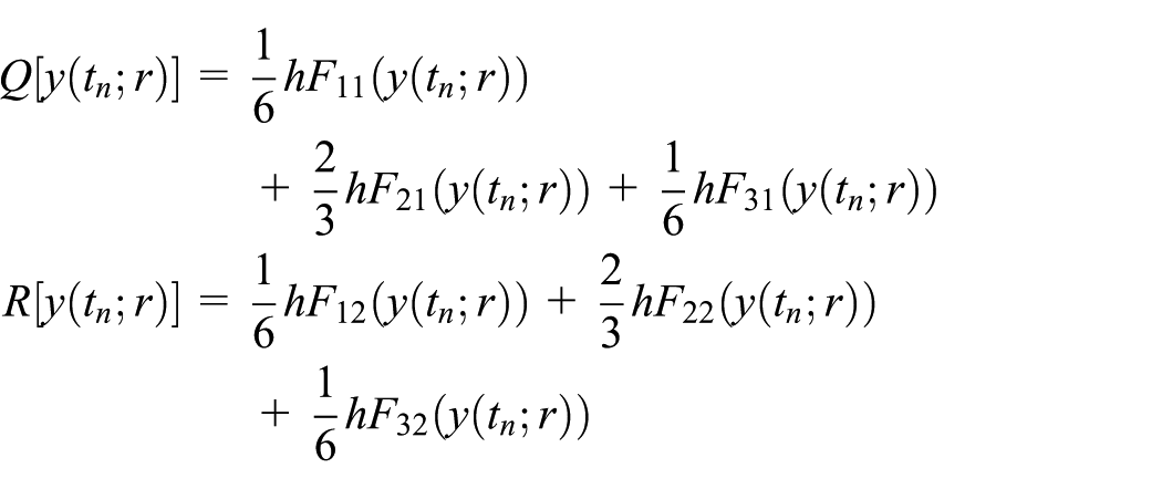
Based on equation (5), the fuzzy GLM of order 3 is given by

$$\begin{array}{c}{\left[y_1(t_{n+1};r)\right]}_i=\sum _{j=1}^{s=3}{b}_{\mathrm{ij}}h{F}_{j,1}(t_n,y(t_n;r))\hfill \\ +\sum _{j=1}^{r=2}{v}_{\mathrm{ij}}[y_1(t_n;r){]}_j,i=1,2,\dots ,r\hfill \end{array}$$

(9a)

$$\begin{array}{c}{\left[y_2(t_{n+1};r)\right]}_i\hfill \\ =\sum _{j=1}^{s=3}{b}_{\mathrm{ij}}h{F}_{j,2}(t_n,y(t_n;r))+\sum _{j=1}^{r=2}{v}_{\mathrm{ij}}[y_2(t_n;r){]}_j,\hfill \\ i=1,2,\dots ,r\hfill \end{array}$$

(9b)

where for type (i) differentiability is arranged as

$$\begin{array}{c}{F}_{11}(t_n,y(t_n;r))\hfill \\ =min\{f(t_n,u)|u\in [Y_{11}(t_n,y(t_n;r)),Y_{12}(t_n,y(t_n;r))]\}\hfill \\ F_{12}(t_n,y(t_n;r))\hfill \\ =max\{f(t_n,u)|u\in [Y_{11}(t_n,y(t_n;r)),Y_{12}(t_n,y(t_n;r))]\}\hfill \\ F_{21}(t_n,y(t_n;r))\hfill \\ =min\{f(t_n+c_{2}h,u)|u\in [Y_{21}(t_n,y(t_n;r)),Y_{22}(t_n,y(t_n;r))]\}\hfill \\ F_{22}(t_n,y(t_n;r))\hfill \\ =max\{f(t_n+c_{2}h,u)|u\in [Y_{21}(t_n,y(t_n;r)),Y_{22}(t_n,y(t_n;r))]\}\hfill \\ F_{31}(t_n,y(t_n;r))\hfill \\ =min\{f(t_n+c_{3}h,u)|u\in [Y_{31}(t_n,y(t_n;r)),Y_{32}(t_n,y(t_n;r))]\}\hfill \\ F_{32}(t_n,y(t_n;r))\hfill \\ =max\{f(t_n+c_{3}h,u)|u\in [Y_{31}(t_n,y(t_n;r)),Y_{32}(t_n,y(t_n;r))]\}\hfill \end{array}$$

(10)

while for type (ii) differentiability is arranged as

$$\begin{array}{c}{F}_{11}(t_n,y(t_n;r))\hfill \\ =max\{f(t_n,u)|u\in [Y_{11}(t_n,y(t_n;r)),Y_{12}(t_n,y(t_n;r))]\}\hfill \\ F_{12}(t_n,y(t_n;r))\hfill \\ =min\{f(t_n,u)|u\in [Y_{11}(t_n,y(t_n;r)),Y_{12}(t_n,y(t_n;r))]\}\hfill \\ F_{21}(t_n,y(t_n;r))\hfill \\ =max\{f(t_n+c_{2}h,u)|u\in [Y_{21}(t_n,y(t_n;r)),Y_{22}(t_n,y(t_n;r))]\}\hfill \\ F_{22}(t_n,y(t_n;r))\hfill \\ =min\{f(t_n+c_{2}h,u)|u\in [Y_{21}(t_n,y(t_n;r)),Y_{22}(t_n,y(t_n;r))]\}\hfill \\ F_{31}(t_n,y(t_n;r))\hfill \\ =max\{f(t_n+c_{3}h,u)|u\in [Y_{31}(t_n,y(t_n;r)),Y_{32}(t_n,y(t_n;r))]\}\hfill \\ F_{32}(t_n,y(t_n;r))\hfill \\ =min\{f(t_n+c_{3}h,u)|u\in [Y_{31}(t_n,y(t_n;r)),Y_{32}(t_n,y(t_n;r))]\}\hfill \end{array}$$

(11)

and

$$\begin{array}{c}{Y}_{11}(t_n,y(t_n;r))=\sum _{j=1}^{s=3}{a}_{1j}h{F}_{j,1}(t_n,y_1(t_n;r))+\sum _{j=1}^{r=2}{u}_{1j}[y_1(t_n;r){]}_j\hfill \\ Y_{12}(t_n,y(t_n;r))=\sum _{j=1}^{s=3}{a}_{1j}h{F}_{j,2}(t_n,y_2(t_n;r))+\sum _{j=1}^{r=2}{u}_{1j}[y_2(t_n;r){]}_j\hfill \\ Y_{21}(t_n,y(t_n;r))=\sum _{j=1}^{s=3}{a}_{2j}h{F}_{j,1}(t_n,y_1(t_n;r))+\sum _{j=1}^{r=2}{u}_{2j}[y_1(t_n;r){]}_j\hfill \\ Y_{22}(t_n,y(t_n;r))=\sum _{j=1}^{s=3}{a}_{2j}h{F}_{j,2}(t_n,y_2(t_n;r))+\sum _{j=1}^{r=2}{u}_{2j}[y_2(t_n;r){]}_j\hfill \\ Y_{31}(t_n,y(t_n;r))=\sum _{j=1}^{s=3}{a}_{2j}h{F}_{j,1}(t_n,y_1(t_n;r))+\sum _{j=1}^{r=2}{u}_{3j}[y_1(t_n;r){]}_j\hfill \\ Y_{32}(t_n,y(t_n;r))=\sum _{j=1}^{s=3}{a}_{2j}h{F}_{j,2}(t_n,y_2(t_n;r))+\sum _{j=1}^{r=2}{u}_{3j}[y_2(t_n;r){]}_j\hfill \end{array}$$

(12)

Consequence of theorem 1 in section “Introduction” leads to the conversion of fuzzy initial value problem into two parametric ordinary differential systems which consist of type (i) and type (ii) differentiabilities. Proof of this theorem was found in Nieto et al. ¹⁸ In this section, fuzzy GLM is developed for type (i) differentiability based on formulation (2) in definition 7. Meanwhile, fuzzy GLM for type (ii) differentiability is referred by formulation (3) in definition 7.

Convergence analysis

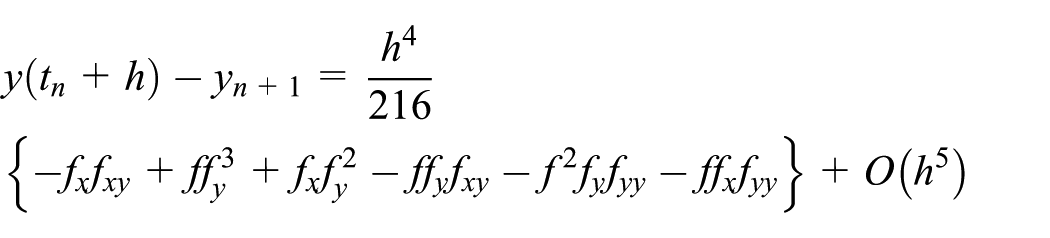
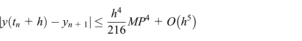
The local truncation error of third-order GLM using the Taylor series expansion related to the given coefficients in Table 5 is presented by

$$\begin{array}{c}T(t,h)=\frac{h^4}{216}\hfill \\ \{-f_x{f}_{\mathrm{xy}}+{\mathrm{ff}}_y^3+f_x{f}_y^2-f{f}_y{f}_{\mathrm{xy}}-f^2{f}_y{f}_{\mathrm{yy}}-f{f}_x{f}_{\mathrm{yy}}\}+O\left(h^5\right)\hfill \end{array}$$

(13)

From equation (13), the following lemma is applied.

Lemma 1

Let $f(y)$ belong to $C^4[a,b]$ and let its derivatives be bounded. ¹⁰ Also, assume that there exist P and M positive numbers, such that $|f(y)|<M,|d^{j}f/d{y}^j|<P^j/M^{j-1}$ , $j\le 4$ , then

$$y\left(t_n+h\right)-y_{n+1}=\frac{h^4}{216}\left\{-f_x{f}_{xy}+f{f}_y^3+f_x{f}_y^2-f{f}_y{f}_{xy}-f^2{f}_y{f}_{yy}-f{f}_x{f}_{yy}\right\}+O\left(h^5\right)$$

and

$$|y(t_n+h)-y_{n+1}|\le \frac{h^4}{216}M{P}^4+O\left(h^5\right)$$

Suppose the exact solutions $[\tilde{Y}(t){]}_r=[\widetilde{Y_1}(t;r),\widetilde{Y_2}(t;r)]$ is approximated by $[y(t){]}_r=[y_1(t;r),y_2(t;r)]$ . The solution is calculated by grid points $t_0<t_1<t_2\cdots <t_N=T$ where $h=(T-t_0)/N$ . Let $Q$ and $R$ be functions of $Q(t_n,y(t_n;r))$ and $R(t_n,y(t_n;r))$ , respectively. We have

$$\begin{array}{c}{y}_1(t_{n+1};r)=y_1(t_n;r)+Q[t_n,y(t_n;r)]\hfill \\ y_2(t_{n+1};r)=y_2(t_n;r)+R[t_n,y(t_n;r)]\hfill \end{array}$$

(14)

Also

$$\begin{array}{c}\widetilde{Y_1}(t_{n+1};r)=\widetilde{Y_1}(t_n;r)+Q[t_n,\tilde{Y}(t_n;r)]\hfill \\ \widetilde{Y_2}(t_{n+1};r)=\widetilde{Y_2}(t_n;r)+R[t_n,\tilde{Y}(t_n;r)]\hfill \end{array}$$

(15)

The domain where $Q$ and $R$ are defined in the region of $K$ is

$$K=\{(t,u,v)|t_0\le t\le T,-\infty <v<\infty ,-\infty <u<v\}$$

Then, we define the fuzzy third-order GLM as follows

$$\begin{array}{c}\multicolumn{1}{c}{Q\left[y(t_n;r)\right]=\frac{1}{6}h{F}_{11}\left(y(t_n;r)\right)}\\ +\frac{2}{3}h{F}_{21}\left(y(t_n;r)\right)+\frac{1}{6}h{F}_{31}\left(y(t_n;r)\right)\hfill \\ \multicolumn{1}{c}{R\left[y(t_n;r)\right]=\frac{1}{6}h{F}_{12}\left(y(t_n;r)\right)+\frac{2}{3}h{F}_{22}\left(y(t_n;r)\right)}\\ +\frac{1}{6}h{F}_{32}\left(y(t_n;r)\right)\hfill \end{array}$$

The following lemma and theorem are given to show the convergence of these approximates

$$\begin{array}{c}\underset{h\to 0}{lim}{y}_1(t;r)=\widetilde{Y_1}(t;r)\hfill \\ \underset{h\to 0}{lim}{y}_2(t;r)=\widetilde{Y_2}(t;r)\hfill \end{array}$$

Lemma 2

Let the sequence of numbers $\{W_n{\}}_{n=0}^N$ satisfy ^8,10

$$\left|W_{n+1}\right|\le A\left|W_n\right|+B,0\le n\le N-1$$

for some given positive constants $A$ and $B$ , then

$$\left|W_n\right|\le A^n\left|W_0\right|+B\frac{A^n-1}{A-1},0\le n\le N$$

Lemma 3

Let the sequence of numbers $\{W_n{\}}_{n=0}^N$ and $\{V_n{\}}_{n=0}^N$ satisfy ^8,10

$$\begin{array}{c}\left|W_{n+1}\right|\le \left|W_n\right|+A\max \{\left|W_n\right|,\left|V_n\right|\}+B\hfill \\ \left|V_{n+1}\right|\le \left|V_n\right|+A\max \{\left|W_n\right|,\left|V_n\right|\}+B\hfill \end{array}$$

for some given positive constants $A$ and $B$ and denote $U_n=\left|W_n\right|+\left|V_n\right|$ , $0\le n\le N$ . Then

$$U_n\le \overline{A}{U}_0+\overline{B}\frac{{\overline{A}}^n-1}{\overline{A}-1},\overline{A}=1+2A\mathrm{and}\overline{B}=2B$$

Theorem 3

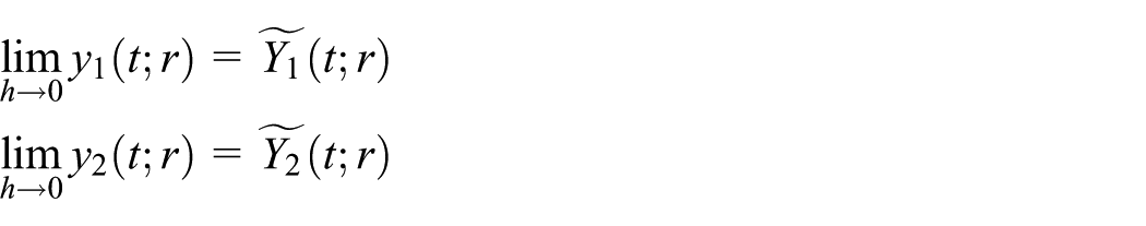
Let $Q(t,u,v)$ and $R(t,u,v)$ are in $C^{4}K$ and let the partial derivative of $Q$ and $R$ be bounded over $K$ , then for arbitrary fixed $r,0\le r\le 1$ , the approximate solution of equation (14) converge to the exact solutions $\widetilde{Y_1}(t;r)$ and $\widetilde{Y_2}(t;r)$ uniformly in $t$ . ¹⁰

Proof

It is sufficient to show

$$\begin{array}{c}\underset{h\to 0}{lim}{y}_1(t_N;r)=\widetilde{Y_1}(t_N;r)\hfill \\ \underset{h\to 0}{lim}{y}_2(t_N;r)=\widetilde{Y_2}(t_N;r)\hfill \end{array}$$

(16)

where $t_N=T$ . For $n=0,1,\dots ,N-1$ , using Taylor Theorem, we get

$$\begin{array}{c}\widetilde{Y_1}(t_{n+1};r)={\tilde{Y}}_1(t_n;r)+Q[\widetilde{Y_1}(t_n;r),\widetilde{Y_2}(t_n;r)]+\frac{h^4}{216}M{P}^4+O\left(h^5\right)\hfill \\ \widetilde{Y_2}(t_{n+1};r)={\tilde{Y}}_2(t_n;r)+R[\widetilde{Y_1}(t_n;r),\widetilde{Y_2}(t_n;r)]+\frac{h^4}{216}M{P}^4+O\left(h^5\right)\hfill \end{array}$$

(17)

denote

$$W_n=\widetilde{Y_1}(t_n;r)-y_1(t_n;r),V_n=\widetilde{Y_2}(t_n;r)-y_2(t_n;r)$$

Hence, from equations (14) and (17), we find

$$\begin{array}{c}{W}_{n+1}=W_n+Q[\widetilde{Y_1}(t_n;r),\widetilde{Y_2}(t_n;r)]\hfill \\ -Q[y_1(t_n;r),y_2(t_n;r)]+\frac{h^4}{216}M{P}^4+O\left(h^5\right)\hfill \\ V_{n+1}=V_n+Q[\widetilde{Y_1}(t_n;r),\widetilde{Y_2}(t_n;r)]\hfill \\ -Q[y_1(t_n;r),y_2(t_n;r)]+\frac{h^4}{216}M{P}^4+O\left(h^5\right)\hfill \end{array}$$

Then

$$\begin{array}{c}\left|W_{n+1}\right|\le \left|W_n\right|+2\mathrm{Lh}max\{\left|W_n\right|,\left|V_n\right|\}+\frac{h^4}{216}M{P}^4+O\left(h^5\right)\hfill \\ \left|V_{n+1}\right|\le \left|V_n\right|+2\mathrm{Lh}max\{\left|W_n\right|,\left|V_n\right|\}+\frac{h^4}{216}M{P}^4+O\left(h^5\right)\hfill \end{array}$$

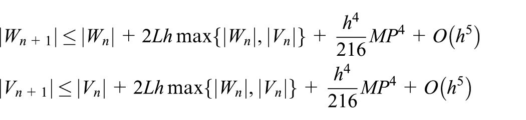
For $t\in [0,T]$ and $L>0$ is a bound for partial derivatives of $Q$ and $R$ . Thus, by lemma 2

$$\begin{array}{c}\left|W_n\right|\le {(1+4\mathrm{Lh})}^n\left|U_0\right|+(\frac{h^4}{108}M{P}^4+O\left(h^5\right))\hfill \\ \frac{{(1+4\mathrm{Lh})}^n-1}{4\mathrm{Lh}}\hfill \\ \left|V_n\right|\le {(1+4\mathrm{Lh})}^n\left|U_0\right|+(\frac{h^4}{108}M{P}^4+O\left(h^5\right))\hfill \\ \frac{{(1+4\mathrm{Lh})}^n-1}{4\mathrm{Lh}}\hfill \end{array}$$

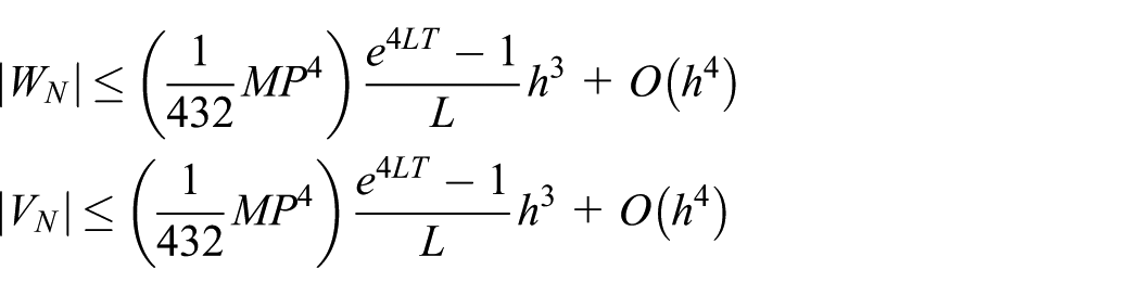
where $\left|U_0\right|=\left|W_0\right|+\left|V_0\right|$ . In particular

$$\begin{array}{c}\left|W_N\right|\le {(1+4\mathrm{Lh})}^n\left|U_0\right|+(\frac{h^3}{432}M{P}^4+O\left(h^4\right))\hfill \\ \frac{{(1+4\mathrm{Lh})}^n-1}{L}\hfill \\ \left|V_N\right|\le {(1+4\mathrm{Lh})}^n\left|U_0\right|+(\frac{h^3}{432}M{P}^4+O\left(h^4\right))\hfill \\ \frac{{(1+4\mathrm{Lh})}^n-1}{L}\hfill \end{array}$$

since $W_0=V_0=0$ , we obtain

$$\begin{array}{c}\left|W_N\right|\le \left(\frac{1}{432}M{P}^4\right)\frac{e^{4\mathrm{LT}}-1}{L}{h}^3+O\left(h^4\right)\hfill \\ \left|V_N\right|\le \left(\frac{1}{432}M{P}^4\right)\frac{e^{4\mathrm{LT}}-1}{L}{h}^3+O\left(h^4\right)\hfill \end{array}$$

and if $h\to 0$ , we get $W_N\to 0,V_N\to 0$ which completes the proof.

Numerical results

To show the efficiency of derived third-order fuzzy GLM, the method is numerically tested on three test problems. All problems are tested based on type (i) differentiability using formulation (15) in section “Third-order fuzzy GLM.” The accuracy of the method in terms of global error is estimated by the expressions $E_1(t;r)=|y_1(t;r)-{\tilde{Y}}_1(t;r)|$ and $E_2(t;r)=|y_2(t;r)-{\tilde{Y}}_2(t;r)|$ . The numerical results are compared with existing Euler method, ¹⁸ Runge–Kutta method of order 4, ⁶ trapezoidal method (TM), ¹² and ANN method. ¹¹ Below is the list of notation used in the tabulated results:

• r r-level set of fuzzy number

• $y_1(t;r)$   lower bound of approximate solution

• $y_2(t;r)$   upper bound of approximate solution

• $\widetilde{Y_1}(t;r)$  lower bound of exact solution

• $\widetilde{Y_2}(t;r)$  upper bound of exact solution

• GLM  GLM of order 3 derived in this article

• Euler  Euler method derived by Nieto et al. ¹⁸

• RK  Runge–Kutta method of order 4 derived by Ghanaie and Moghadam ⁶

• TM  trapezoidal method derived by Ivaz et al. ¹²

• ANN  artificial neural network method derived by Effati and Pakdaman ¹¹

Problem 1

Consider the nuclear decay equation ¹⁸

$$y\prime \left(t\right)=-\lambda \odot y\left(t\right),y\left(0\right)=y_0$$

Let $\lambda =1$ , $t=[0,0.1]$ , and $y_0=[r-1,1-r]$ .

If $y(t)$ is $(\mathrm{i})$ differentiable, then the exact solution is given as

$${\tilde{Y}}_1(t;r)=(r-1)e^t,{\tilde{Y}}_2(t;r)=(1-r)e^t$$

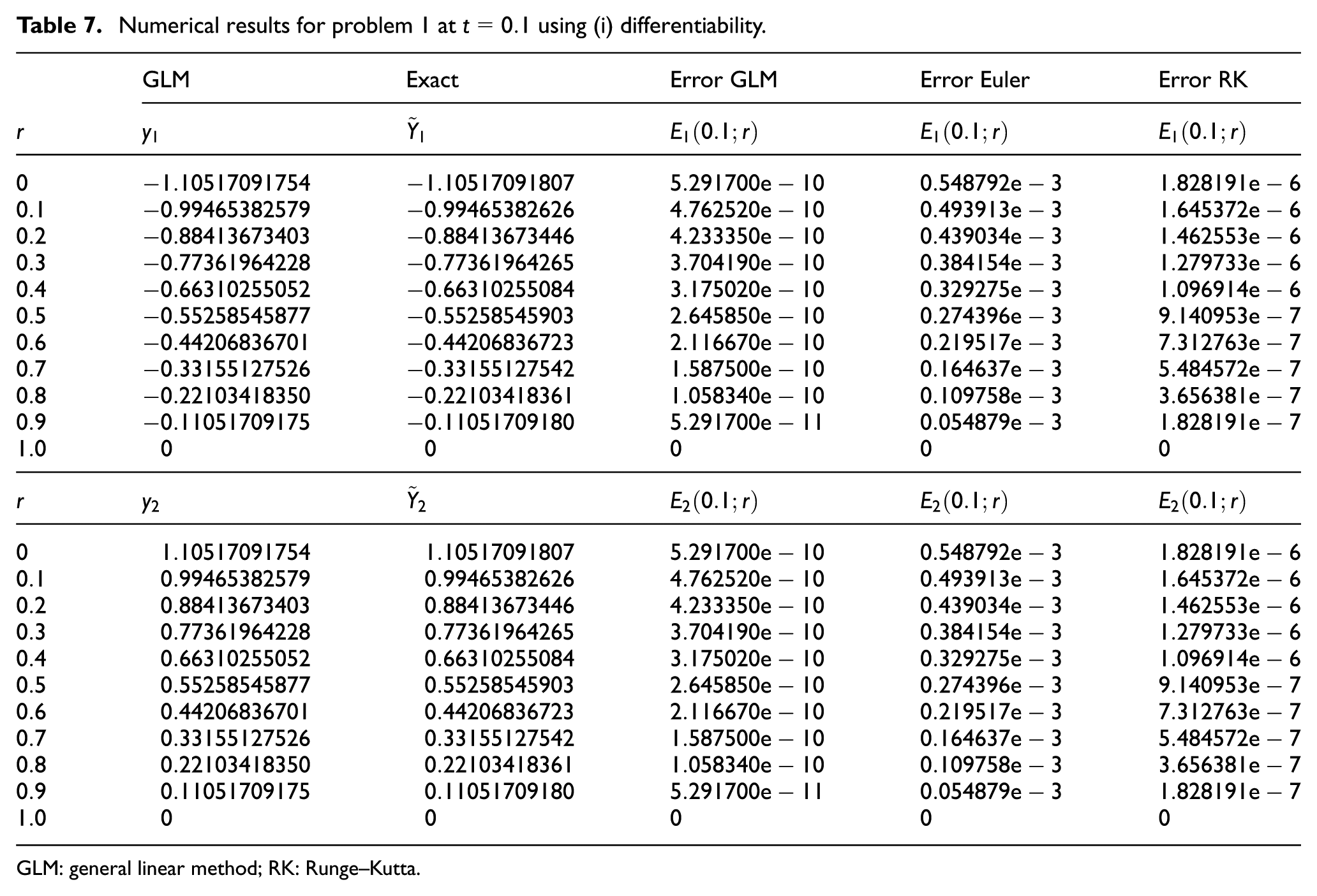
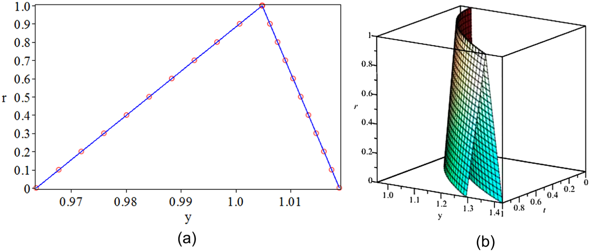
Based on formulation (2), the approximated solutions using third-order GLM at $t=0.1$ and $N=10$ subintervals are compared with Euler method and Runge–Kutta method and are shown in Table 7. Figure 1 shows the plotted graph of GLM with the exact solution.

Table 7.

Numerical results for problem 1 at $t=0.1$ using (i) differentiability.

	GLM	Exact	Error GLM	Error Euler	Error RK
$r$	$y_1$	${\tilde{Y}}_1$	$E_1(0.1;r)$	$E_1(0.1;r)$	$E_1(0.1;r)$
$0$	$-1.10517091754$	$-1.10517091807$	$5.291700\mathrm{e}-10$	$0.548792\mathrm{e}-3$	$1.828191\mathrm{e}-6$
$0.1$	$-0.99465382579$	$-0.99465382626$	$4.762520\mathrm{e}-10$	$0.493913\mathrm{e}-3$	$1.645372\mathrm{e}-6$
$0.2$	$-0.88413673403$	$-0.88413673446$	$4.233350\mathrm{e}-10$	$0.439034\mathrm{e}-3$	$1.462553\mathrm{e}-6$
$0.3$	$-0.77361964228$	$-0.77361964265$	$3.704190\mathrm{e}-10$	$0.384154\mathrm{e}-3$	$1.279733\mathrm{e}-6$
$0.4$	$-0.66310255052$	$-0.66310255084$	$3.175020\mathrm{e}-10$	$0.329275\mathrm{e}-3$	$1.096914\mathrm{e}-6$
$0.5$	$-0.55258545877$	$-0.55258545903$	$2.645850\mathrm{e}-10$	$0.274396\mathrm{e}-3$	$9.140953\mathrm{e}-7$
$0.6$	$-0.44206836701$	$-0.44206836723$	$2.116670\mathrm{e}-10$	$0.219517\mathrm{e}-3$	$7.312763\mathrm{e}-7$
$0.7$	$-0.33155127526$	$-0.33155127542$	$1.587500\mathrm{e}-10$	$0.164637\mathrm{e}-3$	$5.484572\mathrm{e}-7$
$0.8$	$-0.22103418350$	$-0.22103418361$	$1.058340\mathrm{e}-10$	$0.109758\mathrm{e}-3$	$3.656381\mathrm{e}-7$
$0.9$	$-0.11051709175$	$-0.11051709180$	$5.291700\mathrm{e}-11$	$0.054879\mathrm{e}-3$	$1.828191\mathrm{e}-7$
$1.0$	$0$	$0$	$0$	$0$	$0$
$r$	$y_2$	${\tilde{Y}}_2$	$E_2(0.1;r)$	$E_2(0.1;r)$	$E_2(0.1;r)$
$0$	$1.10517091754$	$1.10517091807$	$5.291700\mathrm{e}-10$	$0.548792\mathrm{e}-3$	$1.828191\mathrm{e}-6$
$0.1$	$0.99465382579$	$0.99465382626$	$4.762520\mathrm{e}-10$	$0.493913\mathrm{e}-3$	$1.645372\mathrm{e}-6$
$0.2$	$0.88413673403$	$0.88413673446$	$4.233350\mathrm{e}-10$	$0.439034\mathrm{e}-3$	$1.462553\mathrm{e}-6$
$0.3$	$0.77361964228$	$0.77361964265$	$3.704190\mathrm{e}-10$	$0.384154\mathrm{e}-3$	$1.279733\mathrm{e}-6$
$0.4$	$0.66310255052$	$0.66310255084$	$3.175020\mathrm{e}-10$	$0.329275\mathrm{e}-3$	$1.096914\mathrm{e}-6$
$0.5$	$0.55258545877$	$0.55258545903$	$2.645850\mathrm{e}-10$	$0.274396\mathrm{e}-3$	$9.140953\mathrm{e}-7$
$0.6$	$0.44206836701$	$0.44206836723$	$2.116670\mathrm{e}-10$	$0.219517\mathrm{e}-3$	$7.312763\mathrm{e}-7$
$0.7$	$0.33155127526$	$0.33155127542$	$1.587500\mathrm{e}-10$	$0.164637\mathrm{e}-3$	$5.484572\mathrm{e}-7$
$0.8$	$0.22103418350$	$0.22103418361$	$1.058340\mathrm{e}-10$	$0.109758\mathrm{e}-3$	$3.656381\mathrm{e}-7$
$0.9$	$0.11051709175$	$0.11051709180$	$5.291700\mathrm{e}-11$	$0.054879\mathrm{e}-3$	$1.828191\mathrm{e}-7$
$1.0$	$0$	$0$	$0$	$0$	$0$

GLM: general linear method; RK: Runge–Kutta.

Figure 1.

(a) Exact (solid line) and GLM (circle) points at $t=0.1$ using (i) differentiability and (b) 3D plot for problem 1.

Problem 2

Use the initial values in problem 1, let $\lambda =1$ , $t=[0,1]$ , ¹² and $y_0=[0.96+0.04r,1.01-0.01r]$ . The exact solution is given by

$$\begin{array}{c}{\tilde{Y}}_1(t;r)=(0.985+0.015r)e^{-t}-(1-r)0.025e^t\hfill \\ {\tilde{Y}}_2(t;r)=(0.985+0.015r)e^{-t}+(1-r)0.025e^t\hfill \end{array}$$

The graphs of exact solutions and approximated solutions and three-dimensional (3D) plot for problem 2 are shown in Figure 2. Table 8 shows that the numerical solutions of GLM are compared with the TM.

Figure 2.

(a) Exact (solid line) and GLM (circle) points at $t=0.1$ and (b) 3D plot for problem 2.

Table 8.

Numerical results for problem 2 at $t=0.1$ .

	GLM	TM	Exact	Error GLM	Error TM
$r$	$y_1$	$y_1$	${\tilde{Y}}_1$	$E_1(0.1;r)$	$E_1(0.1;r)$
$0$	$0.8636353$	$0.8636348$	$0.8636355$	$2.339370\mathrm{e}-7$	$8.0\mathrm{e}-7$
$0.1$	$0.8677555$	$0.8677550$	$0.8677557$	$2.359889\mathrm{e}-7$	$8.0\mathrm{e}-7$
$0.2$	$0.8718757$	$0.8718752$	$0.8718759$	$2.380407\mathrm{e}-7$	$7.0\mathrm{e}-7$
$0.3$	$0.8759958$	$0.8759954$	$0.8759961$	$2.400926\mathrm{e}-7$	$7.0\mathrm{e}-7$
$0.4$	$0.8801160$	$0.8801156$	$0.8801163$	$2.421445\mathrm{e}-7$	$7.0\mathrm{e}-7$
$0.5$	$0.8842362$	$0.8842357$	$0.8842365$	$2.441963\mathrm{e}-7$	$8.0\mathrm{e}-7$
$0.6$	$0.8883564$	$0.8883559$	$0.8883566$	$2.462482\mathrm{e}-7$	$8.0\mathrm{e}-7$
$0.7$	$0.8924766$	$0.8924761$	$0.8924768$	$2.483001\mathrm{e}-7$	$8.0\mathrm{e}-7$
$0.8$	$0.8965968$	$0.8965963$	$0.8965970$	$2.503520\mathrm{e}-7$	$7.0\mathrm{e}-7$
$0.9$	$0.9007169$	$0.9007165$	$0.9007172$	$2.524038\mathrm{e}-7$	$8.0\mathrm{e}-7$
$1.0$	$0.9048371$	$0.9048367$	$0.9048374$	$2.544557\mathrm{e}-7$	$7.0\mathrm{e}-7$
$\mathit{r}$	${\mathit{y}}_2$	${\mathit{y}}_2$	${\tilde{\mathit{Y}}}_2$	${\mathit{E}}_2(0.1;\mathit{r})$	${\mathit{E}}_2(0.1;\mathit{r})$
$0$	$0.9188938$	$0.9188934$	$0.9188941$	$2.673408\mathrm{e}-7$	$7.0\mathrm{e}-7$
$0.1$	$0.9174881$	$0.9174877$	$0.9174884$	$2.660523\mathrm{e}-7$	$8.0\mathrm{e}-7$
$0.2$	$0.9160825$	$0.9160821$	$0.9160827$	$2.647638\mathrm{e}-7$	$7.0\mathrm{e}-7$
$0.3$	$0.9146768$	$0.9146764$	$0.9146771$	$2.634752\mathrm{e}-7$	$7.0\mathrm{e}-7$
$0.4$	$0.9132711$	$0.9132707$	$0.9132714$	$2.621867\mathrm{e}-7$	$7.0\mathrm{e}-7$
$0.5$	$0.9118655$	$0.9118651$	$0.9118657$	$2.608982\mathrm{e}-7$	$7.0\mathrm{e}-7$
$0.6$	$0.9104598$	$0.9104593$	$0.9104601$	$2.596097\mathrm{e}-7$	$8.0\mathrm{e}-7$
$0.7$	$0.9090541$	$0.9090537$	$0.9090544$	$2.583212\mathrm{e}-7$	$8.0\mathrm{e}-7$
$0.8$	$0.9076485$	$0.9076480$	$0.9076487$	$2.570327\mathrm{e}-7$	$7.0\mathrm{e}-7$
$0.9$	$0.9062428$	$0.9062423$	$0.9062430$	$2.557442\mathrm{e}-7$	$8.0\mathrm{e}-7$
$1.0$	$0.9048371$	$0.9048367$	$0.9048374$	$2.544557\mathrm{e}-7$	$7.0\mathrm{e}-7$

GLM: general linear method; TM: trapezoidal method.

Problem 3

$$y^{\prime }(t)=-y(t)+t+1,y(0)=y_0$$

Let $t=[0,1]$ and $y_0=[0.96+0.04r,1.01-001r]$ . ¹¹ The exact solution is given as

$$\begin{array}{c}{\tilde{Y}}_1(t;r)=t+(0.985+0.015r)e^{-t}-(1-r)0.025e^t,\hfill \\ {\tilde{Y}}_2(t;r)=t+(0.985+0.015r)e^{-t}+(1-r)0.025e^t.\hfill \end{array}$$

We compared the GLM with the TM and ANN method at $t=0.1$ , $N=10$ , and the results are given in Table 9. Figure 1 shows the plotted graph of GLM with the exact solution and 3D plot for problem 3.

Table 9.

Numerical results for problem 3 at $t=0.1$ .

	GLM	Exact	Error GLM	Error TM	Error ANN
$\mathit{r}$	${\mathit{y}}_1$	${\tilde{\mathit{Y}}}_1$	${\mathit{E}}_1(0.1;\mathit{r})$	${\mathit{E}}_1(0.1;\mathit{r})$	${\mathit{E}}_1(0.1;\mathit{r})$
$0$	$0.9636353$	$0.9636356$	$2.339370\mathrm{e}-7$	$8.0\mathrm{e}-7$	$5.067853\mathrm{e}-5$
$0.1$	$0.9677555$	$0.9677558$	$2.359889\mathrm{e}-7$	$8.0\mathrm{e}-7$	$3.873561\mathrm{e}-5$
$0.2$	$0.9718757$	$0.9718759$	$2.380407\mathrm{e}-7$	$8.0\mathrm{e}-7$	$2.067133\mathrm{e}-5$
$0.3$	$0.9759959$	$0.9759961$	$2.400926\mathrm{e}-7$	$7.0\mathrm{e}-7$	$6.021995\mathrm{e}-5$
$0.4$	$0.9801161$	$0.9801163$	$2.421445\mathrm{e}-7$	$8.0\mathrm{e}-7$	$7.410150\mathrm{e}-6$
$0.5$	$0.9842363$	$0.9842365$	$2.441963\mathrm{e}-7$	$7.0\mathrm{e}-7$	$0.6225859-5$
$0.6$	$0.9883564$	$0.9883567$	$2.462482\mathrm{e}-7$	$8.0\mathrm{e}-7$	$3.472099\mathrm{e}-5$
$0.7$	$0.9924766$	$0.9924769$	$2.483001\mathrm{e}-7$	$8.0\mathrm{e}-7$	$4.320305\mathrm{e}-5$
$0.8$	$0.9965968$	$0.9965970$	$2.503520\mathrm{e}-7$	$8.0\mathrm{e}-7$	$1.614909\mathrm{e}-5$
$0.9$	$1.0007170$	$1.0007172$	$2.524038\mathrm{e}-7$	$9.0\mathrm{e}-7$	$1.253534\mathrm{e}-5$
$1.0$	$1.0048372$	$1.0048374$	$2.544557\mathrm{e}-7$	$7.0\mathrm{e}-7$	$2.142460\mathrm{e}-6$
$\mathit{r}$	${\mathit{y}}_2$	${\tilde{\mathit{Y}}}_2$	${\mathit{E}}_2(0.1;\mathit{r})$	${\mathit{E}}_2(0.1;\mathit{r})$	${\mathit{E}}_2(0.1;\mathit{r})$
$0$	$1.0188939$	$1.0188941$	$2.673408\mathrm{e}-7$	$7.0\mathrm{e}-7$	$3.753089\mathrm{e}-5$
$0.1$	$1.0174882$	$1.0174885$	$2.660523\mathrm{e}-7$	$7.0\mathrm{e}-7$	$4.153197\mathrm{e}-5$
$0.2$	$1.0160825$	$1.0160828$	$2.647638\mathrm{e}-7$	$8.0\mathrm{e}-7$	$7.614799\mathrm{e}-6$
$0.3$	$1.0146768$	$1.0146771$	$2.634753\mathrm{e}-7$	$9.0\mathrm{e}-7$	$3.922612\mathrm{e}-5$
$0.4$	$1.0132712$	$1.0132714$	$2.621868\mathrm{e}-7$	$8.0\mathrm{e}-7$	$4.092031\mathrm{e}-5$
$0.5$	$1.0118655$	$1.0118658$	$2.608982\mathrm{e}-7$	$7.0\mathrm{e}-7$	$3.571873\mathrm{e}-5$ .
$0.6$	$1.0104698$	$1.0104601$	$2.596097\mathrm{e}-7$	$8.0\mathrm{e}-7$	$2.494235\mathrm{e}-5$
$0.7$	$1.0090542$	$1.0090544$	$2.583212\mathrm{e}-7$	$7.0\mathrm{e}-7$	$4.355865\mathrm{e}-5$
$0.8$	$1.0076485$	$1.0076488$	$2.570327\mathrm{e}-7$	$7.0\mathrm{e}-7$	$2.703282\mathrm{e}-5$
$0.9$	$1.0062428$	$1.0062431$	$2.557442\mathrm{e}-7$	$7.0\mathrm{e}-7$	$3.883441\mathrm{e}-5$
$1.0$	$1.0048372$	$1.0048374$	$2.544557\mathrm{e}-7$	$7.0\mathrm{e}-7$	$1.924814\mathrm{e}-5$

GLM: general linear method; ANN: artificial neural network.

Comparison and discussion

From problem 1, the results given in Table 7 showed that the GLM with error ${10}^{-10}$ performed higher accuracy than the Euler method with error of ${10}^{-3}$ and Runge–Kutta method with error ${10}^{-7}$ . Graph comparison between approximated solutions by GLM and exact solutions can be seen in Figure 1. In problem 2, the numerical result of GLM is compared with the TM as shown in Table 8, and it is obvious that GLM produced error of ${10}^{-7}$ , while its error is slightly smaller than error obtained by TM. In Figure 2, the graph indicates that the approximated solutions of GLM are close to the exact solutions. In problem 3, from Table 9, it can be seen that GLM by achieving the error accuracy of ${10}^{-7}$ is the most accurate method with the smaller error compared to the ANN with the error of ${10}^{-5}$ and TM with the error of ${10}^{-7}$ . The graphical representation of approximated solutions and exact solutions is shown in Figure 3. The 3D plots of solution for three tested problems are shown.

Figure 3.

(a) Exact (solid line) and GLM (circle) points at $t=0.1$ and (b) 3D plot for problem 3.

Conclusion

In conclusion, in this article, GLM of order 3 based on the rooted trees and B-series is developed. The rooted trees act as a powerful tool in extracting the order conditions of a method. We had given out the order conditions as well as a new set of coefficients of GLM. Then, we constructed the fuzzy GLM using the concept of generalized Hukuhara differentiability. The new method applied with the derived coefficients of GLM of order 3 into the fuzzy differential test problems. The numerical results compared with the existing numerical methods showed that the fuzzy GLM is an efficient method for solving FDEs.