Performance analysis of a complex queueing system with vacations in random environment

Abstract

This article studies a complex queueing system with vacations in a multi-phase random environment. When the system is in operative phase $i$ , $i=1,2,\dots ,n$ , customers are served one by one. Whenever the system becomes empty at a service completion instant, the server starts a vacation, causing the system to move to vacation phase. When a vacation ends, if the system is empty, another begins. Otherwise, the system moves from the vacation phase to some operative phase $i$ with probability $q_i$ , $i=1,2,\dots ,n$ . Using the method of probability generating function, we obtain the distribution for the steady-state queue length at arbitrary epoch. We also derive the distributions for the stationary sojourn time and the length of the server’s working time in a service cycle, respectively. Finally, we present some special cases and numerical examples.

Introduction

Due to the important applications in various fields, such as production managing, computer systems, and communication networks, the vacation queues have been largely investigated in the past three decades. In 1986, Doshi ¹ wrote an excellent survey on vacation models. Since then, a large number of papers on vacation models have appeared, and many kinds of vacation policies have been presented. We give a few examples. Servi and Finn ² first introduced working vacation policy in an $M/M/1$ queueing system, where the server provides service at a lower speed rather than completely stopping service during the vacation period. Later, Li and Tian ³ studied a $\mathrm{GI}/\mathrm{Geo}/1$ queue with working vacations and introduced a new policy: vacation interruption in their paper. Under such a policy, the server can come back to the normal service rate no matter whether the vacation ends. And Gao and Liu ⁴ presented an $M/G/1$ queue with single working vacation and vacation interruption under Bernoulli schedule. In this model, a customer is served at a lower service rate in the working vacation, and if there are customers in the queue at the instant of a service completion, the server resumes a normal busy period with probability $p$ or continues the vacation with probability $1-p$ . Recently, Vijaya Laxmi and Jyothsna ⁵ investigated an $M/M/1$ queue with working vacations and Bernoulli schedule vacation interruption wherein the customers may be impatient. That is, during a working vacation, customers may renege due to impatience. Ye and Liu ⁶ considered an M/M/1 queue with two vacation policies which comprise single working vacation and multiple vacations. For more comprehensive and excellent study on vacation models, the readers may refer to some researchers’ works such as Takagi, ⁷ Tian and Zhang, ⁸ and Ke et al. ⁹

The emergence of queueing system operating in random environment has attracted much attention due to its important applications in many fields, such as manufacturing system, transportation system, and financial system. An $M/M/1$ queue in a two-phase random environment has been studied by Yechiali and Naor, ¹⁰ Yechiali, ¹¹ Neuts, ¹² Kella and Whitt, ¹³ and others, where the arrival and service levels may vary in different phase. And some researchers discussed the $M/G/1$ queue in a two-phase random environment, for example, Neuts, ¹⁴ Boxma and Kurkova, ¹⁵ and Huang and Lee. ¹⁶ Falin ¹⁷ studied the $M/M/\infty$ queue with arrival and service rate depending on the state of an auxiliary semi-Markov process and obtained the mean number of customers in the system. Blom et al. ¹⁸ analyzed several aspects of the Markov-modulated infinite-server queue and derived some interesting results, such as some limit property. Baykal-Gursoy et al. ¹⁹ analyzed the vehicular traffic flow interrupted by incidents using $M/M/c$ queueing models. Cordeiro and Kharoufeh ²⁰ studied an $M/M/1$ retrial queue with an unreliable server whose arrival, service, failure, repair, and retrial rates are all modulated by an exogenous random environment. Kim and Kim ²¹ investigated a single server queue in which the service rate varied according to the underlying continuous time Markov process with finite states. Paz and Yechiali ²² studied an $M/M/1$ queue in a multi-phase random environment where the system suffered a disastrous failure. Jiang et al. ²³ extended ²² to an $M/G/1$ queueing system.

The $M/M/1$ queue with vacation and $M/M/1$ queue in random environment have been investigated extensively. But, to the best of our knowledge, the queueing system with vacations operating in random environment, which will be discussed in this article, has not been studied. But in fact, such a queueing system has many significant applications. For example, in a production system, the server usually has a vacation period when there is no workload to be processed. If on return from a vacation, the server finds one or more customers waiting, he or she goes on serving until the system becomes empty. But the service rate may change. The new service rate may depend on the arrival rate, environmental conditions, and operator experience. The above situation can be modeled by the queueing system with vacations operating in random environment. Also, the queueing system we discuss can be applied to performance evaluation of multibody systems. In general, complex mechanical systems (multibody systems) in many engineering fields, such as weapons, vehicles, and precision machineries, can be thought of as service systems. For example, a manufacturing facility used for producing customer-specified orders can be considered to be a server. The server takes vacations when there are no customer backorders. When returning from vacations, the server may have a new service intensity because of the different environmental conditions, such as different order quantity and different operator experience. In this situation, it is likely that the performance of the manufacturing facility can be evaluated by the queueing system we consider.

The rest of this article is organized as follows. Section “Model description” provides the model description. Section “Steady-state distribution” is devoted to obtain the probability generating function (PGF) of the steady-state queue length distributions at an arbitrary epoch. In section “Performance measure,” various performance measures, such as average queue length, average sojourn time, and the average length of working time in a service cycle, are calculated. Section “Special case” presents two special cases. Section “Numerical results” gives some numerical results and section “Conclusion” concludes the article.

Model description

We consider an $M/M/1$ type queueing system with vacations operating in a multi-phase random environment. When the system is in operative phase $i$ , $i=1,2,\dots ,n$ , customers arrive according to a Poisson process of rate ${\lambda }_i$ , and the service times of successive customers are independent and identically distributed random variables with exponential distribution with rate ${\mu }_i$ . Customers are served one by one according to the discipline of first-come first-served (FCFS). Whenever the system becomes empty at a service completion instant, the server starts a vacation, causing the system to move to a vacation phase $0$ . The vacation time $V$ is exponentially distributed with rate $\theta$ . In phase $0$ , the Poisson arrival rate is ${\lambda }_0$ , and the server does not serve customers. When a vacation ends, if the system is empty, another begins. Otherwise, the system jumps from the vacation phase $0$ to some operative phase $i$ with probability $q_i$ , $i=1,2,\dots ,n$ , where $q_i>0$ , $\sum _{i=1}^n{q}_i=1$ . Note that there are no direct jumps among the operative phases. That is, if the system is in phase $i$ , $i=1,2,\dots ,n$ , it must move to phase 0 when the system is empty. It stays in phase $0$ until there are customers in the system when a vacation ends, only then, can the system jump back to one of the operative phase $i$ , $i=1,2,\dots ,n$ .

We represent the state of the system at time $t$ by a pair $(L(t),J(t))$ , where $L(t)$ records the number of customers in the system and $J(t)$ denotes the phase in which the system operates. It is obvious that the process $\{(L(t),J(t)):t\ge 0\}$ is a continuous time Markov chain with state space $S=\{((m,0),m\ge 0)\cup ((m,i),m\ge 1,i=1,2,\dots ,n)\}$ and its transition rate diagram is shown in Figure 1.

Figure 1.

State transition rate diagram of $\{(L(t),J(t))\}$ .

Steady-state distribution

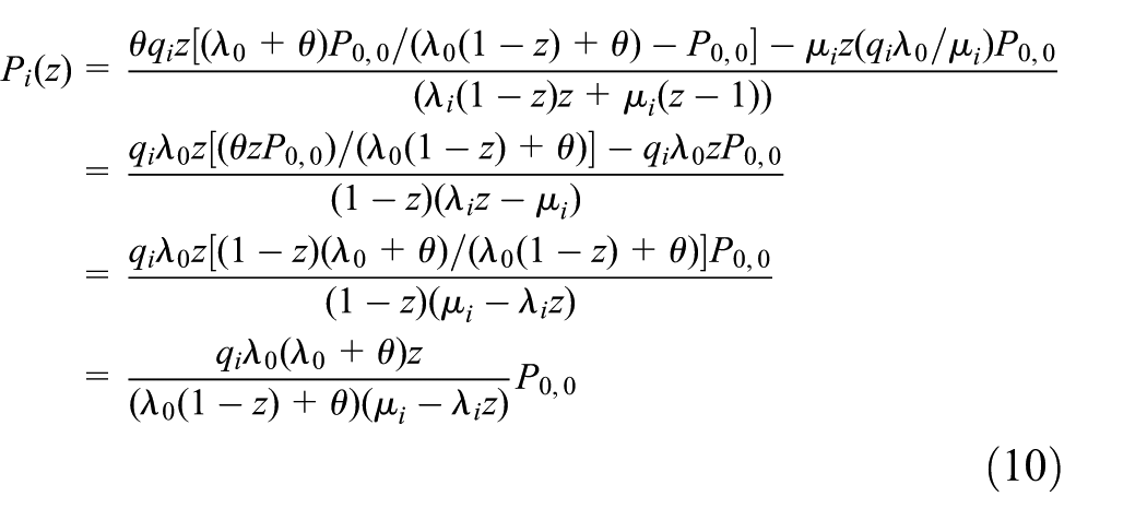
In operative phase $i$ , $i=1,2,\dots ,n$ , it is readily seen that the system acts as the classical M/M/1 queue with Poisson arrival rate ${\lambda }_i$ and service rate ${\mu }_i$ . So as long as ${\rho }_i={\lambda }_i/{\mu }_i<1$ , $i=1,2,\dots ,n$ , the system is stable. Moreover, if ${\rho }_i\ge 1$ for a certain $i$ , when the system moves to phase $i$ , the system will not be stable. Hence, ${\rho }_i={\lambda }_i/{\mu }_i<1$ , $i=1,2,\dots ,n$ , is the necessary and sufficient condition for the stability of the system we consider.

Assume that the above stability condition is fulfilled. Next, we analyze the steady-state distribution of the system.

We first define

$$\begin{array}{c}\hfill P_{m,0}=\underset{t\to \infty }{lim}P\{L(t)=m,J(t)=0\}\mathrm{for}m\ge 0\hfill \\ \multicolumn{1}{c}{P_{m,i}=\underset{t\to \infty }{lim}P\{L(t)=m,J(t)=i\}\mathrm{for}m\ge 1,\mathrm{and}i=1,2,\dots ,n}\end{array}$$

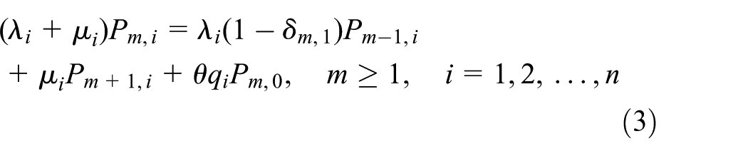
The system’s steady-state balance equations are presented below

$${\lambda }_0{P}_{0,0}=\sum _{i=1}^n{\mu }_i{P}_{1,i}$$

(1)

$$({\lambda }_0+\theta )P_{m,0}={\lambda }_0{P}_{m-1,0},m\ge 1$$

(2)

$$\begin{array}{l}({\lambda }_i+{\mu }_i)P_{m,i}={\lambda }_i(1-{\delta }_{m,1})P_{m-1,i}\\ +{\mu }_i{P}_{m+1,i}+\theta q_i{P}_{m,0},m\ge 1,i=1,2,\dots ,n\end{array}$$

(3)

where ${\delta }_{m,1}$ is the Kronecker symbol.

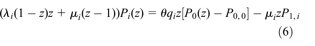
We will use the method of PGF to solve the above balance equations, so we define the partial PGFs as follows

$$P_0(z)=\sum _{m=0}^{\infty }{P}_{m,0}{z}^m$$

$$P_i(z)=\sum _{m=1}^{\infty }{P}_{m,i}{z}^m,i=1,2,\dots ,n$$

From equation (2), we have

$$P_{m,0}={\left(\frac{{\lambda }_0}{{\lambda }_0+\theta }\right)}^m{P}_{0,0},m\ge 1$$

(4)

Using equation (4), we get

$$\begin{array}{l}{P}_0(z)={\displaystyle \sum _{m=0}^{\infty }{P}_{m,0}}{z}^m={\displaystyle \sum _{m=0}^{\infty }{\left(\frac{{\lambda }_0}{{\lambda }_0+\theta }\right)}^m}{z}^m\\ P_{0,0}=\frac{{\lambda }_0+\theta }{{\lambda }_0(1-z)+\theta }{P}_{0,0}\end{array}$$

(5)

Multiplying equation (3) by $z^m$ and summing up these equations, after some algebra calculations, we have

$$({\lambda }_i(1-z)z+{\mu }_i(z-1))P_i(z)=\theta q_{i}z[P_0(z)-P_{0,0}]-{\mu }_{i}z{P}_{1,i}$$

(6)

Setting $z=1$ in equation (6), it follows that

$$P_{1,i}=\frac{\theta q_i[P_0(1)-P_{0,0}]}{{\mu }_i}$$

(7)

And by equation (5), we have

$$P_0(1)=\frac{{\lambda }_0+\theta }{\theta }{P}_{0,0}$$

(8)

Substituting equation (8) into equation (7), we get

$$P_{1,i}=\frac{q_i{\lambda }_0}{{\mu }_i}{P}_{0,0}$$

(9)

Substituting equations (5) and (9) into equation (6), we obtain

$$\begin{array}{cc}\multicolumn{1}{c}{P_i(z)}& =\frac{\theta q_{i}z[({\lambda }_0+\theta )P_{0,0}/({\lambda }_0(1-z)+\theta )-P_{0,0}]-{\mu }_{i}z(q_i{\lambda }_0/{\mu }_i)P_{0,0}}{({\lambda }_i(1-z)z+{\mu }_i(z-1))}\hfill \\ \multicolumn{1}{c}{}& =\frac{q_i{\lambda }_{0}z[(\theta z{P}_{0,0})/({\lambda }_0(1-z)+\theta )]-q_i{\lambda }_{0}z{P}_{0,0}}{(1-z)({\lambda }_{i}z-{\mu }_i)}\hfill \\ \multicolumn{1}{c}{}& =\frac{q_i{\lambda }_{0}z[(1-z)({\lambda }_0+\theta )/({\lambda }_0(1-z)+\theta )]P_{0,0}}{(1-z)({\mu }_i-{\lambda }_{i}z)}\hfill \\ \multicolumn{1}{c}{}& =\frac{q_i{\lambda }_0({\lambda }_0+\theta )z}{({\lambda }_0(1-z)+\theta )({\mu }_i-{\lambda }_{i}z)}{P}_{0,0}\hfill \end{array}$$

(10)

Using the normalizing condition

$$P_0(1)+\sum _{i=1}^n{P}_i(1)=1$$

(11)

we have

$$P_{0,0}=\frac{1}{\alpha {\lambda }_0}$$

(12)

where $\alpha =(({\lambda }_0+\theta )/({\lambda }_0\theta ))+\sum _{i=1}^n(q_i({\lambda }_0+\theta ))/(\theta ({\mu }_i-{\lambda }_i))$ . Thus, we conclude the following.

Theorem 1

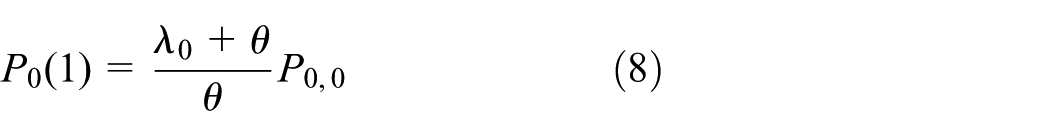
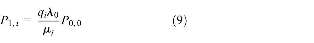
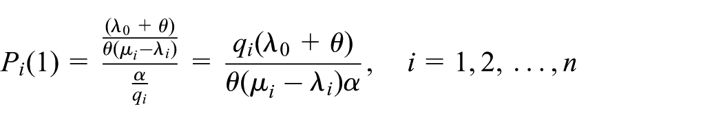
If the stability condition ${\rho }_i={\lambda }_i/{\mu }_i<1$ , $i=1,2,\dots ,n$ , holds, the PGF of the steady-state queue length is given by

$$\begin{array}{cc}\multicolumn{1}{c}{P(z)}& =P_0(z)+\sum _{i=1}^n{P}_i(z)\hfill \\ \multicolumn{1}{c}{}& =\frac{({\lambda }_0+\theta )}{{\lambda }_0(1-z)+\theta }\{1+{\lambda }_{0}z\sum _{i=1}^n\frac{q_i}{{\mu }_i-{\lambda }_{i}z}\}{P}_{0,0}\hfill \end{array}$$

(13)

where

$$P_{0,0}=\frac{1}{\alpha {\lambda }_0},\alpha =\frac{{\lambda }_0+\theta }{{\lambda }_0\theta }+\sum _{i=1}^n\frac{q_i({\lambda }_0+\theta )}{\theta ({\mu }_i-{\lambda }_i)}$$

(14)

Performance measure

In this section, we will determine some interesting performance measures of the system.

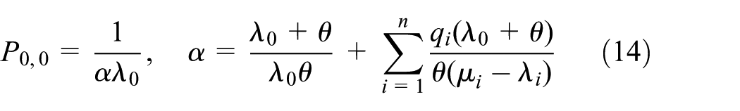
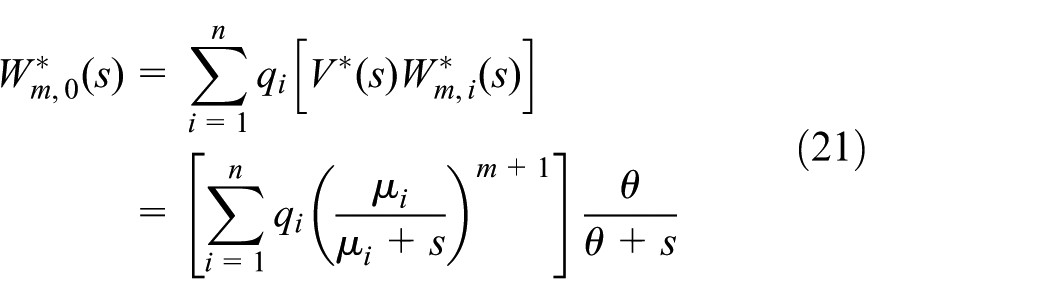
Let $L$ be the number of customers in the system. Then, taking derivative of $P(z)$ at $z=1$ , we have average number of customers in the system as follows

$$\begin{array}{cc}\multicolumn{1}{c}{E(L)}& =P\prime (1)=\frac{{\lambda }_0({\lambda }_0+\theta )}{{\theta }^2}{P}_{0,0}\hfill \\ \multicolumn{1}{c}{}& +\sum _{i=1}^n\frac{q_i{\lambda }_0({\lambda }_0+\theta )[{\lambda }_0({\mu }_i-{\lambda }_i)+{\mu }_i\theta ]}{{\theta }^2{({\mu }_i-{\lambda }_i)}^2}{P}_{0,0}\hfill \\ \multicolumn{1}{c}{}& =\frac{{\lambda }_0+\theta }{\alpha {\theta }^2}\{1+\sum _{i=1}^n\frac{q_i[{\lambda }_0({\mu }_i-{\lambda }_i)+{\mu }_i\theta ]}{{({\mu }_i-{\lambda }_i)}^2}\}\hfill \end{array}$$

(15)

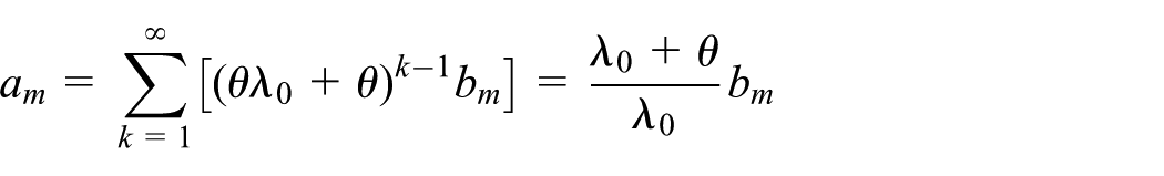
Next, we analyze the average time that the system resides in vacation phase $0$ . It is easy to know that the probability of no customer arrival during a vacation is $\theta /({\lambda }_0+\theta )$ , that is, the probability that there are customers in the system at the end of vacation is ${\lambda }_0/({\lambda }_0+\theta )$ . We know that if the system is empty when a vacation ends, another vacation begins, otherwise, the system jumps from the vacation phase to some operative phase $i$ . So, the number of vacation in phase $0$ is distributed with geometric distribution with parameter ${\lambda }_0/({\lambda }_0+\theta )$ . Therefore, the average number of vacation is $({\lambda }_0+\theta )/{\lambda }_0$ . Because the vacation time is exponentially distributed with rate $\theta$ , the average time of vacation is $1/\theta$ . Hence, the average time that the system resides in vacation phase $0$ is $({\lambda }_0+\theta )/{\lambda }_0\theta$ .

Using the above result, the average number of customers at the end of phase $0$ is ${\lambda }_0\times (({\lambda }_0+\theta )/{\lambda }_0\theta )=({\lambda }_0+\theta )/\theta$ , which is the product of the average time residing in phase $0$ and arrival rate of customer in phase $0$ . That is to say, the average number of customers at the beginning of some operative phase $i$ is $({\lambda }_0+\theta )/\theta$ . So, the average duration of time that the system resides in operative phase $i$ is $({\lambda }_0+\theta )/[\theta ({\mu }_i-{\lambda }_i)]$ , where $1/({\mu }_i-{\lambda }_i)$ is the mathematical expectation of busy period that one customer induces in phase $i$ .

From equations (5) and (12), the system is in phase $0$ with probability

$$P_0(1)=\frac{{\lambda }_0+\theta }{{\lambda }_0\theta \alpha }$$

(16)

Intuitively, the probability that the system is in phase $0$ is equal to the long-run proportion of time during which the system resides in phase $0$ . From the renewal-reward theorem, we have

$$P_0(1)=\frac{\frac{{\lambda }_0+\theta }{{\lambda }_0\theta }}{\frac{{\lambda }_0+\theta }{{\lambda }_0\theta }+\sum _{i=1}^n\frac{q_i({\lambda }_0+\theta )}{\theta ({\mu }_i-{\lambda }_i)}}=\frac{{\lambda }_0+\theta }{{\lambda }_0\theta \alpha }$$

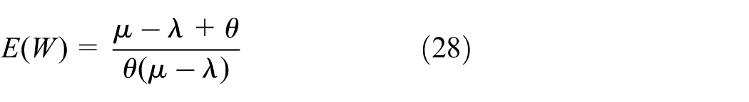
where $\alpha$ represents the average time between two consecutive instants at which a vacation phase commences, that is, the average length of a cycle, and $\sum _{i=1}^n(q_i({\lambda }_0+\theta )/\theta ({\mu }_i-{\lambda }_i))$ is the average length of working time in this cycle. The detailed calculation of the average length of working time in this cycle will be presented below (see equation (27)).

Similarly, the probability that the system is in phase $i$ , $i=1,2,\dots ,n$ , is equal to

$$\begin{array}{c}\hfill P_i(1)=\frac{\frac{q_i({\lambda }_0+\theta )}{\theta ({\mu }_i-{\lambda }_i)}}{\frac{{\lambda }_0+\theta }{{\lambda }_0\theta }+\sum _{i=1}^n\frac{q_i({\lambda }_0+\theta )}{\theta ({\mu }_i-{\lambda }_i)}}=\frac{q_i({\lambda }_0+\theta )}{\theta ({\mu }_i-{\lambda }_i)\alpha }\hfill \end{array}$$

(17)

which can also be derived by equation (10).

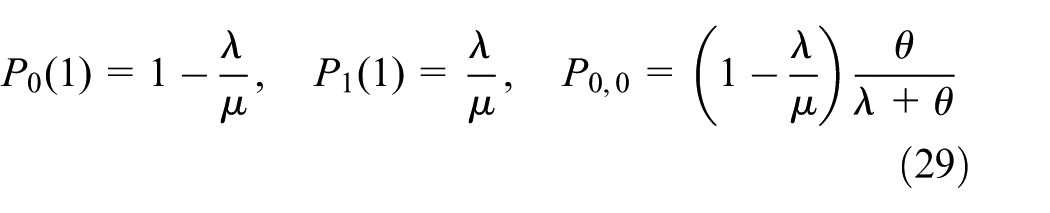
Moreover, the probability that the system is empty is

$$P_{0,0}=\frac{1}{\alpha {\lambda }_0}$$

(18)

It can also be explained by renewal-reward theorem. The average time required for one customer arrival in phase $0$ is $1/{\lambda }_0$ . So, the proportion of time the system resides in state $(0,0)$ is given by

$$P_{0,0}=\frac{(1/{\lambda }_0)}{\alpha }=\frac{1}{\alpha {\lambda }_0}$$

Now, cycle analysis will be given. A cycle is defined as the duration of time between two consecutive instants of phase $i$ beginning, $i=0,1,2,\dots ,n$ . Then, we have $(n+1)$ types of cycles. Let $C_i$ be the length of type $i$ cycle, $i=0,1,2,\dots ,n$ . Obviously, $E(C_0)=\alpha$ . Next, we analyze $E(C_i)$ , $i=1,2,\dots ,n$ .

During type $i$ cycle, the probability that the system visits the phase $0$ $k$ times is $(1-q_i{)}^{k-1}{q}_i$ , where $k=1,2,\dots$ , and the average length of the cycle in this case is

$$\begin{array}{l}\frac{{\lambda }_0+\theta }{\theta ({\mu }_i-{\lambda }_i)}+\frac{{\lambda }_0+\theta }{{\lambda }_0\theta }+(k-1)\\ \left(\frac{{\lambda }_0+\theta }{{\lambda }_0\theta }+{\displaystyle \sum _{j=1,j\ne i}^n\frac{q_j({\lambda }_0+\theta )}{\theta ({\mu }_j-{\lambda }_j)(1-q_i)}}\right)\end{array}$$

Hence, we can obtain that

$$\begin{array}{cc}\multicolumn{1}{c}{E(C_i)}& =\sum _{k=1}^{\infty }{(1-q_i)}^{k-1}{q}_i[\frac{{\lambda }_0+\theta }{\theta ({\mu }_i-{\lambda }_i)}+\frac{{\lambda }_0+\theta }{{\lambda }_0\theta }+(k-1)(\frac{{\lambda }_0+\theta }{{\lambda }_0\theta }+\sum _{j=1,j\ne i}^n\frac{q_j({\lambda }_0+\theta )}{\theta ({\mu }_j-{\lambda }_j)(1-q_i)})]\hfill \\ \multicolumn{1}{c}{}& =\frac{{\lambda }_0+\theta }{\theta ({\mu }_i-{\lambda }_i)}+\frac{{\lambda }_0+\theta }{{\lambda }_0\theta }+\sum _{k=1}^{\infty }(k-1)(1-q_i{)}^{k-1}{q}_i[\frac{{\lambda }_0+\theta }{{\lambda }_0\theta }+(\alpha -\frac{{\lambda }_0+\theta }{{\lambda }_0\theta }-\frac{q_i({\lambda }_0+\theta )}{\theta ({\mu }_i-{\lambda }_i)})\frac{1}{(1-q_i)}]\hfill \\ \multicolumn{1}{c}{}& =\frac{{\lambda }_0+\theta }{\theta ({\mu }_i-{\lambda }_i)}+\frac{{\lambda }_0+\theta }{{\lambda }_0\theta }+\frac{(1-q_i)}{q_i}[\frac{{\lambda }_0+\theta }{{\lambda }_0\theta }+(\alpha -\frac{{\lambda }_0+\theta }{{\lambda }_0\theta }-\frac{q_i({\lambda }_0+\theta )}{\theta ({\mu }_i-{\lambda }_i)})\frac{1}{(1-q_i)}]\hfill \\ \multicolumn{1}{c}{}& =\frac{{\lambda }_0+\theta }{\theta ({\mu }_i-{\lambda }_i)}+\frac{{\lambda }_0+\theta }{{\lambda }_0\theta }+\frac{(1-q_i)}{q_i}[\frac{{\lambda }_0+\theta }{{\lambda }_0\theta }-\frac{q_i}{(1-q_i)}+(\alpha -\frac{q_i({\lambda }_0+\theta )}{\theta ({\mu }_i-{\lambda }_i)})\frac{1}{(1-q_i)}]\hfill \\ \multicolumn{1}{c}{}& =\frac{{\lambda }_0+\theta }{\theta ({\mu }_i-{\lambda }_i)}+\frac{1}{q_i}(\alpha -\frac{q_i({\lambda }_0+\theta )}{\theta ({\mu }_i-{\lambda }_i)})=\alpha q_i\hfill \end{array}$$

(19)

for $i=1,2,\dots ,n$ . By equation (19) and renewal-reward theorem, we can also obtain the probability that the system resides in phase $i$

$$P_i(1)=\frac{\frac{({\lambda }_0+\theta )}{\theta ({\mu }_i-{\lambda }_i)}}{\frac{\alpha }{q_i}}=\frac{q_i({\lambda }_0+\theta )}{\theta ({\mu }_i-{\lambda }_i)\alpha },i=1,2,\dots ,n$$

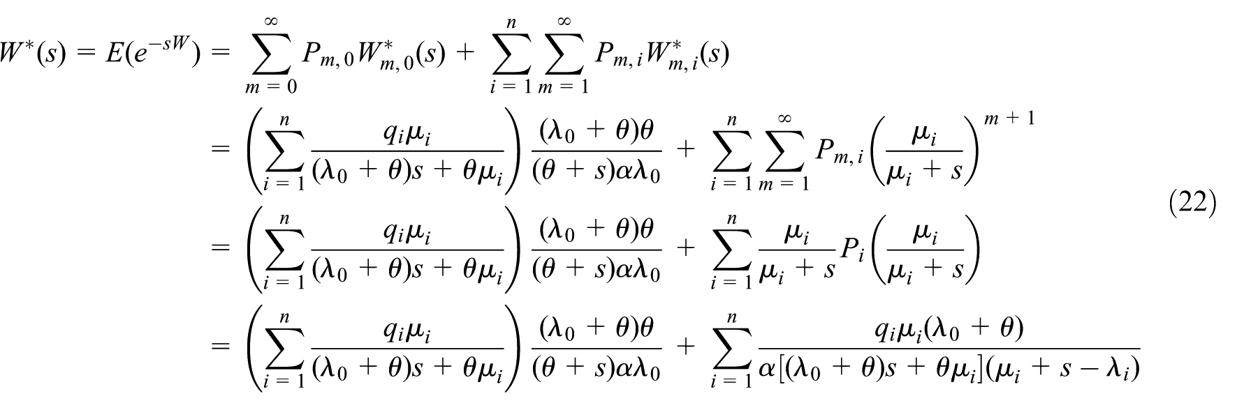
The sojourn time of a customer is an important performance measure. We will derive the Laplace–Stieltjes transform (LST) of the stationary sojourn time distribution of an arbitrary customer. Let $W$ and $W_{m,i}$ be the stationary sojourn time of an arbitrary customer and a customer that arrives to the system when it is in state $(m,i)$ , respectively.

When a customer arrives in state $(m,i)$ , $m=1,2,\cdots ,$ $i=1,2,\dots ,n$ , the sojourn time until departure is the sum of $(m+1)$ service completions, which has Erlang distribution with $(m+1)$ stages and parameter ${\mu }_i$ . That is, $W_{m,i}~\mathrm{Erlang}({\mu }_i,m+1)$ . And its LST is

$$W_{m,i}^{*}(s)=E(e^{-s{W}_{m,i}})={\left(\frac{{\mu }_i}{{\mu }_i+s}\right)}^{m+1}$$

(20)

where ${\mu }_i/({\mu }_i+s)$ is the LST of service time distribution in phase $i$ .

When a customer arrives in state $(m,0)$ , $m=0,1,2,\dots$ , the sojourn time until departure is the sum of residual vacation time and the service times of $(m+1)$ customers. Note that the residual vacation time is identically distributed with vacation time, and the system moves from phase $0$ to phase $i$ with probability $q_i$ , $i=1,2,\dots ,n$ , where $q_i>0$ , $\sum _{i=1}^n{q}_i=1$ . Combining all these things, we have

$$\begin{array}{l}{W}_{m,0}^{\ast }(s)={\displaystyle \sum _{i=1}^n{q}_i}\left[V^{\ast }(s)W_{m,i}^{\ast }(s)\right]\\ =\left[{\displaystyle \sum _{i=1}^n{q}_i}{\left(\frac{{\mu }_i}{{\mu }_i+s}\right)}^{m+1}\right]\frac{\theta }{\theta +s}\end{array}$$

(21)

where $W_{m,0}^{*}(s)$ and $V^{*}(s)$ are the LST of sojourn time $W_{m,0}$ and vacation time $V$ , respectively.

Then, the LST of the stationary sojourn time distribution of an arbitrary customer can be given as follows

$$\begin{array}{cc}\multicolumn{1}{c}{W^{*}(s)=E(e^{-\mathrm{sW}})}& =\sum _{m=0}^{\infty }{P}_{m,0}{W}_{m,0}^{*}(s)+\sum _{i=1}^n\sum _{m=1}^{\infty }{P}_{m,i}{W}_{m,i}^{*}(s)\hfill \\ \multicolumn{1}{c}{}& =\left(\sum _{i=1}^n\frac{q_i{\mu }_i}{({\lambda }_0+\theta )s+\theta {\mu }_i}\right)\frac{({\lambda }_0+\theta )\theta }{(\theta +s)\alpha {\lambda }_0}+\sum _{i=1}^n\sum _{m=1}^{\infty }{P}_{m,i}{\left(\frac{{\mu }_i}{{\mu }_i+s}\right)}^{m+1}\hfill \\ \multicolumn{1}{c}{}& =\left(\sum _{i=1}^n\frac{q_i{\mu }_i}{({\lambda }_0+\theta )s+\theta {\mu }_i}\right)\frac{({\lambda }_0+\theta )\theta }{(\theta +s)\alpha {\lambda }_0}+\sum _{i=1}^n\frac{{\mu }_i}{{\mu }_i+s}{P}_i\left(\frac{{\mu }_i}{{\mu }_i+s}\right)\hfill \\ \multicolumn{1}{c}{}& =\left(\sum _{i=1}^n\frac{q_i{\mu }_i}{({\lambda }_0+\theta )s+\theta {\mu }_i}\right)\frac{({\lambda }_0+\theta )\theta }{(\theta +s)\alpha {\lambda }_0}+\sum _{i=1}^n\frac{q_i{\mu }_i({\lambda }_0+\theta )}{\alpha [({\lambda }_0+\theta )s+\theta {\mu }_i]({\mu }_i+s-{\lambda }_i)}\hfill \end{array}$$

(22)

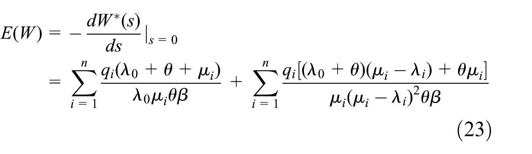
Using equation (22), the average sojourn time of an arbitrary customer is derived by

$$\begin{array}{cc}\multicolumn{1}{c}{E(W)}& =-\frac{d{W}^{*}(s)}{\mathrm{ds}}{|}_{s=0}\hfill \\ \multicolumn{1}{c}{}& =\sum _{i=1}^n\frac{q_i({\lambda }_0+\theta +{\mu }_i)}{{\lambda }_0{\mu }_i\theta \beta }+\sum _{i=1}^n\frac{q_i[({\lambda }_0+\theta )({\mu }_i-{\lambda }_i)+\theta {\mu }_i]}{{\mu }_i{({\mu }_i-{\lambda }_i)}^2\theta \beta }\hfill \end{array}$$

(23)

where

$$\beta =\frac{1}{{\lambda }_0}+\sum _{i=1}^n\frac{q_i}{{\mu }_i-{\lambda }_i}$$

Finally, we give the LST of the length of working time in the type $0$ cycle. That is, we give the LST of the length of working time in the time interval between two consecutive instants of phase $0$ commencing.

Assume that the system is in state $(m,i)$ when the working time begins, where $m=1,2,\dots$ , $i=1,2,\dots ,n$ . And in this case, we define $U_{m,i}$ and $U_{m,i}^{*}(s)$ as the length of working time and its LST, respectively. Then, $U_{m,i}$ and $U_{m,i}^{*}(s)$ are also the length of busy period caused by $m$ customers and its LST, respectively. Obviously, we have

$$U_{m,i}^{*}(s)={[U_{1,i}^{*}(s)]}^m$$

where $U_{1,i}^{*}(s)$ is determined by $U_{1,i}^{*}(s)=B_i^{*}(s+{\lambda }_i-{\lambda }_i{U}_{1,i}^{*}(s))$ , and $B_i^{*}(s)={\mu }_i/({\mu }_i+s)$ is the LST of service time distribution.

We denote by $U$ and $U^{*}(s)$ the length of working time in the type $0$ cycle and its LST, respectively. Let $a_m$ be the probability that there are $m$ arrivals during phase $0$ , and $b_m$ be the probability that $m$ customers arrive during a vacation. Then, we can easily get

$$b_m=\underset{0}{\overset{\infty }{\int }}\theta \frac{{({\lambda }_{0}t)}^m}{m!}{e}^{-({\lambda }_0+\theta )t}\mathrm{dt}$$

and

$$a_m=\sum _{k=1}^{\infty }\left[{(\theta {\lambda }_0+\theta )}^{k-1}{b}_m\right]=\frac{{\lambda }_0+\theta }{{\lambda }_0}{b}_m$$

where $\theta /({\lambda }_0+\theta )$ is the probability that there are no arrivals during a vacation.

Combining all the things, we have

$$\begin{array}{cc}\multicolumn{1}{c}{U^{*}(s)}& =\sum _{i=1}^n{q}_i[\sum _{m=1}^{\infty }{a}_m{U}_{m,i}^{*}(s)]=\sum _{i=1}^n{q}_i\left\{\sum _{m=1}^{\infty }{a}_m{[U_{1,i}^{*}(s)]}^m\right\}\hfill \\ \multicolumn{1}{c}{}& =\frac{({\lambda }_0+\theta )}{{\lambda }_0}\sum _{i=1}^n{q}_i\left\{\sum _{m=1}^{\infty }{b}_m{[U_{1,i}^{*}(s)]}^m\right\}\hfill \end{array}$$

(24)

Thus, the average length of working time in the type $0$ cycle is

$$\begin{array}{cc}\multicolumn{1}{c}{E(U)}& =-\frac{d{U}^{*}(s)}{\mathrm{ds}}{|}_{s=0}=-\frac{({\lambda }_0+\theta )}{{\lambda }_0}\hfill \\ \multicolumn{1}{c}{}& \sum _{i=1}^n{q}_i\left\{\sum _{m=1}^{\infty }{b}_{m}m{[U_{1,i}^{*}(s)]}^{m-1}\frac{{\mathrm{dU}}_{1,i}^{*}(s)}{\mathrm{ds}}\right\}{|}_{s=0}\hfill \\ \multicolumn{1}{c}{}& =\frac{({\lambda }_0+\theta )}{{\lambda }_0}\sum _{i=1}^n{q}_i\left(\sum _{m=1}^{\infty }{b}_m\frac{m}{{\mu }_i-{\lambda }_i}\right)\hfill \\ \multicolumn{1}{c}{}& =\frac{({\lambda }_0+\theta )\theta }{{\lambda }_0}\sum _{i=1}^n{q}_i\frac{1}{{\mu }_i-{\lambda }_i}\underset{0}{\overset{\infty }{\int }}\sum _{m=1}^{\infty }\frac{{({\lambda }_{0}t)}^m}{(m-1)!}{e}^{-({\lambda }_0+\theta )t}\mathrm{dt}\hfill \\ \multicolumn{1}{c}{}& =\frac{({\lambda }_0+\theta )\theta }{{\lambda }_0}\sum _{i=1}^n{q}_i\frac{1}{{\mu }_i-{\lambda }_i}\frac{{\lambda }_0}{{\theta }^2}\hfill \\ \multicolumn{1}{c}{}& =\sum _{i=1}^n\frac{q_i({\lambda }_0+\theta )}{\theta ({\mu }_i-{\lambda }_i)}\hfill \end{array}$$

(25)

Special case

A special case of our model introduced in section “Model description” is when $n=1$ . That is, there are only one operative phase and one vacation phase. Assuming that the arrival rates are homogeneous, that is, ${\lambda }_0={\lambda }_i=\lambda$ . Then, our model translates into a classical $M/M/1$ queues with multiple vacations. Let ${\mu }_i=\mu$ . From equations (13) and (14), the PGF of the steady-state queue length is

$$P(z)=\left(\frac{1-\lambda /\mu }{1-(\lambda /\mu )z}\right)\left(\frac{\theta }{\lambda (1-z)+\theta }\right)$$

(26)

The average steady-state queue length is

$$E(L)=\frac{\lambda (\mu -\lambda +\theta )}{\theta (\mu -\lambda )}$$

(27)

The average sojourn time of an arbitrary customer is

$$E(W)=\frac{\mu -\lambda +\theta }{\theta (\mu -\lambda )}$$

(28)

From equations (27) and (28), the Littles law formula, $E(W)=E(L)/\lambda$ , follows

We can also get

$$P_0(1)=1-\frac{\lambda }{\mu },P_1(1)=\frac{\lambda }{\mu },P_{0,0}=(1-\frac{\lambda }{\mu })\frac{\theta }{\lambda +\theta }$$

(29)

Another special case of our model introduced in section “Model description” is when the system is homogeneous, that is, all arrival rates and service rates are equal. In this case, our model also translates into $M/M/1$ queues with multiple vacations. Substituting ${\lambda }_0={\lambda }_1=\cdots ={\lambda }_n$ and ${\mu }_1={\mu }_2=\cdots ={\mu }_n$ into equation (13), we obtain the PGF of the steady-state queue length as follows

$$P(z)=\left(\frac{1-\lambda /\mu }{1-(\lambda /\mu )z}\right)\left(\frac{\theta }{\lambda (1-z)+\theta }\right)$$

(30)

Note that equations (26) and (30) are the same.

Servi and Finn ² discussed $M/M/1$ queues with multiple working vacation. Assume in Servi and Finn ² that service rate ${\mu }_V=0$ during the working vacation. The model in this case coincides with our two special models. Of course, the aforementioned results are the same as well. Also, if we assume the service time distribution is exponential with parameter $\mu$ in Tian and Zhang’s system (Tian and Zhang, ⁸ Theorem $2.2.1$ , p.19), equations (26) and (30) can be verified to be in agreement with the result of Theorem $2.2.1$ in Tian and Zhang. ⁸

Numerical results

In this section, based on the results obtained, we present some numerical examples to study the impact of the parameters on the average queue length and average sojourn time. Without loss of generality, we assume that $n=2$ , then the system has two operative phases and a vacation phase.

First, we assume that the system parameters are ${\lambda }_0=1,{\lambda }_1=1.2,{\lambda }_2=1.4,{\mu }_1=2,{\mu }_2=2.5$ . In Figure 2, we demonstrate the impact of the probability $q_1$ on the average queue length $E(L)$ for different vacation rate $\theta$ . Figure 2 indicates that $E(L)$ increases as $q_1$ increases when $\theta$ is equal to $0.5,1.0,\mathrm{and}1.5$ , respectively. On the other hand, if $q_1$ is fixed, $E(L)$ decreases as $\theta$ increases.

Figure 2.

The expected number of customers in the system $E(L)$ versus $q_1$ .

Second, in Figure 3, we demonstrate the impact of the service rate ${\mu }_2$ on the average queue length $E(L)$ for different values of $\theta$ . Assume that ${\lambda }_0=1,{\lambda }_1=1.2,{\lambda }_2=1.4,q_1=0.4,q_2=0.6$ . Figure 3 indicates that $E(L)$ decreases as ${\mu }_2$ increases when $\theta$ is equal to $0.5,1.0,\mathrm{and}1.5$ , respectively. On the other hand, if ${\mu }_2$ is fixed, $E(L)$ decreases as $\theta$ increases.

Figure 3.

The expected number of customers in the system $E(L)$ versus ${\mu }_2$ .

Third, in Figure 4, we demonstrate the impact of the probability $q_1$ on the average sojourn time $E(W)$ for different values of $\theta$ . Assume that the system parameters are ${\lambda }_0=1,{\lambda }_1=1.2,{\lambda }_2=1.4,{\mu }_1=2,{\mu }_2=2.5$ . Figure 4 indicates that $E(W)$ increases as $q_1$ increases when $\theta$ is equal to $0.5,1.0,\mathrm{and}1.5$ , respectively. On the other hand, if $q_1$ is fixed, $E(W)$ decreases as $\theta$ increases.

Figure 4.

The expected sojourn time $E(W)$ versus $q_1$ .

Next, in Figure 5, we demonstrate the impact of the service rate ${\mu }_2$ on the average sojourn time $E(W)$ for different values of $\theta$ . Assume that ${\lambda }_0=1,{\lambda }_1=1.2,{\lambda }_2=1.4,q_1=0.4,q_2=0.6$ . Figure 5 indicates that $E(W)$ decreases as ${\mu }_2$ increases for all different $\theta$ . On the other hand, if ${\mu }_2$ is fixed, $E(W)$ decreases as $\theta$ increases.

Figure 5.

The expected sojourn time $E(W)$ versus ${\mu }_2$ .

Finally, suppose that ${\lambda }_0=1,{\lambda }_1=1.2,{\lambda }_2=1.4,{\mu }_1=2,\theta =1.5$ . We present some numerical results of $E(L)$ for ${\mu }_2=1.5,1.6,\dots ,2.4$ and $q_1=0.10,0.25,\dots ,1.0$ in Table 1. From Table 1, it is observed that for a fixed $q_1$ , $E(L)$ decreases as ${\mu }_2$ increases. Also, it is observed that for ${\mu }_2\le 2.2$ , $E(L)$ decreases as $q_1$ increases; however, for ${\mu }_2\ge 2.3$ , $E(L)$ increases as $q_1$ increases. Note that the critical value of ${\mu }_2$ is not equal to ${\mu }_1$ , that is, 2. This is true because of the effect of random environment.

Table 1.

The expected number of customers in the system $E(L)$ versus $q_1$ and ${\mu }_2$ .

${\mu }_2$	q 1
	0.10	0.25	0.40	0.55	0.70	0.85	1.0
	E(L)
1.5	14.0309	13.5213	12.8333	11.8535	10.3462	7.7281	2.0556
1.6	7.1222	6.7469	6.2778	5.6746	4.8704	3.7444	2.0556
1.7	4.8636	4.5874	4.2619	3.8725	3.3986	2.8089	2.0556
1.8	3.7593	3.5588	3.3333	3.0778	2.7857	2.4487	2.0556
1.9	3.1120	2.9711	2.8185	2.6527	2.4717	2.2735	2.0556
2.0	2.6905	2.5976	2.5000	2.3974	2.2895	2.1757	2.0556
2.1	2.3963	2.3427	2.2879	2.2318	2.1744	2.1157	2.0556
2.2	2.1806	2.1597	2.1389	2.1181	2.0972	2.0764	2.0556
2.3	2.0163	2.0232	2.0299	2.0365	2.0430	2.0493	2.0556
2.4	1.8877	1.9198	1.9476	1.9760	2.0034	2.0299	2.0556

Conclusion

In this article, we studied an $M/M/1$ queue with vacation in a multi-phase random environment. For this model, we obtained the PGF of the steady-state queue length at arbitrary epoch. Performance measures such as the average queue length, the average length of a cycle, and the probability that the system is in phase $i$ were also presented. Furthermore, we obtained the LST of the steady-state sojourn time distribution of an arbitrary customer and the server’s working time distribution in a cycle, respectively. We investigated two special cases of our model. Finally, we gave some numerical examples to demonstrate the impact of parameters on the average queue length and the average sojourn time, respectively.