Gibbs-like phenomenon inherent in a lumped element model of a rod

Abstract

The underlying assumption of a lumped element model is that a spatially distributed physical system can be approximated by a topology of discrete entities. The impact of this assumption is illustrated by a model of a finitely long elastic rod with uniform cross section. The model involves a cascade of masses and springs, where the boundary itself is driven by a step function. Previous authors have found closed-form solutions to related problems using the Laplace transform, while in this article we obtain closed-form solutions by eigenvalue decomposition. This means that the extension to a rod with non-uniform cross section is further illuminated. The closed-form solution is compared to a closed-form solution of a distributed parameter model. Both solutions involve a sum of a forward and a backward moving wave that travels with the speed of sound. In the case of the distributed parameter model, these waves are perfect square waves, while in the case of the lumped element model, these waves are imperfect square waves that are subjected to “Gibbs-like” ringing. Properties of this phenomenon are described. It is also shown that this phenomenon disappears, when using a continuous step function and a model with sufficiently many elements.

Introduction

Axial vibrations in a uniform rod is a canonical example that is described in a variety of mechanical and mathematical textbooks. Depending on the application, both distributed parameter models and mass-spring models are popular.

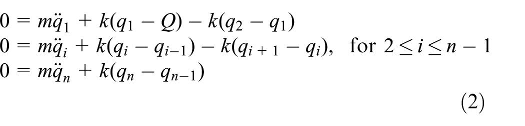
Distributed parameter models involve solving a partial differential equation with boundary and initial conditions. In Benaroya, ¹ a closed-form solution for a distributed parameter model is given for a rod that is fixed on one side and free to move on the other side. This is the physical problem that is discussed in this article. The only extension is that the rod is initially disturbed by a step input.

A mass-spring model is a type of lumped element model that involves solving a system of ordinary differential equations. It is commonly used in describing vibrations in mechanical systems. ² The simple mathematical description allows substantial interpretation and application of control theory, as discussed in Benaroya. ¹ Moreover, the mathematical descriptions are the same for a variety of analogous systems as well. This means that if progress is made on solving one problem, the actual impact is carried over to all other analogous systems. Some examples of analogous systems are described in Chapter 12 in Siddiqui and Singh. ³ In particular, it is shown that a system involving beam torsion and an electrical system is analogous to the problem described in this article.

Several papers exist on modeling an elastic horizontal rod as a cascade of masses and springs. An important contribution is Bavinck et al., ⁴ where closed-form solutions exist in the case when the velocity of the first left mass is subjected to a pulse response. The solution involves first finding the solution for a semi-infinite rod, which is a rod that has a starting point, but goes on forever. This becomes a linear system of second-order ordinary differential equations. The solution involves taking the Laplace transform to get rid of the derivatives. After resolving recurrence relations, the inverse Laplace transformation results in expressions that involve Bessel functions. Modeling a finite rod is done by superposing the solutions of two semi-infinite rods that are oppositely directed. Equations for free and fixed boundaries are dependent on whether the solutions are added or subtracted. The article also shows that the solutions are dependent on whether the mass or the spring comes first at the boundaries.

The model in this article is similar to the model in Bavinck et al., ⁴ when the rod is finitely long, starting with a spring on the left side that is fixed to a wall and ending with a mass on right side that is free to move. The differences between Bavinck et al. ⁴ and this article are related to the boundary on the left side. In this article, the left boundary itself is driven by a step function, while in Bavinck et al., ⁴ the left boundary is completely fixed and the velocity of the first mass is given a pulse load. It is possible that we could use the solution strategy of Bavinck et al., ⁴ to solve the problem in this article, but it is clearly not straightforward as such a derivation involves different recurrence relations that need to be solved and converted into Chebyshev polynomials before the inverse Laplace transform can be done.

Another closely related paper is Dieterman et al., ⁵ which compares a distributed parameter model of a semi-infinite rod with the models described in Bavinck et al. ⁴ The main focus is on harmonic and transient behavior, but also the topic of step response is touched on. It is shown that a Gibbs-like pattern appears and this complies with the results in this article.

The last paper that is close to the current contribution is Bavinck and Dieterman, ⁶ which contains a model for the movement of a train, where the locomotive is able to have different mass than the wagons. The papers Bavinck et al., ⁴ Dieterman et al., ⁵ and Bavinck and Dieterman ⁶ are linked together as they use the Laplace transform to find the solutions. This has the advantage of mathematical simplicity, when the masses and the springs are essentially the same, except on the boundaries. However, it seems difficult to generalize these ways to yield any configuration of stiffnesses and masses.

In this article, we have therefore chosen a different route to solving the problem which involves eigenvalue decomposition. We have found closed-form solutions when the masses and springs are equal, but the solutions are easily expandable by numerical eigenvalue decompositions.

The mathematical description leads to a system of linear ordinary differential equations that is given on a matrix form. These equations are coupled, but they can be decoupled by an eigenvalue decomposition.

In Smith and Smith, ² a closed-form solution is found when the number of elements is limited to two, while the extension to $n$ elements is described in Demmel. ⁷ In Demmel, ⁷ various numerical algorithms for finding eigenvalues and eigenvectors are given. Finally, the solution is interpreted in terms of eigenmodes. An eigenmode is a natural vibration mode, where all parts move sinusoidally with the same frequency.

There are two artifacts of the mass-spring model compared to the distributed parameter model. One artifact is related to the numerical algorithm of finding the eigenvalue decomposition, which is described in Demmel. ⁷ The other artifact is related to the approximation that the mass of the beam is distributed on a finite number of distinct points along the rod.

This article differs from the approach in Demmel, ⁷ as it applies the closed-form expressions for the eigenvalues and eigenvectors that was found in Yueh. ⁸ This allows the solution to be fully closed-form. We show algebraically that the solution is a sum of a forward and a backward moving waves. This is analogous to the solution of the one-dimensional (1D) wave equation. Moreover, this extension allows us to prove that the “masses distributed on distinct points” approximation is dominating the numerical error in most applications. This artifact has much in common with the Gibbs phenomenon, which is described next.

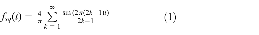
Using a Fourier expansion, we can represent a square wave with amplitude and cycle frequency equal to one by

$$\begin{array}{c}{f}_{\mathrm{sq}}(t)=\frac{4}{\pi }\sum _{k=1}^{\infty }\frac{\sin (2\pi (2k-1)t)}{2k-1}\hfill \end{array}$$

(1)

Therefore, $f_{\mathrm{sq}}(t)$ is a weighed sum of odd-integer harmonic frequencies. Computing any partial sum of this expansion leads to an imperfect square wave that contains a ringing artifact that is known as the Gibbs phenomenon.

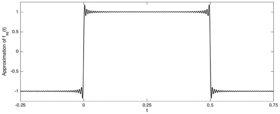
In Hewitt and Hewitt, ⁹ the Gibbs phenomenon is discussed in detail, but we give brief summary here. In Figure 1, the partial sum of the first $n=60$ terms is shown. It is well known that as $n$ goes to infinity, the frequency of the ringing increases, while the energy of the ringing goes to zero and the approximation approaches the square wave for any $t$ . It is peculiar that the level of overshoot and undershoot converges to a fixed value, which is $({\int }_0^1\mathrm{sinc}(x)\mathrm{dx}-1/2)a=0.089490a$ , where $a$ is twice the amplitude. Mathematically, this makes sense, since the point of overshooting and undershooting moves as a function of $n$ .

Figure 1.

The Gibbs phenomenon. The square wave is approximated by the partial sum of the first 60 terms in equation (1).

This article is laid out as follows: The first section contains both a distributed parameter model and a lumped element model of an elastic rod that is subjected to a step input source. In the second section, the imperfect square wave that is obtained in the lumped element model is discussed in more detail. In the third section, the impact of using a continuous step function is outlined. It is suggested that for any steepness, it is possible to choose enough elements to remove the ringing.

Sequential mass-spring model of a rod

We consider a horizontal rod of relaxed length $L$ , mass $M$ , and stiffness $K$ that is sliding frictionless on a table. We model the rod as a set of $n$ blocks that are connected by $n$ spring elements (Figure 2). All blocks have mass $m=M/n$ and all springs have relaxed length $h$ and spring constant $k=\mathrm{Kn}$ . The blocks have zero length, so $h=L/n$ . The springs are free to rotate with respect to the blocks, which means that the springs cannot take up angular momentum. A 1D coordinate system is introduced, where positive x-axis is to the right. The left side of the rod has the coordinate $Q$ and this is also the position of left side of the first spring. The origin of the coordinate system is chosen so that $Q(0)=0$ .

Figure 2.

The model of the rod contains $n=9$ blocks and $n=9$ springs. The figure shows the initial position, where $Q(0)=0$ and all springs are neither tensioned nor compressed. The generalized coordinate $q_i$ is defined as the movement away from $\mathrm{ih}$ .

In the case when all springs are not in compression or in tension and $Q(0)=0$ , the center of block $i$ is $\mathrm{ih}$ . This is the situation that is illustrated in Figure 2. The distance between $\mathrm{ih}$ and $Q_i(t)$ is $q_i(t)$ , that is $Q_i(t)=\mathrm{ih}+q_i(t)$ . The physical state of the rod is therefore uniquely defined by $Q(t)$ and the generalized coordinates $q_i(t)\mathrm{s}$ . In other words, the state space of the system is n-dimensional.

Newton’s second law on each element is given by

$$\begin{array}{c}0=m{\stackrel{··}{q}}_1+k(q_1-Q)-k(q_2-q_1)\hfill \\ \multicolumn{1}{c}{0=m{\stackrel{··}{q}}_i+k(q_i-q_{i-1})-k(q_{i+1}-q_i),\mathrm{for}2\le i\le n-1}\\ \multicolumn{1}{c}{0=m{\stackrel{··}{q}}_n+k(q_n-q_{n-1})}\end{array}$$

(2)

There are two ways to proceed on solving this system: the distributed parameter model and the lumped element model.

The distributed parameter model

We write the middle equation in equation (2) as

$$\begin{array}{c}{\stackrel{··}{q}}_i=\frac{K{L}^2}{M}\frac{(q_{i-1}-2q_i+q_{i+1})}{h^2}\hfill \end{array}$$

and let $n$ go to infinity. This means that $h$ goes to zero and we obtain the 1D wave equation

$$\begin{array}{c}\frac{{\partial }^{2}q}{\partial t^2}=c^2\frac{{\partial }^{2}q}{\partial x^2}\hfill \end{array}$$

where $q(x,t)$ is the continuous function of movement and $c$ is the wave propagation speed. This is seen because $K=\mathrm{EA}/L$ , $M=\rho \mathrm{AL}$ , and $c=\sqrt{E/\rho }$ , where $E$ is Young’s modulus and $\rho$ is mass density of the rod.

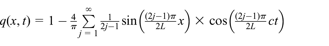
In this article, we study the behavior when we apply a unit step input at the left boundary and zero initial conditions. At the left boundary, we have $q(0,t)=1$ , while at the right boundary we have always zero momentum, that is, $\partial q(x,t)/\partial x=0$ . The initial conditions are $q(x,0)=0$ and $\partial q(x,t)/\partial t{|}_{t=0}=0$ . Note that this could also be modeled by setting $q(0,t)=0$ and applying a step function as a driving force. However, we chose this path since we can apply the derivation in on page 510 in Benaroya. ¹ In Benaroya, ¹ the equations are developed for $q(0,t)=0$ and arbitrary initial conditions. We solved this by calling $u(x,t)=q(x,t)-1$ , finding the solution and substituting back again

$$\begin{array}{l}\begin{array}{l}q(x,t)=1+{\displaystyle \sum _{j=1}^{\infty }}\sin \left(\frac{(2j-1)\pi }{2L}x\right)\hfill \\ \times \left(A_j\cos \left(\frac{(2j-1)\pi }{2L}ct\right)+B_j\sin \left(\frac{(2j-1)\pi }{2L}ct\right)\right)\hfill \end{array}\hfill \end{array}$$

Using $\partial q(x,t)/\partial t{|}_{t=0}=0$ , we see that all $B_j\mathrm{s}$ are zero. Moreover, $q(x,0)=0$ implies that $A_j$ must be equal to $-4/(\pi (2j-1))$ . Therefore

$$\begin{array}{c}q(x,t)=1-\frac{4}{\pi }\sum _{j=1}^{\infty }\frac{1}{2j-1}\sin \left(\frac{(2j-1)\pi }{2L}x\right)\times \cos \left(\frac{(2j-1)\pi }{2L}\mathrm{ct}\right)\hfill \end{array}$$

and using that $\sin (\alpha )\cos (\beta )=(\sin (\alpha +\beta )+\sin (\alpha -\beta ))/2$ , we obtain

$$\begin{array}{c}q(x,t)=\frac{f((x+\mathrm{ct})/4L)+f((x-\mathrm{ct})/4L)}{2},\mathrm{where}f(u)=1-f_{\mathrm{sq}}(u)\hfill \end{array}$$

(3)

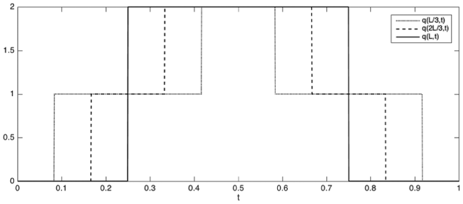
Clearly, $q(x,t)$ is a sum of two square waves with frequency $c/(4L)$ that moves in opposite directions. The sum of these square waves at three locations is described in Figure 3. The time period of these waves is independent of $x$ and equal to $4L/c$ . At the end point $x=L$ , the point moves to two after the sound wave has propagated down to this point. It stays there till the sound has propagated to the other end and back again. At this time, the point jumps back to zero again. The end point is just a square wave with phase shift equal to one-fourth of the wave period. By equation (3), we see that $q(L,t)=f((L+\mathrm{ct})/(4L))$ .

Figure 3.

$q(x,t)$ at three different locations in the rod.

At the point $x=L/3$ , the point moves to one after the wave has reached this point. It stays at this location, till the sound wave has gone to the right end point and back again. The point moves to two. The wave is now going in the opposite direction and the $x=L/3$ point is not moving before the wave has reached the left side and back again. At this point, the point moves to one again. This is why we get this stair-like behavior that is seen in Figure 3. A similar discussion can be given for the time behavior at $x=2L/3$ . It is worth noting that if we approximate the $f_{\mathrm{sq}}$ by a partial sum of the Fourier expansion, we would obtain the Gibbs phenomenon on all the “corners” in Figure 3.

The lumped element model

We take a step back and see that equation (2) is a system of $n$ coupled second-order ordinary differential equations. This can be written on matrix form by

$$\begin{array}{c}\mathbf{M}\stackrel{··}{\mathit{q}}+\mathbf{K}\mathit{q}=\mathit{f}(t)\hfill \end{array}$$

(4)

where $\mathbf{M}$ is equal to $m\mathbf{I}$ and $\mathbf{K}$ is a tridiagonal matrix of the form

$$\begin{array}{c}k\left[\begin{array}{ccccccc}2\hfill & -1\hfill & 0\hfill & \dots \hfill & 0\hfill & 0\hfill & 0\hfill \\ \multicolumn{1}{c}{-1}& 2\hfill & -1\hfill & \dots \hfill & 0\hfill & 0\hfill & 0\hfill \\ \multicolumn{1}{c}{0}& -1\hfill & 2\hfill & \dots \hfill & 0\hfill & 0\hfill & 0\hfill \\ \multicolumn{1}{c}{⋮}& ⋮\hfill & ⋮\hfill & \ddots \hfill & ⋮\hfill & ⋮\hfill & ⋮\hfill \\ \multicolumn{1}{c}{0}& 0\hfill & 0\hfill & \dots \hfill & 2\hfill & -1\hfill & 0\hfill \\ \multicolumn{1}{c}{0}& 0\hfill & 0\hfill & \dots \hfill & -1\hfill & 2\hfill & -1\hfill \\ \multicolumn{1}{c}{0}& 0\hfill & 0\hfill & \dots \hfill & 0\hfill & -1\hfill & 1\hfill \end{array}\right]\hfill \end{array}$$

The first element of $\mathit{f}(t)$ is equal to $\mathrm{kQ}(t)$ , while the others are zero. In this context, $f_1(t)$ is referred to as the driving force of the system, even though the actual force that is applied is $f_1(t)-k{q}_1$ .

If $\mathbf{K}$ was a diagonal matrix, then all equations would be decoupled and they could be solved separately. In fact, the equations would be harmonic oscillators, where properties are well known. Fortunately, there is a trick for decoupling equation (4), which is described in detail in Tisseur and Meerbergen. ¹⁰ Since both $\mathbf{M}$ and $\mathbf{K}$ are real symmetric and positive definite (i.e. ${\mathit{v}}^T\mathbf{M}\mathit{v}>0$ and ${\mathit{v}}^T\mathbf{K}\mathit{v}>0$ for any non-zero and real column vector $\mathit{v}$ ), then $(\mathbf{M},\mathbf{K})$ is a real definite pair.

When $(\mathbf{M},\mathbf{K})$ is a real definite pair, then solving the generalized eigenvalue problem

$$\begin{array}{c}\mathbf{M}\mathit{v}=\lambda \mathbf{K}\mathit{v}\hfill \end{array}$$

gives a diagonal matrix $\mathbf{D}$ of eigenvalues and a matrix of eigenvectors $\mathbf{V}$ . The important property that motivates this approach is that ${\mathbf{V}}^T\mathbf{MV}=\mathbf{I}$ and ${\mathbf{V}}^T\mathbf{KV}=\mathbf{D}$ , where $\mathbf{I}$ is the identity matrix.

If we now make another linear coordinate transformation $\mathbf{q}=\mathbf{V}\mathit{x}$ and also multiply equation (2) by ${\mathbf{V}}^T$ , we obtain

$$\begin{array}{c}\stackrel{··}{\mathit{x}}+\mathbf{D}\mathit{x}={\mathbf{V}}^T\mathit{f}(t)\hfill \end{array}$$

If we let ${\omega }_i=\sqrt{D_{\mathrm{ii}}}$ and the first element of the ith eigenvector is $V_{1i}$ , then

$$\begin{array}{c}{\stackrel{··}{x}}_i+{\omega }_i^2{x}_i=V_{1i}\mathrm{kQ}(t)\hfill \end{array}$$

(5)

These equations can be solved for any driving force using a superposition of a homogeneous solution and a particular solution. The homogeneous equation of equation (5) is equivalent to setting $Q(t)=0$ , which is

$$\begin{array}{cc}{x}_i(t)\hfill & =A_i\sin ({\omega }_{i}t+B_i)\hfill \end{array}$$

where the parameters $A_i$ and $B_i$ are determined from initial conditions. It is now clear that the natural frequency of the system is ${\omega }_i$ .

The usual way of finding particular solutions is by trying a more general form than $Q(t)$ which includes a number of constants and fitting it to equation (5). A more general way is to first change the second-order differential equation into a system of two first-order differential equations and then use integrating factors to find a more general term Adams. ¹¹ We rewrite equation (5) as

$$\begin{array}{l}{\stackrel{.}{y}}_i=A_i{y}_i+b_i(t),\mathrm{where}{y}_i=\left[\begin{array}{c}{x}_i(t)\hfill \\ {\stackrel{.}{x}}_i(t)\hfill \end{array}\right],\hfill \\ A_i=\left[\begin{array}{cc}0\hfill & 1\hfill \\ -{\omega }_i^2\hfill & 0\hfill \end{array}\right],\mathrm{and}{b}_i(t)=\left[\begin{array}{c}0\hfill \\ V_{1i}kQ(t)\hfill \end{array}\right]\hfill \end{array}$$

We seek a particular solution of the form ${\mathit{y}}_{i,p}=\exp (t{\mathbf{A}}_{\mathbf{i}}){\mathit{z}}_{\mathbf{i}}(t)$ . Consequently, we have that

$$\begin{array}{cc}\multicolumn{1}{c}{{\stackrel{·}{\mathit{y}}}_{\mathit{i},p}}& =\exp (t{\mathbf{A}}_{\mathbf{i}}){\mathbf{A}}_{\mathbf{i}}{\mathit{z}}_i(t)+\exp (t{\mathbf{A}}_{\mathbf{i}}){\stackrel{·}{\mathit{z}}}_i(t)\hfill \\ ={\mathbf{A}}_{\mathbf{i}}{\mathit{y}}_{\mathit{i},p}+\exp (t{\mathbf{A}}_{\mathbf{i}}){\stackrel{·}{z}}_{\mathit{i}}(t)\hfill \end{array}$$

where we are using the fact that $\exp (t{\mathbf{A}}_{\mathbf{i}}){\mathbf{A}}_{\mathbf{i}}={\mathbf{A}}_{\mathbf{i}}\exp (t{\mathbf{A}}_{\mathbf{i}})$ . This means that

$$\begin{array}{c}\exp (t{\mathbf{A}}_{\mathbf{i}}){\stackrel{·}{\mathit{z}}}_{\mathit{i}}(t)={\mathit{b}}_{\mathit{i}}(t)\mathrm{and}\hfill \\ {\mathit{z}}_i(t)=\underset{0}{\overset{t}{\int }}\exp (-u{\mathbf{A}}_{\mathbf{i}}){\mathit{b}}_{\mathit{i}}(u)\mathrm{du}+{\mathit{c}}_{\mathit{i}}\hfill \end{array}$$

and the particular solution is therefore

$$\begin{array}{c}{\mathit{y}}_{\mathit{i},p}=\underset{0}{\overset{t}{\int }}\exp ((t-u){\mathbf{A}}_{\mathbf{i}}){\mathit{b}}_{\mathit{i}}(u)\mathrm{du}+\exp (t{\mathbf{A}}_{\mathbf{i}}){\mathit{c}}_{\mathit{i}}\hfill \end{array}$$

(6)

where ${\mathit{c}}_{\mathit{i}}$ is found from the initial conditions of the problem. The exponential matrix $\exp (t{\mathbf{A}}_{\mathbf{i}})$ is of the form

$$\begin{array}{c}\exp (t{\mathbf{A}}_{\mathbf{i}})=s_{i,0}(t)\mathbf{I}+s_{i,1}{\mathbf{A}}_{\mathbf{i}}\mathrm{where}\hfill \\ s_{i,0}(t)=\frac{\alpha \exp (\beta t)-\beta \exp (\alpha t)}{\alpha -\beta }=\cos ({\omega }_{i}t)\hfill \\ s_{i,1}(t)=\frac{\exp (\alpha t)-\exp (\beta t)}{\alpha -\beta }=\frac{\sin ({\omega }_{i}t)}{{\omega }_i}\hfill \end{array}$$

by the Cayley–Hamilton theorem Gantmacher. ¹² Here, $\alpha =i{\omega }_i$ and $\beta =-i{\omega }_i$ are the roots of the characteristic polynomial of ${\mathbf{A}}_{\mathbf{i}}$ . Hence

$$\begin{array}{c}\exp (t{\mathbf{A}}_{\mathbf{i}})=\left[\begin{array}{cc}\cos ({\omega }_{i}t)\hfill & \frac{\sin ({\omega }_{i}t)}{{\omega }_i}\hfill \\ \multicolumn{1}{c}{-{\omega }_i\sin ({\omega }_{i}t)}& \cos ({\omega }_{i}t)\hfill \end{array}\right]\hfill \end{array}$$

and because we only need to look at the first element of ${\mathbf{y}}_{\mathbf{i}\mathbf{,}\mathbf{p}}$ in equation (6), then

$$\begin{array}{c}{x}_{i,p}(t)=\frac{V_{1i}k}{{\omega }_i}{\displaystyle \underset{0}{\overset{t}{\int }}\sin ({\omega }_i(t-u))Q(u)du+c_{i,1}\cos ({\omega }_{i}t)+c_{i,2}\sin ({\omega }_{i}t)}\hfill \end{array}$$

(7)

where $c_{i,1}$ and $c_{i,2}$ are the components of ${\mathit{c}}_i$ . We realize that the last two terms have the same form as the homogeneous solution. This means that if we redefine $A_i$ and $B_i$ , the full solution is

$$\begin{array}{c}{x}_i(t)=\frac{V_{1i}k}{{\omega }_i}\underset{0}{\overset{t}{\int }}\sin ({\omega }_i(t-u))Q(u)\mathrm{du}+A_i\sin ({\omega }_{i}t+B_i)\hfill \\ \multicolumn{1}{c}{\mathrm{and}{q}_j(t)=Q(t{)*}_t{S}_j(t)+\sum _{i=1}^n{V}_{\mathrm{ji}}{A}_i\sin ({\omega }_{i}t+B_i)}\\ \multicolumn{1}{c}{\mathrm{where}{S}_j(t)=k\sum _{i=1}^n[\frac{V_{\mathrm{ji}}{V}_{1i}}{{\omega }_i}\sin ({\omega }_{i}t)]}\end{array}$$

(8)

and ${*}_t$ is the convolution sign with respect to time.

Analytical expressions for $\mathbf{V}$ and $\mathbf{D}$

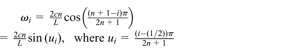
The normal approach for finding the $\mathbf{V}$ and $\mathbf{D}$ is to compute them numerically. However, in Theorem 1 in Yueh, ⁸ the eigenvalues and the eigenvectors are found analytically. That is

$$\begin{array}{c}{\omega }_i^2=\frac{k}{m}(2+2\cos \left(\frac{2(n+1-i)\pi }{2n+1}\right))\mathrm{and}\hfill \\ V_{\mathrm{ij}}=\frac{1}{\varphi \sqrt{m}}\sin \left(\frac{(2j-1)i\pi }{2n+1}\right),\mathrm{where}\varphi =\frac{\sqrt{2n+1}}{2}\hfill \end{array}$$

It is worth noting that the expression for the eigenvectors in Theorem 1 in Yueh ⁸ is a misprint. The eigenvectors that are given in Theorem 2 in Yueh ⁸ are the correct ones. We have found the normalizing factor $\varphi$ , by summarizing the squared elements of the first eigenvector.

The stiffness $k$ is equal to $\mathrm{EAn}/L$ and the mass $m$ is equal to $\rho \mathrm{AL}/n$ , so therefore $\sqrt{k/m}=(n/L)\sqrt{E/\rho }=\mathrm{cn}/L$ . We can therefore see that

$$\begin{array}{c}{\omega }_i=\frac{2\mathrm{cn}}{L}\cos \left(\frac{(n+1-i)\pi }{2n+1}\right)\hfill \\ \multicolumn{1}{c}{=\frac{2\mathrm{cn}}{L}\sin (u_i),\mathrm{where}{u}_i=\frac{(i-(1/2))\pi }{2n+1}}\end{array}$$

and that

$$\begin{array}{c}{V}_{\mathrm{ij}}=\frac{1}{\varphi \sqrt{m}}\sin (2i{u}_j)\hfill \end{array}$$

From the analytical expressions for the eigenvectors and eigenvalues, we see that

$$\begin{array}{c}\frac{k{V}_{\mathrm{ji}}{V}_{1i}}{{\omega }_i}=\left(\frac{2\mathrm{cn}}{L}\right)\frac{\sin (2j{u}_i)\sin (2u_i)}{(2n+1)\sin (u_i)}\hfill \\ \multicolumn{1}{c}{=\left(\frac{2\mathrm{cn}}{L}\right)\frac{2}{(2n+1)}\sin (2j{u}_i)\cos (u_i)}\end{array}$$

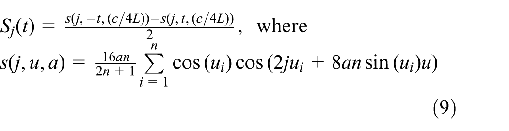
This means that we can express $S_j(t)$ as a difference between a backward and a forward moving waves as

$$\begin{array}{c}{S}_j(t)=\frac{s(j,-t,(c/4L))-s(j,t,(c/4L))}{2},\mathrm{where}\hfill \\ \multicolumn{1}{c}{s(j,u,a)=\frac{16\mathrm{an}}{2n+1}\sum _{i=1}^n\cos (u_i)\cos (2j{u}_i+8\mathrm{an}\sin (u_i)u)}\end{array}$$

(9)

Therefore

$$\begin{array}{c}{q}_j(t)=\frac{g_f(j,t,(c/4L))+g_b(j,t,(c/4L))}{2}+\hfill \\ \multicolumn{1}{c}{\sum _{i=1}^n{V}_{\mathrm{ji}}{A}_i\sin ({\omega }_{i}t+B_i),\mathrm{where}}\\ \multicolumn{1}{c}{g_f(j,t,a)=-s(j,t,a{)*}_{t}Q(t)\mathrm{and}}\\ \multicolumn{1}{c}{g_b(j,t,a)=s(j,-t,a{)*}_{t}Q(t)}\end{array}$$

(10)

This means that if we disregard the effects that are induced by the initial conditions, $q_j(t)$ can be represented by a sum of a forward and a backward moving wave.

Step response

In order to understand how the rod is affected by sudden changes, the step response is investigated. In particular, we investigate a system which is initiated by a steady state where $\mathit{q}=\stackrel{·}{\mathit{q}}=\mathit{x}=\stackrel{·}{\mathit{x}}=0$ . With these initial conditions, all $A_i\mathrm{s}$ in equations (8) and (10) are equal to zero. At time zero, $Q$ is moved to 1, that is

$$\begin{array}{c}Q(t)=\{\begin{array}{cc}0\hfill & \mathrm{for}t<0\hfill \\ \multicolumn{1}{c}{1}& \mathrm{for}t\ge 0\hfill \end{array}\hfill \end{array}$$

The full solution involves computing $g_f$ and $g_b$ from equation (10) as

$$\begin{array}{c}{g}_f(j,t,a)=\frac{2}{2n+1}\sum _{i=1}^n\frac{\cos (2j{u}_i)}{\tan (u_i)}-\hfill \\ \multicolumn{1}{c}{\frac{2}{2n+1}\sum _{i=1}^n\frac{\sin (2j{u}_i+8\mathrm{an}\sin (u_i)t)}{\tan (u_i)}\mathrm{and}}\\ \multicolumn{1}{c}{g_b(j,t,a)=\frac{2}{2n+1}\sum _{i=1}^n\frac{\cos (2j{u}_i)}{\tan (u_i)}-}\\ \multicolumn{1}{c}{\frac{2}{2n+1}\sum _{i=1}^n\frac{\sin (2j{u}_i-8\mathrm{an}\sin (u_i)t)}{\tan (u_i)}}\end{array}$$

The first terms in the expressions are basically Riemann sums and they can be approximated by

$$\frac{2}{2n+1}\sum _{i=1}^n\frac{\cos (2j{u}_i)}{\tan (u_i)}=\frac{2}{\pi }\underset{0}{\overset{\pi /2}{\int }}\frac{\cos (2\mathrm{ju})}{\tan u}\mathrm{du}$$

We have found it difficult to solve this integral for any $j$ although it seems that the integral is equal to one. We have proven this by taking another route to compute $g_f$ and $g_b$ .

In the other route, we compute $Q(t){*}_t{S}_j(t)$ from equation (8) directly. This means that the full solution is

$$\begin{array}{c}{q}_j(t)=\sum _{i=1}^n\frac{k{V}_{\mathrm{ji}}{V}_{1i}}{{\omega }_i^2}(1-\cos ({\omega }_{i}t))\hfill \end{array}$$

for $t$ larger than zero. By noting the fact that ${\mathbf{K}}^{-1}={\mathbf{V}}^T{\mathbf{D}}^{-1}\mathbf{V}$ , we see that $\sum _{i=1}^n\frac{V_{\mathrm{ji}}{V}_{1i}}{{\omega }_i^2}=({\mathbf{K}}^{-1}{)}_{j1}=k^{-1}$ . The inverse of $\mathbf{K}$ can be found in Hovda. ¹³ Therefore

$$q_j(t)=1-\sum _{i=1}^n\frac{k{V}_{\mathrm{ji}}{V}_{1i}}{{\omega }_i^2}\cos ({\omega }_{i}t)$$

(11)

From the analytical expressions for the eigenvectors and eigenvalues, we see that

$$\frac{k{V}_{\mathrm{ji}}{V}_{1i}}{{\omega }_i^2}=\frac{2\sin (2j{u}_i)}{(2n+1)\tan (u_i)}$$

and the step response is therefore

$$q_j(t)=1-\frac{2}{2n+1}\sum _{i=1}^n\frac{\sin (2j{u}_i)\cos ((2\mathrm{cn}/L)\sin (u_i)t)}{\tan (u_i)}$$

Therefore, the forward and the backward moving waves are

$$\begin{array}{c}\multicolumn{1}{c}{q_j(t)=\frac{g(j,(\mathrm{ct}/4L))+g(j,-(\mathrm{ct}/4L))}{2},\mathrm{where}}\\ \multicolumn{1}{c}{g(j,u)=1-\frac{2}{2n+1}\sum _{i=1}^n\frac{\sin (2j{u}_i+8n\sin (u_i)u)}{\tan (u_i)}}\end{array}$$

(12)

In the next section, we will describe $g(j,u)$ in more detail.

The Gibbs-like phenomenon

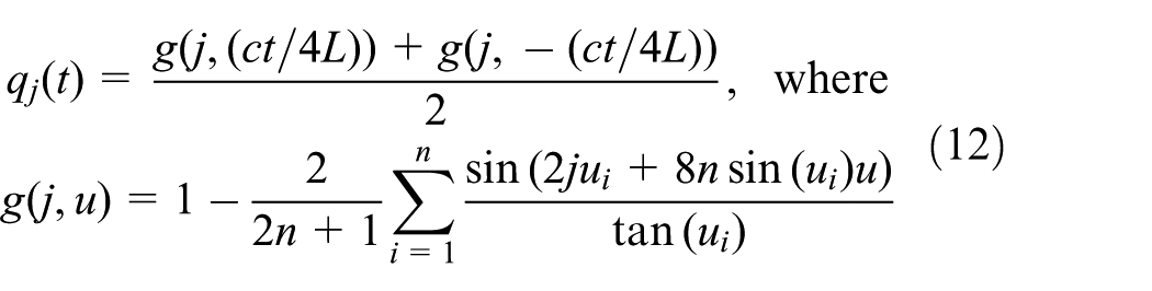
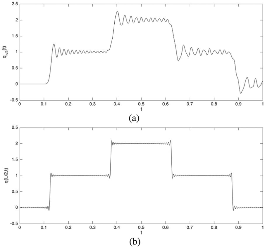
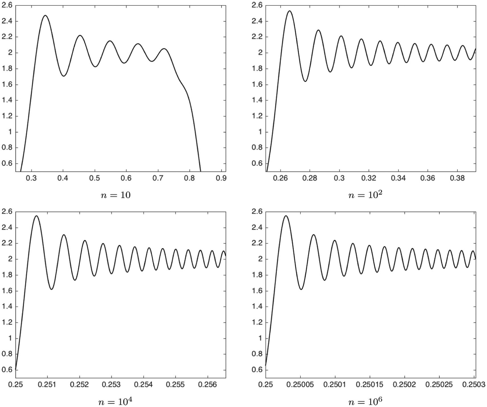
An overview of the behavior of the expressions in equation (12) is illustrated in Figures 4–6. Figure 4 shows one period of $g(j,t)$ for various $j$ when $n=60$ . For large $n$ , $g(j,t)$ is an estimate of the square wave with period one and phase shift $j/(4n)$ . This means that equation (12) is analogous to equation (3). The composition of two oppositely directed waves is illustrated in Figure 5(a), while the analogous Fourier expansion is plotted in Figure 5(b).

Figure 4.

One period of $g(j,t)$ for various $j$ is shown when $n=60$ . The waves are almost identical and $j/4n$ represents the “phase shift” of the wave. The quotes are used because the waves are not perfectly periodic. Similar to the Gibbs phenomenon, the wave includes overshoots and undershoots followed by ringing. However, the Gibbs phenomenon involves an undershoot before the upward step and also an overshoot before the downward step. This effect is not seen in this figure. Moreover, for the same $n$ , the ringing has a lower frequency than the ringing in the Gibbs phenomenon (Figure 1).

Figure 5.

(a) One “period” of $q_{n/2}(t)$ , where $n=60$ . The staircase pattern from Figure 3 is easily recognized. For comparison, $q(L/2,t)$ is plotted in (b), where $f_{\mathrm{sq}}(t)$ is approximated by a partial Fourier expansion with $n=60$ .

Figure 6.

Ten “periods” of $g(n,t)$ , with $n$ equal to 60. It is clear the wave is not fully periodic and that the wave is getting distorted with time.

In Figure 6, we see that after several periods $g(n,t)$ becomes more and more distorted. Clearly, $g(j,t)$ seems to have a “period” of approximately one although it is clear that it is not periodic by the mathematical definition. This can also be understood from equation (12). If we neglect the constant, we see that $g(j,u)$ is a weighted sum of sine waves with different frequencies and phase shifts. Since $u_1\approx \sin u_1$ for large $n$ , we recognize that the sine wave with the lowest frequency is in the scale of $2n/(2n+1)$ .

It is clearly of interest to investigate what happens to $g(n,t)$ for very large $n$ . The most elegant way to proceed is to look at $\underset{n\to \infty }{lim}g(n,t)$ , but unfortunately this has proven to be hard. The terms inside the summation are inherently dependent on $n$ and it is not possible, at least to our understanding, to get out of this dependence. We are therefore restricted from using the plethora of convergence tests that are available for series.

Another approach is to manipulate sum into a Riemann sum, which is a numerical approximation of an integral. The $u_i\mathrm{s}$ goes from approximately 0 to $\pi /2$ and $u_i-u_{i-1}$ is $\pi /(2n+1)$ . This is encouraging, but the $n$ dependence inside the sine wave seems difficult to deal with. Based on this discussion, we leave the attempts of finding analytical expressions for this limit as an open problem.

In the rest of this section, we will describe numerically what is the value at the step, the overshoots and undershoots and the frequency of the ringing. Finally, we will also comment on what happens if we are computing the eigenvalue decomposition numerically.

The value at the step

In Hewitt and Hewitt, ⁹ it is shown that the value at the step of the partial Fourier expansion of the square wave is exactly on the midway between the top and bottom amplitudes as $n$ goes to infinity. We investigate our wave by plotting the value of $g$ as a function of $n$ at the upward and downward steps in Figure 7(a) and (b), respectively. We identify the upward step at $1/2-j/(4n)$ and the downward step as $1-j/(4n)$ . The figures indicate that the value at the step converges to fixed values. For instance, the value of $g(1,1/4)$ is equal to 0.6615 and $g(1,3/4)$ is equal to 1.3415, when $n$ is 10⁷. This indicates that the value at the upward and downward step converges to one-third and two-thirds, respectively, of the jump itself. The fact that this converges for very large $n$ , strengthens the conception of $j/(4n)$ as a “phase shift.”

Figure 7.

The figure shows $g$ at the (a) upward and (b) downward steps as a function of the logarithm of $n$ . When $n$ is small, the curves deviate for different $j\mathrm{s}$ , but when $n$ goes to infinity, the value at the upward step tends to 2/3 and the value at the downward step tends to 4/3.

The level of the overshoot

In order to compute the overshoot, we need to find the first maximum after the step. There is a challenge with using standard numerical methods for finding the overshoot as we need to make initial guesses that are close enough to the local maximum. This is a problem since the frequency of oscillations increases for increasing $n$ .

Our first approach was to use the time at the step as the initial guess and the overshoot was easily detected for small $n$ , but this method became unstable as $n$ increased. We found a practical solution, as we realized that the time from the step to the maximum overshoot $t_{\mathrm{overshoot}}$ is on the order of $a{n}^b$ . By making some rough estimates for $a$ and $b$ , we found small intervals where it was easy to find the maximum values for larger $n$ as well. Finally, we refined the estimates of $a$ and $b$ and ended up with this rule of thumb

$$\begin{array}{c}{t}_{\mathrm{overshoot}}=0.3194n^{-0.6727}\hfill \end{array}$$

(13)

On a log scale, this is a straight line which is plotted together with the estimates in Figure 8(a). The actual overshoot is plotted for various $n$ in Figure 8(b). The two last estimates are equal to 0.5486, which indicates that the actual overshoot is 27.43% of the actual step. The exact same level is seen in the undershoot right after the downward step.

Figure 8.

(a) The time after the upward step for overshoot on a log scale for various $n$ . The line shows the rule of thumb, which is estimated from the two last measurements. Although the estimates do not follow the line for small $n$ , it is clear that the estimates converge to a straight line as $n$ increases. (b) The actual overshoot which seems to converge to 0.5486. This is equivalent to 27.43% of the actual step.

The frequency of the ringing

In order to discuss the frequency of the ringing, we have decided to plot $g(n,t)$ on the domain $[1/4,1/4+10·t_{\mathrm{overshoot}}]$ . This is shown in Figure 9. These results indicate that there is an underlying time scale proportional to $n^{-0.6727}$ which describes the ringing. It follows that the energy of the ringing goes to zero as $n$ goes to infinity, even though the overshoot level remains constant. This is analogous to the Gibbs phenomenon.

Figure 9.

This figure shows $g(n,t)$ as a function of time on the interval $[1/4,1/4+10·t_{\mathrm{overshoot}}]$ for various $n$ . Notice that the plots are similar when the time scales are manipulated in this way. The plots seem to differ less as $n$ increases. This indicates that the energy in the artifact goes to zero as $n$ goes to infinity. It is also worth noting that the frequency of the ringing (wave top to wave top) seems to slowly increase.

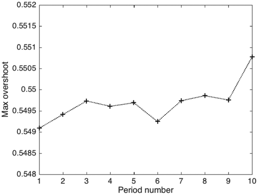
In Figure 10, we see that the overshoot level seems fairly constant from period to period.

Figure 10.

The overshoot in different “periods” for $n=6$ .

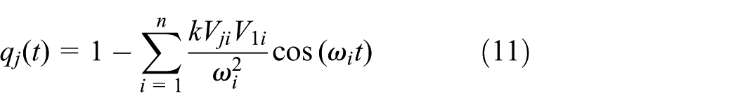
Numerical eigenvalue decomposition

We have two ways to compute $q_j(t)$ . The analytical approach that is given by equation (12) or we can use numerically computed eigenvalues and eigenvectors in equation (11). We call this estimate $q{\prime }_j(t)$ . In Figure 11(a), we have plotted the difference of $q_n(t)$ and $q{\prime }_n(t)$ as a function of time. The error is small, but seems to increase with time. This can be interpreted from equation (12), which is a sum of sine functions. Time is a parameter that is proportional to the frequency of the sine functions. Therefore, when $t$ increases, the sine wave is oscillating with a higher and higher frequency and this becomes more and more difficult to handle numerically.

Figure 11.

(a) Difference between $q_n(t)$ and $q{\prime }_n(t)$ as a function of time and (b) difference between $q_n(1.25)$ and $q{\prime }_n(1.25)$ as a function of n on a log scale.

In Figure 11(b), the difference between $q_n(1.25)$ and $q{\prime }_n(1.25)$ is computed for different $n$ . The time equal to 1.25 is chosen because this is related to the upward step on the second period. The difference increases with $n$ , which can be understood by the impact of $n$ on the frequency of the sine wave. However, note that this difference is still small compared to the ringing effects that are illustrated in this article.

Regularized step function

We are now interested in seeing how the solution is affected using a regularized step function of the form

$$\begin{array}{c}Q(t)=\frac{1}{2}+\frac{1}{\pi }\arctan (\mathrm{Bt})\hfill \end{array}$$

(14)

where $B$ is a parameter that defines the steepness of the step. This function is shown in Figure 12 for $B=100$ and $B=1000$ . We choose the period $a$ to be one and compute $g_f(n,t,1)$ by equation (10). We still consider a system which is initiated by a steady state where $\mathit{q}=\stackrel{·}{\mathit{q}}=\mathit{x}=\stackrel{·}{\mathit{x}}=0$ , that is, all $A_i\mathrm{s}$ in equation (10) are equal to zero. The convolution is computed numerically and $g_f(n,t,1)$ is shown in Figures 13 and 14 for various $n$ . In Figure 13, we use $B=100$ , while in Figure 14 we use $B=1000$ .

Figure 12.

Step functions with various steepness parameters $B$ . The bottom plot is zoomed in on the top part of the step.

Figure 13.

This figure shows $g_f(n,t,1)$ , where the step function has steepness $B=100$ , for various $n$ . The effect of ringing is increasing with time, but seems to disappear with larger $n$ . It is also worth noting that this wave looks like a square wave with rounded corners.

Figure 14.

This figure shows $g_f(n,t,1)$ , where the step function has steepness $B=1000$ , for various $n$ . The effect of ringing is increasing with time, but seems to disappear with larger $n$ . Compared to the case of $B=100$ in Figure 13, the wave is more “square” and a larger $n$ is required to get rid of the ringing.

The method of reducing the Gibbs phenomenon, using a high $n$ in combination with a regularized step function, is somewhat analogous to reducing or eliminating the Gibbs phenomenon using a limited number of Fourier coefficients Barkhudaryan et al. ¹⁴

Conclusion

The mass-spring model is compared to the distributed parameter model on a homogeneous rod, where the left side is subject to a step response, while the right side is free to move. It has been shown that the solution is a sum of a forward and a backward moving wave. In the limiting case when the number of elements goes to infinity, the solutions are likely the same.

However, for a finite number of elements in the mass-spring model, a Gibbs-like phenomenon is observed. The result is an imperfect square wave that is getting more and more distorted with time. At each upward step and at each downward step, the wave seems to overshoot and undershoot to a fixed amount. Different from the Gibbs phenomenon, there is no undershoot before the upward step and no overshoot before the downward step. From a practical point of view, it is promising that using a continuous step function and enough elements in the model, the overshoots, undershoots, and ringing seem to disappear.