
Abstract
Support vector machine has been shown to be an effective classification tool for reliability analysis. Its training set governs the computational cost of the whole reliability analysis. To reduce this training set, researchers focus on important region to decrease samples and refine support vector machine adaptively. In accordance with this methodology, this article presents a more efficient algorithm from the aspect of sampling strategy and that of adaptive manner. To reduce simulated samples, only the important region is considered using Monte Carlo samples in only that region. Moreover, Hasofer–Lind reliability index and the physical meanings of random variables are utilized to identify samples. To speed up convergence of the adaptive procedure, it is proposed to add the most likely support vector to the training set at each step. The illustrative examples show that the proposed sampling strategy largely reduces the classification burden of support vector machine, and the new adaptive procedure converges quickly. The results of the examples demonstrate the proposed method to be accurate and efficient.
Introduction
Estimation of the probability of structural failure is a fundamental task in structural reliability analysis. Essentially, this probability is a multifold integral of joint probability density function of the random variables over the failed domain, that is,
Simulation methods have received much attention from the research community for the assessment of above integral. The fundamental one, Monte Carlo simulation (MCS), samples entire design space according to the joint probability density function. It is rather robust but has to simulate a large number of samples for problems with small failure probabilities. 3 Each sample needs to be evaluated on the performance function, where a time-demanding structural analysis is performed. To alleviate simulation burden, many improved sampling ways are developed, for example, Importance Sampling, stratified sampling, 4 directional sampling, 5 and subset simulation. 6 Among them, Importance Sampling receives most attention from the research community as it can largely reduce samples by focusing only on important region which carries major failure probability content. On the other hand, the original performance function is replaced by an explicit and analytical surrogate model so that structural analysis is then no longer needed. Earlier surrogates in this field are known as response surfaces.7,8 However, they lack flexibility because of the fixed regression model and are strongly dependent on the experimental design. 9 Artificial neural networks 10 and Kriging 11 are also two surrogates used in this field. The former has the issue of local minima and its structure is difficult to determine. 10 And the latter has the difficulty to find suitable theta value. 11 More recently, developments in the field of statistical learning brought a flexible and powerful tool known as support vector machine (SVM). 12 It is constructed according to the principle of “Structural Risk Minimization,” which guarantees a small generalization error. Another advantage is that SVM approximates sign of the performance function directly, not through its value whose approximation requires more computational efforts.
A surrogate is built based on a training set, which consists of points that have been evaluated on performance function. Then, size of training set governs the computational cost of a surrogate-based reliability approach. So, after Hurtado and Alvarez 13 introduced SVM to the field of structural reliability, works on this topic turned to reduce the training set of SVM. Researchers commonly combine the focus on important region and the use of surrogate, for example, SVM. For example, Hurtado and Alvarez 14 use particle swarm optimization to obtain training points in important region, whereas Dai et al. 15 use adaptive Metropolis algorithm to draw training points in the region of most interest. Recently, Alibrandi et al. 16 explore important region by means of sampling cone(s), where training points are generated. Richard et al. 17 propose the rotated star experimental design for SVM regression and adaptively move its position to important region. Also, training points can be reduced according to the fact that only training points closest to the separating hyperplane of SVM contribute to the SVM. Upon this consideration, Jiang et al. 18 take sample pairs (two close samples with different signs and given by a simple nonlinear finite element analysis) as basic elements of training set to reduce useless training points. Moreover, SVM is expressed as a linear combination of functions, each of which is centered on a training point and has only local activation. This flexible structure suggests an adaptive construction procedure where the latest updated SVM is used to guide the selection of new training point(s). In fact, in above works of Hurtado and Alvarez, 14 Dai et al., 15 and Alibrandi et al., 16 SVM is built adaptively. But in their works, new training points are just newly generated samples according to a fixed sampling function. The corresponding adaptive construction procedures are less aimed at SVM accuracy than the suggested one. Basudhar chooses a new sample point that is likely to modify the current SVM and solves the associated problem of SVM locking. The selection is upon multiple considerations and implemented with genetic algorithm.19,20 Hurtado, 21 at each step, evaluates a sample in separation margin of current SVM and then updates current SVM. The samples are generated by Importance Sampling. So, the approach combines focusing on important region and constructing SVM adaptively under guidance of intermediate SVM. However, the training points are selected more or less arbitrarily as more than samples lie in the margin. Bourinet et al. 22 proposed another adaptive scheme where new training points at each step include cluster centers, points in unstable zones and in the margin. This adaptive scheme is designed specially for subset simulation, and the number of training points added in each simulation step is more than 150.
In this article, an explicit criterion for training point selection is proposed with the expectation of most significant improvement in current SVM. The proposed method considers only the specified important region by simulating only Monte Carlo samples in that region. It will be seen that, with this sampling strategy, an important number of samples can be classified directly and effortlessly. And parameter of the sampling strategy is easily determined, which is not the case when Importance Sampling is used.
Principle of SVM for binary classification
SVM is a kind of machine learning method for pattern recognition. It is established according to the rule of structural risk minimization.23,24 As a result, it generalizes well even when established with a small training set.
First, the linearly separable case is considered. A binary classification problem is to determine a hyperplane to separate the given training points. With the aim of structural risk minimization, the hyperplane has to maximize separation margin, which is the shortest distance from training points to separating hyperplane. Assume that the training set contains m points in n-dimensional space,

in which
Noticing that equation (1) is invariant by positive rescaling, the condition

This constrained optimization problem satisfies the Karush–Kuhn–Tucker conditions. So, it could be converted to a dual problem, which is easily handled. The corresponding Lagrange function is first constructed

where
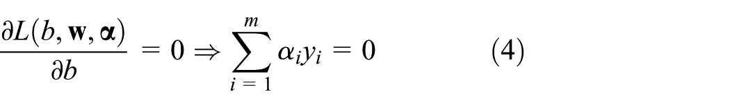
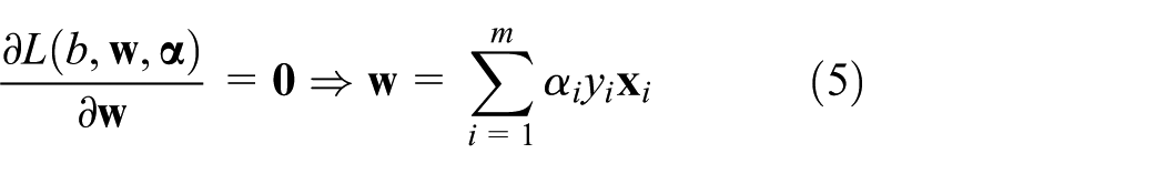

In addition, one of the Karush–Kuhn–Tucker conditions is

Substitution of equations (4) and (5) into equation (3) yields
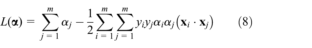
As the desired

This equation would provide the solution of

in which
It is noteworthy that equations (5) and (7) are of great significance. Equation (7) indicates that either
Next, we consider the general case where linear separation is impossible. The basic idea to deal with this case is to map training points to a higher dimensional space by a nonlinear projector

in which the parameter
The proposed method
Like FORM (first-order reliability method) and Hurtado’s 21 method, the proposed method aims to solve low-dimensional problems with unique MPP (or comparative MPP, MPP is short for most probable failure point). For this type of problems, probability density decays exponentially with the distance from origin in standard normal space. As MPP is the failure point with the largest probability density, most failure probability content concentrates around MPP. This region is thus the important region, which should receive more attention during failure probability estimation. It is noted that, in this case, taking account of the failure probability content only in the important region would not harm the accuracy of the simulated failure probability while largely reducing the samples. In view of this, it is proposed to perform MCS only in that region. Subsequently, to reduce SVM training set, an adaptive scheme is developed with emphasis on criterion for training point selection. According to the geometric interpretation of the MPP, some samples can be identified to be safe, and, if possible, the physical meanings of all the random variables can also be utilized to identify samples.
MCS in important region
Important region is identified by MPP, which should be searched first. MPP search is the fundamental task of FORM. FORM commonly adopts a gradient-based algorithm to search the MPP, and the gradients are calculated by a finite difference scheme. This search algorithm is adopted here. In view of its non-robustness (robustness means a wide scope of application), other search algorithms can be used instead when necessary. Except the search algorithm of FORM, existing search algorithms can at least be found in the works of Dai et al.,
15
Hurtado,
21
which both present Markov chain based algorithm, and Gong et al.,
25
which reports a non-gradient algorithm. Without loss of generality, the important region is specified as a hypercube centered on the MPP and with a range of

Illustration of Monte Carlo simulation in the important region with Example 1.
Next, sampling is performed according to the joint probability density function, but only the samples in the important region are reserved, as shown in Figure 1. When these samples are classified, the conditional failure probability in the important region can be estimated by
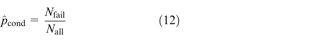
where

where
It is reminded that MPP is the closest failure point to the space origin, indicating that any sample in the β-sphere (as shown in Figure 1,
In engineering context, random variables (e.g. geometry sizes, loads, and material parameters) are usually associated with clear physical meanings which show positive or negative effect on structural safety. With this information, a known point (point with a known class) can be used to identify unknown points in the same class as itself. To be specific, an unknown point can be inferred to be safe if it has larger geometry sizes, larger material parameters, and lower loads, compared with a known safe point; on the contrary, given a failure point, points meeting the opposite conditions simultaneously are judged to be failed. It needs to be emphasized that this identification can be carried out only if all of the random variables express a deterministic effect on structural safety. Clearly, the use of β-sphere and physical meanings of all the random variables would play a less important role for higher dimensional problems.
Adaptive scheme to build SVM
Sampling is performed in standard normal space, which is obtained by transformation of original design space. However, this transformation increases nonlinearity of the limit state surface. 9 This is especially detrimental for the use of SVM, which directly approximates the limit state surface. It is thus preferred to classify samples in original space. Note that space transformation does not change the implied effects of random variables on structural safety. Hence, sample identification according to the physical meanings of all the random variables would not be influenced by space transformation.
SVM is applied in original design space. According to the principle of SVM, separating hyperplane is determined by only support vectors. Evaluations of the rest training points are thus a waste of efforts. However, the support vectors can be recognized only when the separating hyperplane is available. As a compromise, an adaptive scheme is devised where the SVM is continually refined by evaluating only the current most likely support vector at each step. At each step, the evaluated sample is used to identify more samples according to the physical meanings of all the random variables if possible. Next, all the newly known samples are added to the training set and then the current SVM is updated. The initial training set of the adaptive scheme can be readily obtained from all the points evaluated during MPP search.
A question that naturally arises is how to measure the likelihood to be a support vector with absence of the exact separating hyperplane. It is adopted here that the measurement is made with the latest updated one, instead. At intermediate steps, the sample
The adaptive scheme is directly aimed at the classification accuracy of SVM on the samples. The convergence condition of the adaptive scheme is further defined by the target of the entire analysis, that is, the failure probability. Once the SVM is updated, a new estimate of the failure probability is given by

in which
Finally, the application of Gaussian RBF kernel during SVM construction needs to be detailed. The SVM toolbox in MATLAB is used to implement the construction of SVM for each training set. Except that the parameter plays an important role, the penalty parameter is commonly introduced to make the SVM model more flexible. To optimize these two parameters, the grid optimization approach is adopted, which is a proven technology. Given a series of candidate values for each parameter, this approach tries all possible combinations and carries out cross-validation for each combination. Finally, the combination with the minimum mean error is adopted. For a careful consideration, the possible ranges of both
Implementation procedure
For the sake of clarity, the whole implementation procedure of the proposed method is presented:
Step 1. Transform original design space to standard normal space by Nataf transformation. 27 In the new space, search MPP as FORM usually does. Points evaluated on the performance function in the search process are reserved.
Step 2. Specify the important region, where Monte Carlo samples are then drawn. The samples in the β-sphere are identified as safe samples directly. Each of the known points, including the safe samples and the evaluated points during MPP search, is used to identify samples according to the physical meanings of all the random variables if possible.
Step 3. Transform the standard normal space back to the original space. Correspondingly, all samples are transformed. Leave out the evaluated points not in the important region and transform the rest.
Step 4. Establish SVM using all the known points and then predict signs of all the unknown samples by the SVM. Subsequently, failure probability is estimated according to equation (14). Afterward, the convergence condition is examined. If it is satisfied, the whole procedure is ended with current estimate of the failure probability as the end result.
Step 5. Choose the unknown sample with the minimum
Example validation
To validate the proposed method, four typical examples are analyzed. Accuracy and computational cost of the proposed method are compared with those of other methods. Among these methods used for comparison, Hurtado’s 21 method is more focused as it deals with the same kind of reliability problems and shares similar methodology with the proposed method. AK-IS (active learning Kriging and Importance Sampling) 28 and Bourinet et al.’s 22 method are considered but not for all the following examples since they are both proposed specially for problems with small failure probabilities. As performance function evaluations govern the computational cost in real engineering context, the number of calls to the performance function (denoted as Ncall below) is used to qualify the computational cost. For all the examples, the proposed method, Hurtado’s method, AK-IS and Alibrandi’s method search MPP by the gradient-based algorithm. They are thus on top of the cost of FORM as MPP search contributes the main computational cost of FORM.
Example 1: two-dimensional nonlinear example
For the sake of graphic visualization, a two-dimensional case is studied first, which is also used for validation in the works by Grandhi and Wang 29 and Grooteman. 30 It has a small failure probability and its nonlinear performance function reads

in which
Results are presented in Table 1. The reference failure probability is obtained by MCS with 1E7 samples. The MPP search starts at the space origin. It just takes six calls to the performance function, offering the MPP and
Results of Example 1.
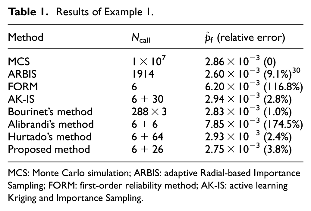
MCS: Monte Carlo simulation; ARBIS: adaptive Radial-based Importance Sampling; FORM: first-order reliability method; AK-IS: active learning Kriging and Importance Sampling.
Figure 2 shows the changes in the failure probability estimate in the proposed adaptive procedure. It can be seen that the estimate quickly reaches a stable stage. Table 1 indicates that the proposed method yields a failure probability very close to the reference value, but with much less computational cost than MCS, adaptive Radial-based Importance Sampling (ARBIS),
30
Bourinet’s method, and Hurtado’s method. Its efficiency may be attributed to the following three aspects. First, as a matter of fact, the probability content of the important region is as little as 0.155. This value implies that the proposed method just needs 0.155 times of samples required by MCS for a similar accuracy level. Second, among the total 1E4 samples, 9413 samples lie inside the β-sphere (see Figure 1), so they can be identified as safe samples effortlessly. Finally, the designed adaptive scheme to build SVM, mainly the criterion for training point selection, makes a fast convergence speed. AK-IS shows roughly equivalent performance with the proposed method under an overall consideration of efficiency and accuracy. Bourinet et al.’s
22
method is most accurate but requires a rather heavy computational burden. When applying Alibrandi et al.’s
16
method, the suggested aperture

Example 1: history of the convergence of the proposed method.
Example 2: dynamic response of a nonlinear oscillator
The second example involves a nonlinear undamped system with single degree of freedom (Figure 3). It has been served as a validation example for many times.31,32 The performance function is defined by

with

The nonlinear oscillator.
Distributions of the random variables in Example 2.

The results of FORM, Hurtado’s method, and the proposed method are shown in Table 3, also shown are two methods combining Importance Sampling and different surrogate,
31
AK-MCS (active learning Kriging and Monte Carlo simulation),
32
AK-IS, and Alibrandi’s method. FORM searches MPP with 21 calls to the performance function and accordingly gives a failure probability with a relative error of 9.1%. Using the MPP, the proposed method decreases the relative error to 4.5%. This is achieved at the expense of additional 32 calls to the performance function. For the same purpose, Hurtado’s method performs additional 56 calls to the performance function and produces a relative error of 4.9%. Alibrandi’s method performs additional 30 calls to the performance function, but the relative error is as much as 31.6%. For the proposed method, the important region is defined by
Results of Example 2 (case 1: mean and standard deviation of F1 are 1 and 0.2, respectively).

MCS: Monte Carlo simulation; FORM: first-order reliability method; AK-MCS: active learning Kriging and Monte Carlo simulation; AK-IS: active learning Kriging and Importance Sampling.
The second case is taken from the work of Echard et al., 28 where mean and standard deviation of F1 are 0.6 and 0.1, respectively. These values are adopted to produce a rather small failure probability. Results obtained by related methods are presented in Table 4. The proposed method applies least computational cost except FORM and its accuracy is satisfactory. In its application, important region is defined as in the previous case and the corresponding probability content of the important region is 0.1478. So, the required samples can be largely reduced compared with MCS. Still, 2E6 samples are used for such a small failure probability. However, most samples are in the β-sphere and the samples remain to be classified are only 4522. So, the role of β-sphere in this case is significant, which contributes largely to the efficiency of the proposed method.
Results of Example 2 (case 2: mean and standard deviation of F1 are 0.6 and 0.1, respectively).

MCS: Monte Carlo simulation; FORM: first-order reliability method; AK-IS: active learning Kriging and Importance Sampling.
Example 3: 23-bar truss
This example deals with a 23-bar truss structure (Figure 4).
33
It includes a moderate number of random variables, which are non-normally distributed. The concerned safety requirement is that the center deflection (


The 23-bar truss structure.
Statistic properties of all the random variables are shown in Table 5. Elastic modulus and cross-sectional areas are assumed to be perfectly correlated among all the horizontal bars, so is the case with all the diagonal bars. In Table 5, E1 and A1 denote the elastic modulus and cross-sectional area, respectively, for all the horizontal bars. For all the diagonal bars, the elastic modulus and cross-sectional areas are E2 and A2, respectively.
Distributions of the random variables in Example 3.

Results are shown in Table 6, where RSMM is the abbreviation for response surface augmented moment method.
33
FORM performs 44 calls to the performance function and gives a failure probability with 40.0% relative error. The proposed method reduces the relative error to 1.1% with additional 32 calls. In this process, 1E3 samples are drawn in the important region specified with
Results of Example 3.

MCS: Monte Carlo simulation; RSMM: response surface augmented moment method; FORM: first-order reliability method; AK-IS: active learning Kriging and Importance Sampling.
Example 4: three-bay and 12-story frame
Finally, a frame structure
34
(shown in Figure 5) is studied based on the consideration that the implied finite element model involves another typical element type, beam element. This structure is assumed to have six basic random variables, which are the wind load P, the member cross-sectional areas A1, A2, A3, A4, and A5, respectively. Ai corresponds to the members labeled with number i (see Figure 5),

in which

The three-bay and 12-story frame structure.
Distributions of the random variables in Example 4.

The performance function is defined as

where
Results of this example are listed in Table 8. The reference failure probability is obtained by Importance Sampling with 2000 samples.
34
Two surrogate-based simulation methods are also included for comparison.10,35 It can be seen from Table 8 that FORM needs least performance function evaluations but is inaccurate. The cumulative formation of response surface and Alibrandi’s method require not too much cost but their relative errors are large. On the contrary, the RBF network requires much more cost but yields almost exact result. An accurate result is also achieved by the proposed method. But only two times of the calls to the performance function are needed in comparison with FORM. For this example, the important region is defined by
Results of Example 4.

FORM: first-order reliability method.
Discussion
AK-IS cannot be as efficient as the proposed method for this ten-dimensional example (Example 3). And it is specially designed to cope with small failure probabilities, which, however, may not be easily identified beforehand in practical case. Alibrandi’s method can be considered as efficient, but it is hard to guarantee the accuracy of the result. On the contrary, Bourinet’s method gains accurate result with large computational cost.
The proposed sampling strategy consists in restricting MCS in the important region so that samples can be reduced. From the other side, the failure probability content outside the important region will not be counted in the failure probability integral. So, the side length of the important region k should be large enough to cover most failure probability content. However, increase in k results in more samples to be simulated. It is clear that there is a trade-off between preserving accuracy and improving efficiency. In section “MCS in important region,” the interval [1, 2] is recommended based on more or less experience. It is applicable for all the examples except the second one. In view of this, one can set the value of k adaptively when necessary. One can start with a small k and then increase it for several times until the failure probability stabilizes. Each k is associated with a complete estimation process for the failure probability. During each estimation, sampling is started from the same seed so that samples in previous estimation can be reused. Therefore, the adaptive way will not bring substantial increment of computational cost than the direct assignment of k. To illustrate the adaptive way, the second example is reanalyzed where k is adaptively determined. The variation in the results due to the changes in k is obtained, which is shown in Figure 6. Figure 6 indicates that the adaptive way is applicable.

Example 2: effect of size of the important region on the results of reliability analysis.
Also concerned is the sample amount, which is determined by the conditional failure probability of the important region for a given accuracy level. In above examples, we set a whole number directly with a coefficient of variation of the failure probability between 0.05 and 0.1 just to show the performance of the proposed algorithm. As the conditional failure probability is the goal of the simulation in practical applications, an adaptive way is suggested to determine the sample amount when prior knowledge about the conditional failure probability is not enough. Its implementation is quiet simple. First, a small number of samples are generated. Then, conditional failure probability is estimated, according to which the required number is recomputed. Sampling is then continued to reach the required number, which initiates the next cycle of estimation. In general, both the sample amount and the conditional failure probability would converge after several steps.
Finally, to validate the efficiency of only the proposed criterion for training point selection, we compare the proposed criterion with that of Hurtado’s method, which selects a sample in the SVM separation margin at each step. To this end, the corresponding two adaptive schemes are executed with respect to the same sample population and from the same initial training set. The β-sphere and the physical meanings of random variables are not considered here. Example 3 is taken for the validation. Sample population and initial training set are those adopted by the proposed method in Example 3. The numbers of additional calls to the performance function for the proposed scheme and Hurtado’s scheme are 29 and 73, respectively. The results indicate that the proposed criterion for training point selection is more efficient than that of Hurtado’s method.
Conclusion
Regarding the use of SVM in reliability analysis, several papers have proved that it is efficient to iteratively refine SVM with focus on important region. This article applies SVM in the same way for low-dimensional problems with unique MPP. Its originality mainly lies in two aspects. First, simulation is only for the important region and Monte Carlo samples in that region are used. Second, for the adaptive scheme to build SVM, a criterion for training point selection is proposed which adds the most likely support vector to the training set at each step. The examples indicate that the proposed sampling strategy can largely reduce the samples to be classified with the consideration of the geometrical interpretation of Hasofer–Lind reliability index β. Moreover, physical meanings of all random variables are utilized to identify samples if possible. The criterion for training point selection can speed up the convergence of the adaptive procedure for SVM construction compared with Hurtado’s method. The four typical examples prove that the proposed method is accurate and efficient. For a more flexible method, the important region and the sample amount can be specified in an adaptive manner without a significant increase in computational cost.
Footnotes
Academic Editor: Jianqiao Ye
Declaration of conflicting interests
The author(s) declared no potential conflicts of interest with respect to the research, authorship, and/or publication of this article.
Funding
The author(s) disclosed receipt of the following financial support for the research, authorship, and/or publication of this article: This work was supported by the Fundamental Research Funds for the Central Universities (Grant No. HIT.MKSTISP. 201609).