
Abstract
The effects of uncertainties on the nonlinear dynamics of complex structures remain poorly mastered and most methods deal with the linear case. This article deals with a model of a large and complex structure with uncertain parameters for the nonlinear dynamic case, and the reduction in the model discretized by the finite element method is obtained by reducing the degrees of freedom in the numerical model. This is achieved by the development of the unknown displacement vector on the basis of the eigenmodes; a particular attention is paid to the calculation of the nonlinear stiffness coefficients of the model. The method combines the stochastic finite element methods with a modal reduction class based on sub-structuring the component mode synthesis method. The reference method is the Monte Carlo simulation which consists in making several simulations for different values of the uncertain parameters. The simulation of complex and nonlinear structures is costly in terms of memory and computation time. To solve this problem, the perturbation method combined with the component mode synthesis reduction method significantly reduces the computational cost by preserving the physical content of the original structure. The numerical integration by the Newmark schema is used; the first statistical moments (mean and variance) of the nonlinear dynamic response are computed. Numerical simulations illustrate the accuracy and effectiveness of the proposed methodology.
Keywords
Introduction
In a robust design process, the determination of the variability of the nonlinear dynamic response of a large and complex structure is essential. Uncertainties come from the tolerances of manufacturing, the boundary conditions, and the external excitations. These structures are largely used in the fields of aerospace, automotive, civil engineering, and so on.
The uncertainty of the physical parameters, nonlinearity, and complexity of the structure require the development of a complete mathematical approach for predicting the dynamic behavior variability.
In addition, several methods have been developed in the literature to take account of uncertain parameters in the nonlinear dynamic response.
The reference method is the Monte Carlo simulation. 1 This method allows a statistical evaluation based on a large number of deterministic analyses by considering different values of uncertain parameters. However, it requires the generation of big size samples and then generates a prohibitory time computing. This approach is thus very costly.
Also, perturbation methods are widely used to calculate the first moments (mean and standard deviation) of dynamic response whose uncertain variables vary slightly. These techniques are based on the Taylor series development of the response around its mean. This allows the direct determination of the variability of the response according to the physical parameters (mechanical and geometrical) randomly.
Indeed, perturbation methods based on a development in Taylor series of second order 2 and Neumann expansion method 3 are generally efficient. Another development in the first order 4 gives a similar result to the previous developments with a reduced time computing. Recently, in the field of thermal conduction with uncertain parameters,5–7 combination of a probabilistic study based on the perturbation method with a numerical resolution based on the finite difference method is applied. 5 A prediction of the temperature field with random and fuzzy parameters of the properties of materials is studied; a numerical technique called fuzzy stochastic finite element method based on the combination of the perturbation theory with the moment methods is adopted. 6
Furthermore, another form of development is a polynomial chaos expansion (PCE).8,9 The stochastic solution may be expanded in terms of the polynomial chaos basis whose elements are obtained from orthogonal polynomial. 10 The properties of this polynomial basis are used to generate a system of deterministic equations. The resolution of this system is used to determine the variability of the response.
However, nonlinear dynamics, the large number of degrees of freedom (DOFs) due to the mesh of a large structure, and higher order developing for modeling uncertainty induced a considerable increase in deterministic equations.
One way to solve this problem is the reduction by component mode synthesis (CMS) method proposed in the literature.11–18 This method allows condensing the large number of DOFs into a small number using the generalized coordinates. FA Lulf et al. 19 proposed a comparative study of different bases for reduction in nonlinear dynamic structures. Thus, in the CMS method, the overall structure is divided into sub-structures, each of which is analyzed independently in order to obtain the corresponding solution. These solutions are combined to obtain the overall solution of the structure by imposing constraints on the interfaces. The different methods are classified according to CMS interface: fixed interface, 11 free interface,12,13 or hybrid interface.14,16
Recently, D Sarsri et al.20,21 developed an approach coupling CMS reduction method and developing uncertainty by a PCE to calculate the frequency transfer functions and response temporal for linear stochastic structures. J Sinou et al. 22 proposed for simple structures, requiring no reduction, a technique taking into account the uncertainties in nonlinear models by combining the method of harmonic balance method (HBM) and developing uncertainty by a PCE. This method is based on a formulation of nonlinear dynamic problem in which the physical parameters, nonlinear forces, and the excitation force are considered randomly.
In another work, D Sarsri and L Azrar 23 used the CMS method coupled with the perturbation method to calculate the stochastic modes of large finite element models with uncertain parameters for the linear problems.
This work is an extension to the nonlinear problems. The aim is to estimate the stochastic nonlinear dynamic response for a large structure with a minimum computational cost. To do this, we develop a methodological approach for calculating the temporal response of a large structure with uncertain parameters. This approach is based on coupling of the perturbation method and the reduction (CMS) method. First, we develop the nonlinear dynamic equations considering geometrical nonlinearity. The resolution of the nonlinear dynamic problem by the finite element method is adopted. Then, the temporal integration by Newmark scheme is developed. Second, we take completely the random phenomena using the perturbation method. The method of stochastic finite element is used. Various types of CMS interface method are used to optimally reduce the model size. The first moments of the nonlinear dynamic response of the reduced system are compared with the entire system. Several numerical simulations have shown the accuracy and efficiency of procedures and methodologies developed.
Modeling of nonlinearity
The discretization by the finite element method of a linear structure gives the following matrix system

where
Intermittent contact or friction called nonlinearity of contact modeled by nonlinear force

Large displacement for thin structures called geometric nonlinearity modeled by nonlinear force
The nonlinear system modeling the nonlinear dynamics of a structure discretized by the finite element method is given by

where
CMS reduction method
The CMS method consists in using simultaneously a sub-structuring technique and a reduction method. The large and complex structure is partitioned into sub-structures. Each sub-structure is represented by a reduced basis composed of the normal modes and the interface modes. We present the theoretical bases of the CMS method. Initially, the eigenmodes and the interface static deformations are given for each sub-structure. Then, the overall system is projected on these bases taking into account the interface couplings between the sub-structures, after the reduced system is solved. Finally, the complete system solution is reconstituted.
The finite element model of the entire structure is partitioned into N sub-structures SS(i) (i = 1, …, N). The equations of motion for each nonlinear sub-structure SS(i) are

where
The displacement vector

The external force vector

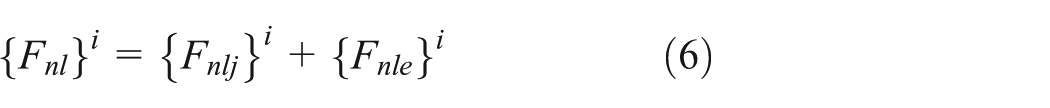
The nonlinear force vector
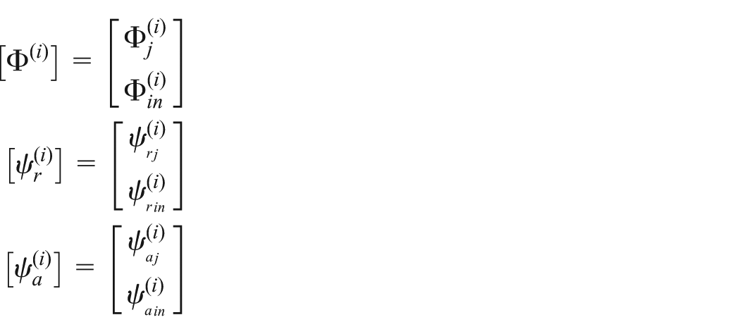
In the CMS methods, the physical displacements of the sub-structure SS(i) are expressed as a linear combination of the sub-structure modes. After some algebraic transformations, a set of Ritz vectors Q is obtained and the displacement vector of each sub-structure can be expressed as

where
1. Free interface method
In the free interface method, the displacements of each sub-structure are expressed as

where

where
The expression of

else
with

and

where
To preserve the interface DOF, the following partition is used
Using this partition, one obtains

The matrix Q is then given by

2. Fixed interface method
In the fixed interface method, the displacements of each sub-structure are expressed as

The matrix

where
The conservation of interface DOF allows assembling these matrices as in the ordinary finite element methods. Let us denote the vector of independent displacements of the assembled structure by

The compatibility of interface displacements of the assembled structure is obtained by writing for each sub-structure SS(i) the following relation

where
A transformation matrix can be defined for each sub-structure SS(i) by

where
The displacement vector

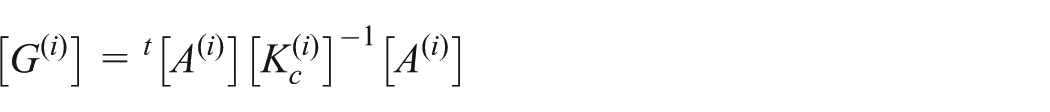
Inserting equation (17) into equation (1) and multiply on the right by

where
Using the interface DOF compatibility of displacements, it can easily be shown that

Finally, the reduced equation of motion can be written as follows

Stochastic perturbation method
The perturbation method is largely employed in the field of the stochastic finite elements. It is based on an approximation the random variables by their development in Taylor series around their average value. These developments are truncated at the second order. The perturbation method must obey the conditions of existence and validity, in particular the reduced field of variation of the random variables. We present an extension of this method for the nonlinear dynamic systems with uncertain parameters.
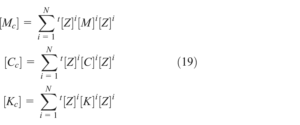
Let us assume that for each sub-structure, the mass matrix
In the time domain, the resulting reduced stochastic differential system equation (21) has to be solved. The first two moments of time response (average and variance) will be calculated using the second-order perturbation method.
One defines the vector of the average parameters
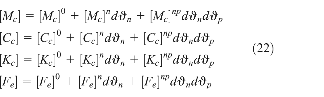
where [.]0, [.]
n
, and [.]
np
are deterministic matrices corresponding to the zero-, the first-, and the second-order partial derivatives with respect to the random parameter

Indicial notations are used, with indices n, p running over the sequence 1, 2, …, I as well as the repeated indices summation.
For structures with small uncertainties, one can assume that the transformation matrix

where
The unknown vector displacement, velocity, and acceleration are also developed through Taylor series as follows

And the vector nonlinear force is given as

Then
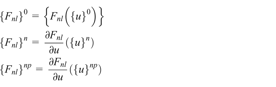
The condensed nonlinear forces are

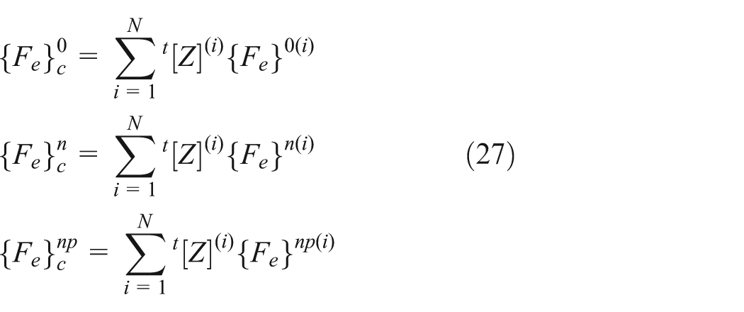
The condensed external forces are
Substituting these developments into equation (21) and writing the terms of same order on gets the following differential systems:
Zero-order equation

First-order equation
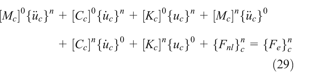
Second-order equation

Stochastic temporal response
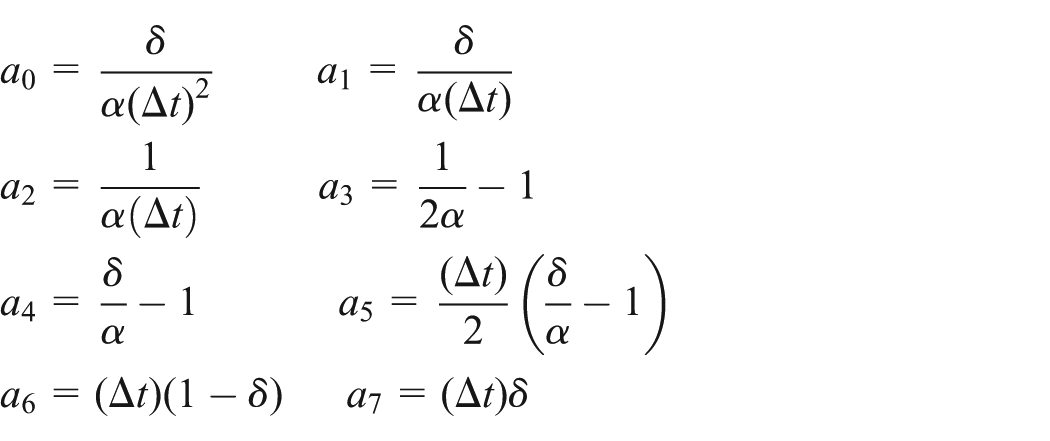
The temporal response from time 0 to time T of equations (28)–(30) is required. The time T is subdivided into n intervals

where x can take 0, n, and np values.
In which, the two parameters
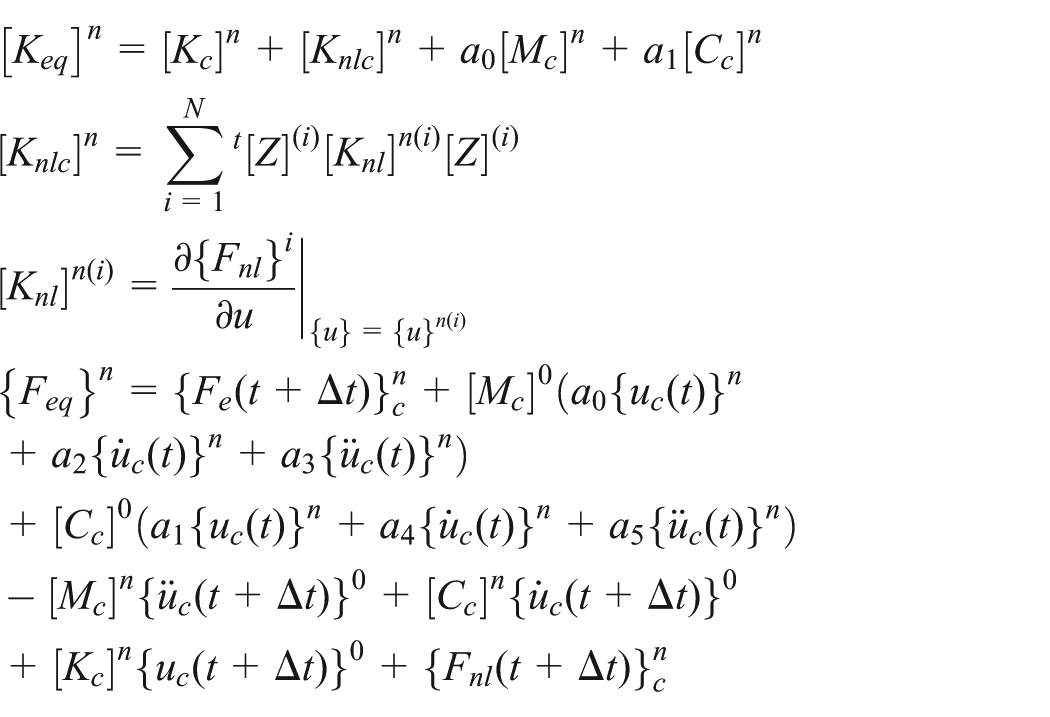
Based on these notations, the following equations are resulted:
Zero-order equation

with

First-order equation

with
Second-order equation

with

The solution of the problem is obtained by successively solving the following algebraic equations

The derivative of the physical displacements of each sub-structure is then obtained by

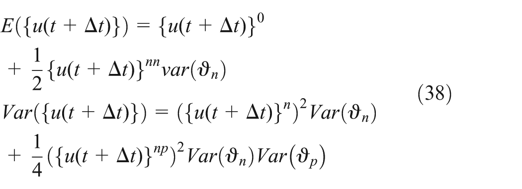
The mean and the variance values of displacement

If the correlation between the random parameters is not considered, equation (37) can be simplified as
Numerical example
For nonlinear discrete systems with stochastic parameters, some benchmark tests are elaborated to demonstrate the efficiency of the methodological approach. The presented method can be applied to continuous or discrete systems. In this article, we restrict ourselves to show the applicability and effectiveness of these methods for the dynamic analysis of nonlinear discrete systems with N DOFs. A nonlinear dynamic system consisting of 20 masses connected by 21 springs nonlinearly is shown in Figure 1. This structure will be divided into two sub-structures SS(1) with 11 internal DOFs and SS(2) with 8 internal DOFs, and 1-DOF of junction the mass m/2. The starting equation 20-DOF will be condensed and will bring to the resolution of a 10-DOF equation, divided into 1 junction DOF, 5 modes free or fixed interfaces of SS(1) and 4 modes free or fixed interfaces for SS(2).

Decomposed structure.
The following characteristics are considered:
Masses:
Linear stiffness:
Nonlinear cubic stiffness:
The initial conditions are
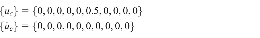
To illustrate the steps of the previously presented method, one begins by writing the vibration of the overall system of equations and those subsystems.
The time responses of the entire system (without reduction) and the system decreased with a fixed interface and free interface (CMS) method are shown in Figures 2–4 which correspond, respectively, to temporal displacements of the mass (12) which corresponds to DOF junction, mass (1) of the sub-structure SS(1), and the mass (18) of the sub-structure SS(2). We can see that the different methods of modal synthesis provide very similar results. Other numerical results were obtained for different types of loading and modal decomposition. Adaptation to the assembled continuous systems is straightforward using the finite element method.

The temporal displacement response for m(12).
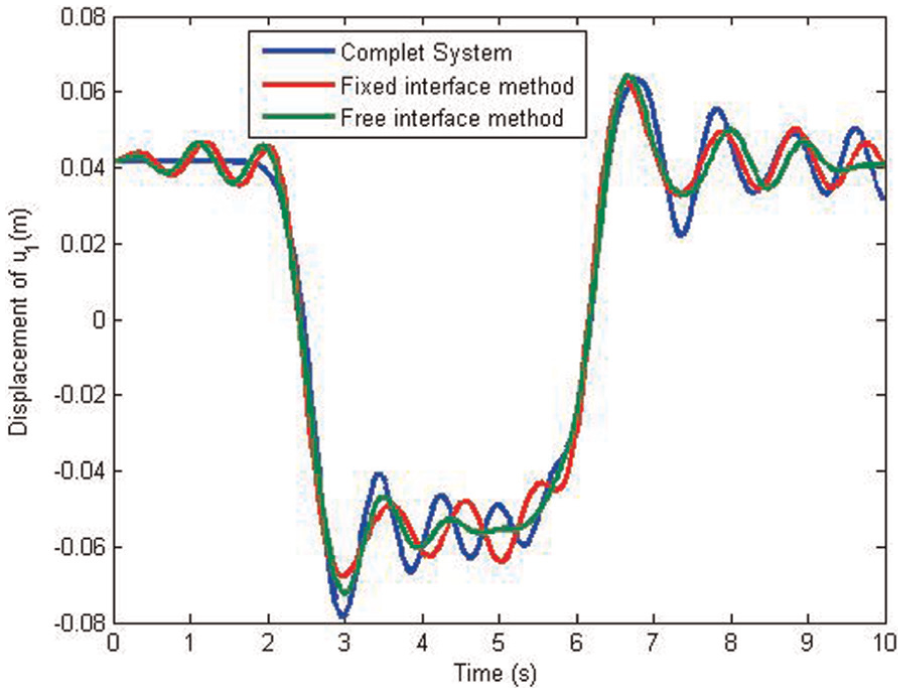
The temporal displacement response for m(1).
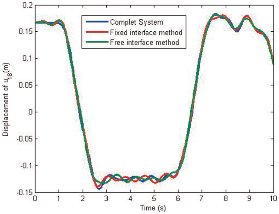
The temporal displacement response for m(18).
In this study, it has been chosen to investigate the effects of uncertainties by considering mass uncertain parameters. The mass parameter is supposed to be a random variable and defined as follows:

(a) The mean of temporal response for m(12) and (b) the variance of temporal response for m(12).

(a) The mean of temporal response for m(1) and (b) the variance of temporal response for m(1).
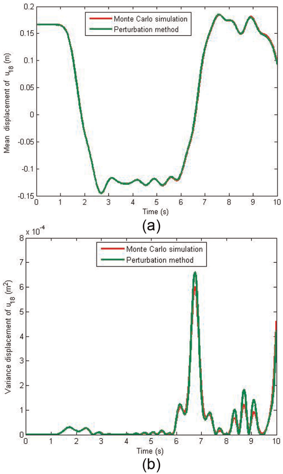
(a) The mean of temporal response for m(18) and (b) the variance of temporal response for m(18).
Finally, we used the approach based on the coupling of the perturbation method with CMS condensation method. This approach allows reducing the size of the problem and the computational cost. The mean and variance of displacement have been shown in Figures 8–11. We can see that the different methods provide very similar results.

The mean of temporal response for m(1), Monte Carlo simulation with 700 samples, and perturbation with whole structure and with free and fixed interface (CMS) methods,

The variance of temporal response for m(1), Monte Carlo simulation with 700 samples, and perturbation with whole structure and with free and fixed interface (CMS) methods,

The mean of temporal response for m(12), Monte Carlo simulation with 700 samples, and perturbation with whole structure and with free and fixed interface (CMS) methods,
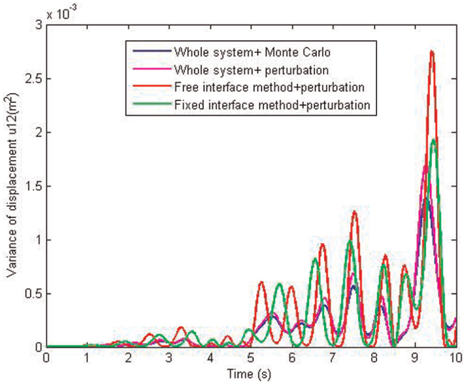
The variance of temporal response for m(12), Monte Carlo simulation with 700 samples, and perturbation with whole structure and with free and fixed interface (CMS) methods,
Conclusion
The main aim of this work is to provide the variability of the transient solution of a large and complex structure by considering geometric nonlinearities. We have achieved this by implementing an integrated approach, the coupling perturbation method, CMS reduction method, and temporal integration. The perturbation method was used to model the uncertain parameters by a development in Taylor series of second order. We developed the CMS method in the nonlinear case for reducing the finite element model. The implementation of the temporal integration by Newmark schema has allowed us to establish the variability of the solution for nonlinear reduced model with uncertain parameters. We could solve the problem of calculating the tangent matrix. The numerical tests show the accuracy of the results and minimization of cost calculation, thus validating this approach.
Footnotes
Academic Editor: Luís Godinho
Declaration of conflicting interests
The author(s) declared no potential conflicts of interest with respect to the research, authorship, and/or publication of this article.
Funding
The author(s) received no financial support for the research, authorship, and/or publication of this article.