Sage Journals: Discover world-class research

Abstract

The extraction of coalbed methane, unlike that of conventional gas resources, is characterized by low gas production and low pressure. The traditional optimization methods only focus on the surface system, ignoring the relationship between the surface system and coalbed methane production. Furthermore, the pipeline network suggested by these methods is based on the given productivity of a single well. This article proposes a surface system layout optimization architecture coupled with a production system simulation that considers the profit made in the production cycle as the objective function. Using case studies, we show that the proposed optimization method improves the gas production rate by about 10.9% and increases the profit by 2 million dollars. When the results are analyzed under different network topologies, the tree network emerges as the cheapest and the star network emerges as the most expensive in terms of ground investment. However, when considering productivity and profit, the star network is the best and the tree network is the worst, while the concatenated network is intermediate. The results show that the structure of the surface network has a considerable influence on the coalbed methane reservoirs. Therefore, this article recommends the star structure arrangement for the coalbed methane surface system.

Keywords

Coalbed methane surface network design optimization architecture production system simulation network topology

Introduction

Coalbed methane (CBM) is an important sustainable energy resource. CBM is very abundant in China, where approximately 36.81 trillion cubic meters of CBM exist at a shallow land depth of 2000 m.¹ The generation of CBM is characterized by low production, low pressure, dense wells, and large pressure interference between wells. Furthermore, as its daily production is low, it needs to be continuously extracted on a large scale, resulting in high initial investment costs. As the CBM industry has developed, high CBM gathering and transportation costs, accounting for more than a third of the total costs incurred, have restricted its growth. The design of the surface pipeline system directly determines the parameters and the investment; however, as development in the field of CBM gathering has increased, the economic problem created by surface engineering has also increased. This problem is primarily solved by optimizing the design of the pipeline network. Domestic and foreign researchers have carried out several studies on the optimization of oil–gas pipeline network designs in recent years. Using graph theory, Dijkstra² solved two problems: constructing the shortest tree connecting n nodes and finding the shortest path between two given points. To determine the optimal layout of the oil–gas gathering and transportation main line, Coats³ considered the impact of a single line, multiple lines, and different-sized pipes and then used the geometry method to determine the layout of the main line. Rothfarb et al.⁴ designed an optimal pipeline network system with given gas well locations and flows and proposed an algorithm that could be used to generate the tree pipeline network. Shamir⁵ studied the optimal path problem of a two-phase flow pipeline on the rugged topography using dynamic programming to solve the problem. Bhaskaran and Salzborn⁶ completed the natural gas gathering pipeline network optimization design. To optimize the pipeline network parameters, the linear optimization, nonlinear optimization, and intelligent algorithm⁷ are applied. Then, pipe diameter design optimizations for the tree pipeline network^8–11 and annular pipeline network¹² are performed. In addition, pipeline network parameters are repeatedly compared to select the most optimal parameter based on the results of simulation software calculations.¹³

The oil–gas gathering and transportation pipeline network is composed of pipes and station sites. The goal of design optimization is to determine the quantity of nodes at all levels, their coordinates, the connection relationships between them, and the technological parameters of the pipes, given the well coordinates and the network form, to obtain the optimal system while meeting the requirements for the technological parameters. Currently, the optimization of a pipeline network’s design proceeds as follows. First, the gas reservoir engineers simulate the productivities of oil–gas wells. Then, the surface engineers use the construction investment of the surface system as the objective function to design the surface system according to productivities. The oil–gas production system includes the surface network, the wellbore, and the reservoir. Each part is closely linked and interacts with the other. However, the current optimization methods only consider the surface pipeline network system (Figure 1(a)), which is separated from the continuous wellbore system, the reservoir, and the pipeline network. In this article, the production system simulation and the pipeline network optimization are coupled (Figure 1(b)). First, the objective function of optimization is introduced, and then, the surface/wellbore/reservoir simulation model is constructed. An optimized architecture in which the pipeline network optimization design and the production system simulation are combined is then proposed. Finally, the proposed method is verified through numerical examples of a CBM block.

Figure 1.

Optimization objects: (a) gas production rate is given and (b) gas production rate is unknown.

Mathematical model of optimization

The optimization of the gathering and transportation pipeline network design mainly involves the following: determining the pipeline network form, subordinating relationships between sites, determining the geometric locations of sites, specifying the pressure and flow distribution of the gathering and transferring system, and choosing the pipe material and specifications of each pipe section. The optimized design contains a large number of discrete and continuous variables that belong to the hybrid complex optimization problem; therefore, solving the entire gathering and transportation pipeline network system directly is extremely difficult. To address this, the optimization strategy, in stages, is used to divide the pipeline network optimization design into the layout optimization design and parameter optimization design.

Layout optimization

The layout optimization design is used to optimize the site locations and connection relationships based on the given pipeline network form. The objective function can be expressed as

\max F = Q (t, X_{S}) - f (t, X_{S})

(1)

where parameter t is the pipeline network form discrete variable; X_S is the optimization variable of the surface system; $f (t, X_{S})$ generally represents the pipeline network investment, and its form is determined by t; and $Q (t, X_{S})$ is the income in the production cycle (such as the gas production income).

When the pipeline network adopts a tree structure, the goal is to minimize the total investment in the pipelines connecting the sites. In other words, the goal is to solve the minimum spanning tree problem. The mathematical form of $f (t, X_{S})$ is as follows

f = \sum_{i = 1}^{n} \sum_{j = 1}^{n} A_{i j} w_{i} d_{i j}

(2)

and the constraint conditions are as follows

1 \leq \sum_{i = 1}^{n} A_{i j} \leq n - 1

(3)

1 \leq \sum_{j = 1}^{n} A_{i j} \leq n - 1

(4)

\sum_{i = 1}^{n} \sum_{j = 1}^{n} A_{i j} = 2 (n - 1)

(5)

A_{i j} = 0, 1

(6)

where n is the number of nodes; d_ij is the length of the pipeline from node i to node j, km; w_i is the gas volume at node i, m³/d; and A_ij is the decision variable for 0 and 1. When there is a pipeline connecting nodes i to node j, A_ij = 1. When node i and node j are not connected, A_ij = 0. In the model, equations (3) and (4) indicate that any node can be connected to the other (m − 1) nodes by a pipeline, and there is at least one pipeline connecting one node to another. Equation (5) represents the pipe section constraint of the pipeline network, and equation (6) represents the value constraint of the decision variable.

Diameter optimization

Once the entire layout of the CBM surface gathering and transportation pipeline network is established, the optimal combination of pipe section diameter that reduces the investment cost while meeting the gathering requirements is determined. After the layout has been optimized, the structure of the pipeline network and the direction of gas flow in each pipe section are determined. As the gas flow requirements in each pipe section vary, the diameter of each pipe section also varies, which leads to variation in pipe material costs and expenses associated with pipeline installation, operation, and maintenance. Therefore, choosing the pipe diameters of the tree pipeline network reasonably is critical. The smaller the diameter of each pipe section of the pipeline network, the lesser the various costs incurred. Therefore, the aim of diameter optimization is to determine the minimum pipe section diameter required to meet the gathering requirements.

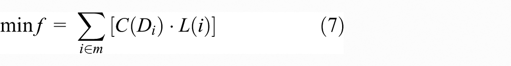
The objective function of diameter optimization of the pipeline network can be expressed as

\min f = \sum_{i \in m} [C (D_{i}) \cdot L (i)]

(7)

and the constraint conditions are as follows

R (i) \cdot D_{i}^{- \frac{16}{3}} \leq P_{i}^{2} - P_{i + 1}^{2} (i = 1, 2, \dots, m)

(8)

P_{\min} \leq P_{i} \leq P_{\max} (i = 1, 2, \dots, m + 1)

(9)

where L(i) is the length of pipe i, m; C(D_i) is the cost function of pipe diameters, and the correlation formula is fitted for cost with the diameter by the least square method. D_i is the diameter of pipe i, cm; R(i) is the flow converting coefficient, R(i) = q(i)²ZΔTL(i)/5033.11², Δ is the relative density; P_i is the pressure at begin point, MPa; P_i + 1 is the endpoint pressure, MPa; P_min is the lowest node pressure constraint, MPa; and P_max is the highest node pressure constraint, MPa.

In the model, equation (8) shows the relationship between the conveying flow of each pipe section and the pressure drop, namely, meeting Weymouth equation, while equation (9) indicates the upper and lower limits of the operating pressure of the pipeline network.

Production system simulation models

The on-site CBM blocks were intensively distributed. The gas production and pipeline operation parameters under construction could be predicted by an integration of the surface/wellbore/surface pipeline networks. When the pipeline networks are integrated, the predicted production data are closer to the actual production data, and can therefore be used to optimize and inform CBM surface construction, and improve CBM production to maximize economic benefit. Several researchers have studied the oil–gas production system, and several models have been proposed. Dempsey et al.¹⁴ were the first to study the coupling of gas reservoir flow simulation and surface system simulation. Startzman et al.,¹⁵ Trick et al.,¹⁶ Litvak and Darlow,¹⁷ Coats et al.,¹⁸ Al-Mutairi et al.,¹⁹ and Güyagüler et al.²⁰ proposed different reservoir/wellbore/surface system integration models. However, all the models were developed for conventional gas reservoirs, and therefore, they cannot be applied to an unconventional gas reservoir like a CBM well because of the adsorbed state and drainage gas recovery mechanism of CBM.

Wellbore model

The CBM wellbore is connected to the surface pipeline network and reservoir. During the CBM production process, the production of CBM is directly determined by the bottomhole flowing pressure (BHFP). Fluid in the annulus could be distinguished by the working fluid level. The gas column is in the upper level, and the aerated fluid column is in the lower level. Several studies have proposed various methods that can be used to calculate BHFP.^9–16

Single-phase flow model

Cullender and Smith²¹ proposed the Cullender–Smith method, which is used to derive the calculation equation for pure gas well bottomhole pressure through an analysis of the energy equation for gas steady flow. The Texas Railroad Commission proposed the average temperature mean deviation coefficient method.²² The equations are as follows

P_{g} = \sqrt{{P_{c}}^{2} e^{2 s} + \frac{1.324 \times 10^{- 18} λ {(TZ q_{sc})}^{2}}{{(d_{2} - d_{1})}^{3} {(d_{2} + d_{1})}^{2}} (e^{2 s} - 1)}

(10)

where

s = \frac{0.03418 γ_{g} H}{TZ}

(11)

Gas-liquid-phase flow model

G Takacs and CG Guffey,²³ J Chen and X Yue,²⁴ RD Oden and JW Jennings,²⁵ Hasan and Kabir,²⁶ Liu et al.,²⁷ and Beggs and Brill²⁸ presented different calculation methods. The Hasan–Kabir²⁶ method is as follows

P_{wf} = P_{c} + Δ P_{g} + r_{L} h_{L} - I_{1} + I_{2}

(12)

I_{1} = \frac{C}{a {(1 - f_{g})}_{avg}} \ln [1 + \frac{a r_{L} {(1 - f_{g})}_{avg} h_{L}}{bC + a (P_{c} + Δ P_{g})}]

(13)

\begin{array}{l} I_{2} = \frac{M_{g} g C h_{L}}{Z R T a} - \frac{M_{g} g C^{2} b}{Z R a^{2} T r_{L} {(1 - f_{g})}_{a v g}} \\ \ln (1 + \frac{a r_{L} {(1 - f_{g})}_{a v g} h_{L}}{b C + a (P_{c} + Δ P_{g})}) \end{array}

(14)

where

C = \frac{q_{sc} TZ p_{sc}}{86, 400 A T_{sc}}

(15)

f_{g} = \frac{v_{sg}}{a + b v_{sg}}

(16)

v_{sg} = \frac{q_{sc} TZ P_{sc}}{A_{a} T_{sc} P}

(17)

Surface pipeline network model

Hydraulic model of pipe

The steady-state hydraulic calculation model for the gas pipeline pressure drop is given as

q = \frac{π}{4} \sqrt{\frac{({P_{Q}}^{2} - {P_{Z}}^{2}) D^{5}}{λ ZRTL}}

(18)

Hydraulic calculation of pipeline network

A pipeline network system consists of n nodes and m sections. The node matrix equation formed by the n continuity equations can be written as equation (19). The relationship between the pressure loss and the section flow rate can be expressed as equation (20). Section pressure drop can be expressed by the pressure difference between the two endpoints of the section (equation (21))

AQ = q

(19)

Q = ϕ (Δ P)

(20)

Δ P = A^{T} P

(21)

When equations (20) and (21) are substituted into equation (19), the following node method mathematical model can be derived

A [ϕ (A^{T} P)] = q

(22)

Thermodynamic calculation of pipeline network

The steady-state thermodynamic calculation is based on the steady-state hydraulic analysis. The Gertjan Zuilhof temperature drop formula is frequently used in gas pipeline temperature drop calculation

T = T_{0} + (T_{Q} - T_{0}) e^{- ax}

(23)

The network node temperature can be calculated by the Wei et al.²⁹ equation

T_{i} = \frac{\sum_{k = 1}^{m} a_{ik} q_{k} c_{k} T_{k}^{R} + q_{gi} c_{gi} T_{gi}}{q_{ii} c_{i}}

(24)

Reservoir model

As three phases coexist in CBM, that is, coal, gas, and water, the method used to predict the productivity of CBM wells is different from that used for conventional gas reservoirs. Thus far, some researchers have tried to predict production performance using the CBM reservoir numerical simulation.³⁰ However, this approach requires a large amount of production and geological data, which make the calculations of the simulation difficult to solve. In this article, a material balance method is utilized to forecast the CBM well production performance simply and effectively.

Langmuir sorption isotherm

CBM is mainly stored as an adsorption state on the coal surface. The Langmuir sorption isotherm equation is usually used to describe the relationship between the adsorption gas volume and pressure

V = \frac{V_{L} P_{r}}{P_{L} + P_{r}}

(25)

Material balance method

The CBM formation reserve equals the sum of the amount of adsorption and free gas

V_{r} = ρ_{b} Ah \frac{V_{L} P_{r}}{P_{L} + P_{r}} + \frac{ϕ Ah (1 - S_{w})}{B_{g}}

(26)

Material balance models include the King model, the Seidle model, and the Jensen–Smith model, of which the King³¹ model is the most commonly used. This model assumes that the gas adsorption and desorption equilibrium follow Langmuir sorption isotherms. Gas productivity can be written in the following form

G_{p} = ρ_{b} Ah V_{L} (\frac{P_{i}}{P_{L} + P_{i}} - \frac{P_{r}}{P_{L} + P_{r}})

(27)

Substituting the formation coefficient into equation (27) generates the following form

G_{p} = ϕ_{i} Ah \frac{T_{sc} Z_{sc}}{P_{sc} T_{r}} (\frac{P_{i}}{Z_{i}^{*}} - \frac{P_{r}}{Z^{*}})

(28)

where

Z^{*} = \frac{Z}{[1 - c_{f} (P_{i} - P_{r})] (1 - {\bar{S}}_{W}) + \frac{ρ_{b} B_{g}}{ϕ_{i}} \frac{V_{L} P_{r}}{P_{L} + P_{r}}}

(29)

{\bar{S}}_{w} = \frac{S_{wi} [1 + c_{w} (P_{i} - P_{r})] + \frac{5.615 (W_{e} - B_{w} W_{P})}{ϕ_{i} Ah}}{[1 - c_{f} (P_{i} - P_{r})]}

(30)

Original gas in place (OGIP) could be calculated as follows

OGIP = ϕ_{i} Ah \frac{T_{sc} Z_{sc} P_{i}}{P_{sc} T_{r} Z_{i}^{*}}

(31)

Substituting equation (31) into equation (28) generates a linear relationship between the average gas reservoir pressure and the cumulative gas production

\frac{P_{r}}{Z^{*}} = - \frac{P_{i}}{Z_{i}^{*} (OGIP)} G_{P} + \frac{P_{i}}{Z_{i}^{*}}

(32)

At the beginning of undersaturated CBM well exploration, formation water is the main product as gas production is so minimal that it can be ignored. Gas production in the well remains constant. The formation pressure difference equation at this time can be written as

P_{r} - P_{wf} = \frac{q_{w} t}{c_{t} N_{w}} + \frac{141.2 B_{w} μ_{w} q_{w}}{kh} (\ln \frac{r_{e}}{r_{wa}} - \frac{3}{4})

(33)

N_{w} = \frac{7758 ϕ Ah}{B_{w}}

(34)

Productivity prediction

The gas production equation for CBM is given as

q_{g} = \frac{k_{g} h [m (P_{r}) - m (P_{wf})]}{1422 T [\ln \frac{r_{e}}{r_{w}} - \frac{3}{4} + s_{f}]}

(35)

where m(P) is the gas pseudo-pressure whose definition is

m (P) = \int_{P_{b}}^{P} \frac{P}{μ_{g} Z} d P

(36)

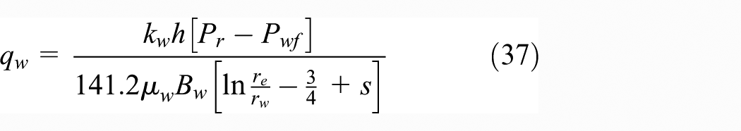
The water production equation for CBM is given as

q_{w} = \frac{k_{w} h [P_{r} - P_{wf}]}{141.2 μ_{w} B_{w} [\ln \frac{r_{e}}{r_{w}} - \frac{3}{4} + s]}

(37)

The relationship between the porosity and permeability is shown below

(\frac{k_{f}}{k_{0}}) = {(\frac{ϕ_{f}}{ϕ_{0}})}^{n}

(38)

The decrease in formation pressure will result in absolute permeability change. This influence can be described using the Palmer–Mansoori³² model

\begin{array}{l} \frac{ϕ}{ϕ_{0}} = 1 + \frac{C_{m}}{ϕ_{0}} (P_{r} - P_{i}) + \frac{ε_{l}}{ϕ_{0}} (\frac{K}{M} - 1) \\ (\frac{P_{r}}{P_{L} + P_{r}} - \frac{P_{i}}{P_{L} + P_{i}}) \end{array}

(39)

C_{m} = \frac{1}{M} - (\frac{K}{M} + f - 1) γ

(40)

\frac{K}{M} = \frac{1}{3} (\frac{1 + ν}{1 - ν})

(41)

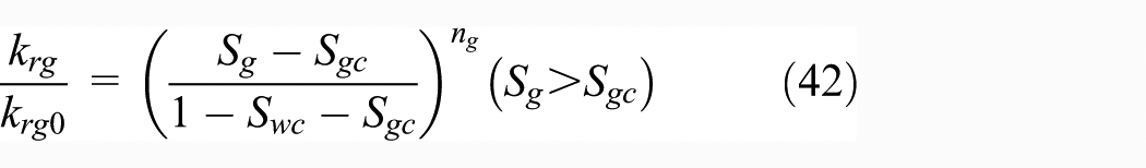
As coal loses its water content, gas and water flowing in the cracks follow Darcy’s Law. When coal saturation changes, the relative gas–water permeability changes as well. To address this issue, Corey³³ presented the equations below

\frac{k_{rg}}{k_{rg 0}} = {(\frac{S_{g} - S_{gc}}{1 - S_{wc} - S_{gc}})}^{n_{g}} (S_{g} > S_{gc})

(42)

\frac{k_{rw}}{k_{rw 0}} = {(\frac{S_{w} - S_{wc}}{1 - S_{wc}})}^{n_{w}} (S_{g} \geq 1 - S_{wc})

(43)

Solution algorithm

The diagram of the CBM surface system optimization design coupled with the productivity prediction is shown in Figure 2. The framework is composed of two main parts: the optimization design and the coupled surface/reservoir simulation. The optimization design is divided into two parts: layout optimization and parameter optimization. The coupled surface/reservoir simulation is made up of three parts: the surface system simulation, the wellbore flow simulation, and the reservoir simulation. The coupling simulation algorithm is shown in Figure 2. The well productivities can be obtained through the production system simulation. During the calculation process, the surface system simulation is used to compute the node pressures and flows of pipeline networks of certain diameters and check the constraint conditions in the process of parameter optimization.

Figure 2.

The diagram of the coalbed methane surface system optimization design coupling the productivity prediction.

Layout optimization algorithm

The layout optimization algorithm of the surface pipeline network is related to the pipeline network form. For example, when the arrangement of the pipeline network follows a tree structure, the goal of optimization is to minimize the total investment in pipelines connecting all the nodes. The optimization problem of the connecting method can be transformed into the minimum spanning tree problem in the undirected graph. At this time, the solving algorithm mainly includes the Kruskal³⁴ algorithm, Prim³⁵ algorithm, and Steiner algorithm.^36–38 The Prim algorithm, which is also called the edge cut method, was proposed by Robert Prim formally in 1957. The specific steps of the Prim algorithm are as follows:

Calculate the weighted distance matrix W_m × m of the graph;

Set up a point set V and select a valve group randomly as the vertex v₁ to add to the set V. Then, set the weight of all the vertices that are not included in V, D(v_i) = W_1i and set up a edge set E to store the edges of the spanning tree, which is currently empty;

In the complement set of V, select the vertex v_j whose weight is minimal to put into V and add the edge k between the vertex v_j and the vertex v_k that makes the weight of v_j minimal to the edge set E;

Modify the weights of all the vertices that are not included in V. If v_l ∉ V, W_kl < D(v_l), and the edge (v_k, v_l) exists, make D(v_l) = W_kl. Otherwise, keep D(v_l).

When all the vertices are included in V, end the calculation; otherwise, return to step (3).

Diameter optimization algorithm

The pipe diameter optimization model is a typical nonlinear optimization problem with constraints. This type of problem is much more complicated than the unconstrained problem, and it is also more difficult to solve. Thus, the problem-solving process is also more diverse. Currently, the widely used methods include the penalty function method, the reduced gradient method, and the Lagrange multiplier method. The penalty function method can also be divided into the external point method, the interior point method, and the mixed penalty function method. The external point method does not impose a high requirement on the initial value, and it is applicable to optimization problems with equality constraints and inequality constraints. Therefore, the external point method is chosen here to solve the pipe diameter optimization problem of the tree pipeline network. The specific iterative steps are as follows:

Construct the penalty function with constraints as follows

α (X) = \sum_{i = 1}^{m} μ [g_{i} (X)] \cdot {[g_{i} (X)]}^{2}

(44)

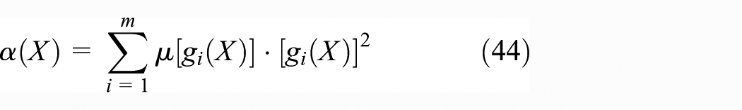
where g_i(X) is the ith constraint condition, m is the total number of constraint conditions, and $μ [g_{i} (X)]$ is the decision variable for 0 and 1. When it satisfies the ith constraint condition, the value of the decision variable is 0. Otherwise, its value is 1.

In the pipe diameter optimization problem, the constraint conditions are as follows

g_{i} (X) = P_{i}^{2} - P_{i + 1}^{2} - R (i) \cdot D_{i}^{- \frac{16}{3}} \leq 0

(45)

g_{i + n} (X) = P_{\min} - P_{i} \leq 0

(46)

g_{i + 2 n} (X) = P_{i} - P_{\max} \leq 0

(47)

The penalty function is

α (X) = \sum_{i = 1}^{3 n} μ [g_{i} (X)] \cdot {[g_{i} (X)]}^{2}

(48)

where X is the solution of the objective function, which contains not only the pipe diameter of each pipe section but also the beginning pressure and the ending pressure.

Add the penalty equation (48) to the original function according to the following equation and construct the augmented objective function

F (X, M_{k}) = f (X) + M_{k} α (X)

(49)

where f(X) is the original objective function and M_k is the penalty factor, M_k + 1 = CM_k, in which C is the amplification factor.

Then, the augmented objective function of the problem is

min F = \sum_{i \in n} [C (D_{i}) \cdot L (i)] + M_{k} \sum_{i = 1}^{3 n} μ [g_{i} (X)] \cdot {[g_{i} (X)]}^{2}

(50)

Select the initial point X₀ and make the initial penalty factor M₁ = 10. Then, set the iterative count k = 1;

Assume that the iterative point X_k_− 1 has been obtained. Then, take X_k_− 1 as the initial point and use the Powell method to solve the unconstrained optimization problem, namely, equation (50). The node pressures are obtained by the pipeline network simulation program, and X_k is set as the extreme value point;

If M_kα(X) ≤ ε (ε is the precision), X_k is the desired optimal solution. End the calculation; otherwise, turn to step (6);

Make M_k + 1 = CM_k, k = k + 1, then return to step (4).

Production system coupling calculation

The CBM production system coupling calculation model integrates the well productivity prediction model, the wellbore calculation model, and the surface pipe network model. The production parameters, such as formation pressure, bottomhole pressure, and gas production, can be determined by coupling iterations of the three models. The diagram describing the CBM production system is shown in Figure 3.

Figure 3.

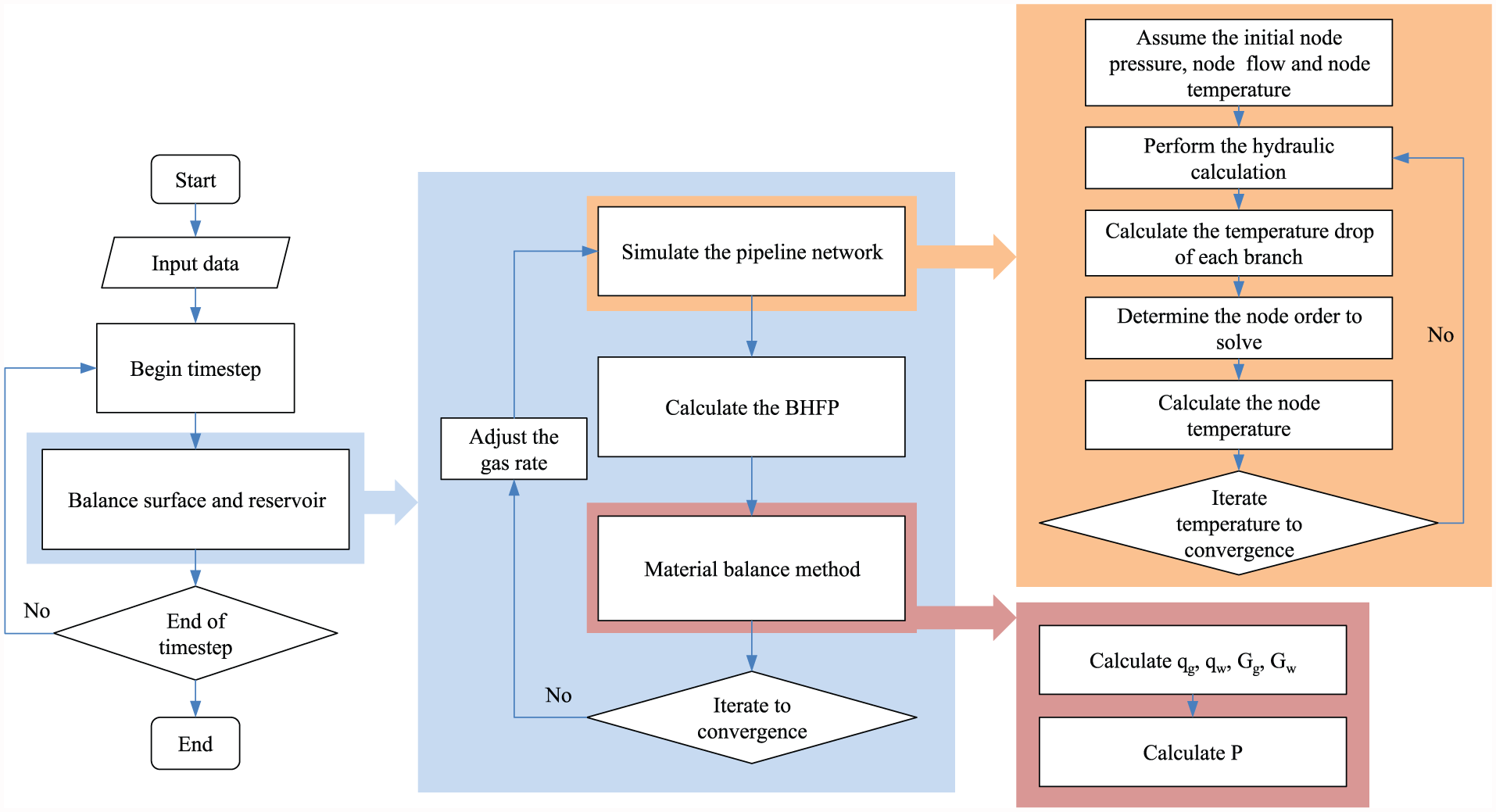
CBM reservoir/surface coupling algorithm.

The specific calculation process is described below:

Input the basic data;

Estimate the initial iteration value of gas production; then, calculate the wellhead pressure based on the surface pipe network model;

According to the wellhead pressure and gas production value, use the wellbore model to calculate the BHFP;

According to the calculated BHFP, use the CBM reservoir productivity prediction model to calculate the gas production at the end of the production period;

Compare the calculated value and the assumed value. If it satisfies the error precision, calculate the cumulative gas production and cumulative water production. If not, replace the calculated value as the initial iteration value; then, repeat steps (3)–(5);

If the end of the production period is reached, the calculation ends. If not, repeat steps (2)–(5).

BHFP calculation algorithm

The calculation process is described below:

The working fluid level pressure P_g is unknown. Estimate an initial value in order to obtain the average pressure and average temperature;

Calculate the gas deviation factor and the friction coefficient at the average pressure and average temperature;

Substitute the results into equations (1) and (2) to calculate P_g;

Compare the calculated result and the estimated value. If the error requirement is not met, the calculated result is used as the estimated value. Then, repeat steps (1)–(3);

Estimate the initial value of P_wf. Calculate the average pressure and average temperature;

Calculate the average deviation coefficient Z;

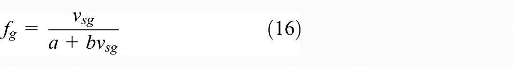
According to equation (8), v_sg is calculated to determine the values of a and b;

After evaluating I₁ and I₂, P_wf is calculated from equation (3);

Compare the calculated result and the estimated value of P_wf, and if it does not meet the error requirement, the calculated result is used as the estimated value. Then, repeat steps (5)–(8).

Surface network parameter calculation

The calculation of the gas phase pipeline network parameters is a coupling hydraulic/thermodynamic iterative process. The specific calculation steps are described below:

Input the basic data of the pipeline network, including pipe length, diameter, absolute roughness, and gas composition;

Estimate the initial values of P ₀, q ₀, and T ₀. The initial value of k is 1;

Equation (22) should be calculated using the node method for steady-state hydraulic pipe network. P_k and q_k under the current node temperature vector T _{k
− 1} are obtained;

Using equation (23), Δ T _k under P _k and q _k for each pipe branch is calculated;

The sequence that will be used to determine the network node temperature should be established;

T _k is solved according to each node temperature calculated from the sequence established in step (5) and equation (24);

If $| T_{k} - T_{k - 1} | < ε$ (ε is the error precision), the calculation is stopped. If not, T _k is treated as a new initial value, and k = k + 1. Then, steps (3)–(7) are repeated.

Reservoir simulation

Coal reservoir production can be roughly predicted using the material balance equation and the CBM gas–water production equation. The specific steps are as follows:

Input basic data, including Langmuir volume, Langmuir pressure, bulk density, initial reservoir pressure, and porosity;

OGIP is calculated by equation (31). The desorption pressure that corresponds with the gas reserves is obtained. This result will be compared with the gas reservoir pressure at this time;

If the gas reservoir pressure is larger than the desorption pressure, it means the coalbed is in an undersaturated state. q_w at this time and the cumulative water production in a period Δ T are calculated by equation (37). Then, the cumulative water production is used to calculate the gas reservoir pressure at the end of the time period. Repeat step (3) until the gas reservoir pressure equals the desorption pressure;

If the gas reservoir pressure equals the desorption pressure (supersaturated state of the coalbed is not considered here), it means the coalbed is in a saturated state. Gas and water are produced from the coalbed, and Q_w is calculated. The gas production, q_g, the cumulative gas production, and the cumulative water production are calculated from equation (35). The reservoir pressure at the end of the time period is calculated. Repeat step (4) until the reservoir pressure equals the shut-in pressure.

Examples

To validate the proposed method, the optimization design of a small CBM block is obtained. There are 11 CBM wells in this block, and their coordinates are shown in Table 1. The composition of CBM is shown in Table 2, and the gas properties are obtained by the Benedict-Webb-Rubin-Starling equation. The CBM parameters are presented in Table 3. First, the surface pipeline network is designed with the traditional optimization method. Then, the optimal form and parameters using the pipeline network layout optimization architecture that are coupled with the production simulation are obtained. Finally, the optimization results are analyzed.

Table 1.

Well coordinates.

Number	x-coordinate (m)	y-coordinate (m)
Well 1	100	800
Well 2	630	268
Well 3	761	110
Well 4	918	262
Well 5	1099	119
Well 6	1400	100
Well 7	1201	273
Well 8	1102	488
Well 9	1064	721
Well 10	873	710
Well 11	851	435

Table 2.

Composition of CBM.

Composition	CH₄	C₂H₆	N₂	CO₂
Mole percent (%)	96.17	0.05	3.71	0.07

CBM: Coalbed methane.

Table 3.

Parameters of coal reservoir.

Input parameters	Value
Initial reservoir pressure (MPa)	5.28
Reservoir temperature (K)	304.15
Initial porosity (%)	4.5
Formation thickness (m)	6.2
Drainage area (m²)	90,000
Bulk density (t/m³)	1.45
Gas content (m³/t)	14.1
Langmuir volume (m³/t)	38.16
Langmuir pressure (MPa)	2.38

Traditional optimization

Single-well productivity prediction

The optimized pipeline network design is commonly obtained by simulating the single-well productivity according to the given coal seam parameters. First, gas reservoir engineers perform the productivity calculation regardless of the surface system structure. Then, they carry out the surface pipeline network design with the given productivities.

Single-well productivity simulation results are shown in Figure 4. The figure shows the variations in gas production, water production, and reservoir pressure during the 10 years after the start of the exploitation. It can be observed that, at the beginning of the production, the reservoir water starts to emerge from the gas well. As the emergence of the reservoir water continues, the reservoir pressure drops rapidly, and the gas productivity is zero. During gas production, the quantity of reservoir water emerging from all the gas wells decreases. With the ongoing drainage, the reservoir pressure drops gradually to the critical desorption pressure of CBM; then, the gas begins to desorb. The gas productivity first increases every year, with a gas production peak of 3395.9 m³/d; then, it decreases every year thereafter.

Figure 4.

The results of single-well productivity simulation.

Surface pipeline network optimization design based on the single-well productivity prediction

The gas productivities of all the wells are calculated by the gas reservoir engineers using the gas reservoir simulation software, and it is assumed that all the wells in the block have the same specific well productivity. Currently, when researchers perform surface pipeline network optimization design, they optimize the surface pipeline network under the condition of the given productivity of each well to minimize the investment cost or operating cost. The result of the surface pipeline network layout design is shown in Figure 5. The red dot stands for the gas well. The red hollow square represents the treatment plant. The gas from each well will flow into the treatment plant.

Figure 5.

Layout of the pipeline network based on the single-well productivity prediction.

The proposed optimization method

The surface pipeline network layout obtained when the optimization design architecture described in this article is used is illustrated in Figure 6. The gas flows into the central treatment plant through a separated pipeline. This structure is called a star structure.

Figure 6.

Layout of the star structure pipeline network.

The pipeline network optimization design consists of the layout optimization design and parameter optimization design. The goal of the layout optimization design is to optimize the site locations and connection relationships between nodes. The outcome of the layout optimization design in the example is the star structure that is illustrated in Figure 6.

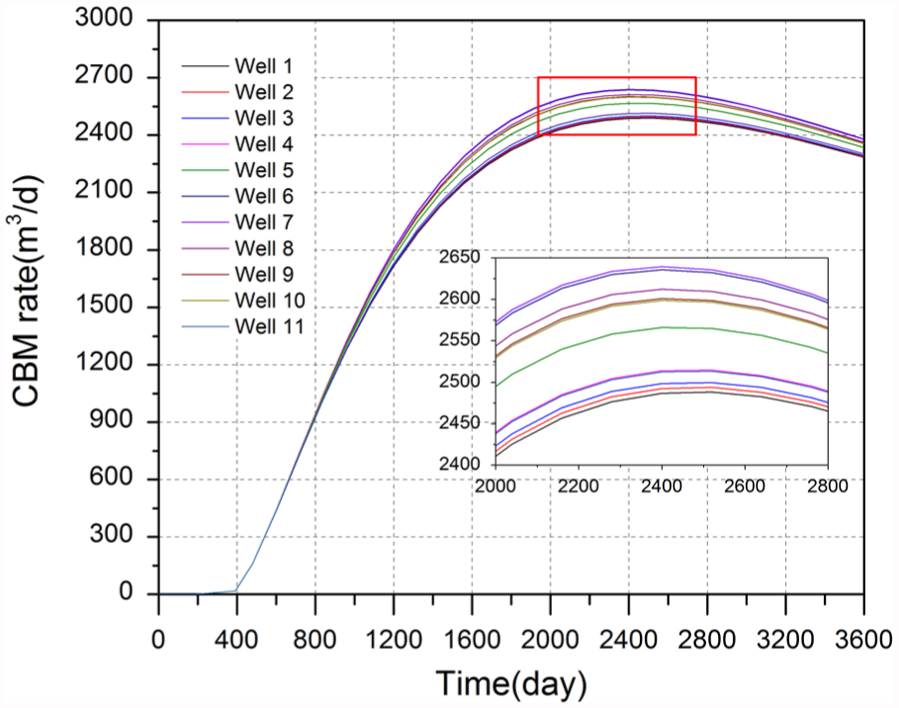
The gas productivity of each well under this pipeline network structure is shown in Figure 7. The gas productivity trend of each gas well is almost the same. All the wells reach the peak gas productivity at the same time, which is about 2800 m³/d. This value is lower than that of the single-well productivity prediction. This is because the surface, the wellbore, and the reservoir are mutually constrained in the coupling calculation of the production system, like the inlet pressure limit of the treatment plant. This causes the gas productivity of the block to be lower than the productivity prediction result of the single reservoir simulation. In the figure, it can be observed that each peak well productivity is slightly different (the red square in the figure).

Figure 7.

Daily gas well production under the star structure.

Analysis of optimization results

Tree surface system

Three types of pipeline network structures can be chosen for a CBM block: the star structure, tree structure, and concatenated structure. Figure 8 shows the gas productivity results when the tree structure obtained by the traditional optimization is adopted and the coupling prediction method of the production system is applied. It can be seen that the gas productivity trends of all the wells change similarly with the time, but their peaks and the times at which the peaks occur are different. The gas productivities of wells No. 1, No. 2, No. 3, and No. 4 reach their peak on the 2520th day, while the gas productivities of wells No. 5–No. 11 reach their peak on the 2400th day. In addition, the gas productivity of well No. 7, which is closest to the treatment plant, is maximal, while the gas productivity of well No. 1, which is farthest from the treatment plant, is minimal. This observation may be explained as follows. As the distance of a well from a treatment plant increases, the pipeline pressure drop also increases, which increases the wellhead back pressure. This affects the BHFP, causing a deterioration in gas productivity. Figures 4 and 8 show that, for the surface pipeline network optimization design based on the single-well productivity prediction, the assumption that all the gas well productivities are the same is inconsistent with the actual situation. This optimization design method cannot accurately reflect actual production. Furthermore, the optimization results it generates are unreasonable, making the structure unfavorable and decreasing profits.

Figure 8.

Daily gas well production under the tree structure.

Concatenated surface system

The surface system is a part of the CBM production system; therefore, its pipeline network structure has an influence on gas production. Besides a star structure and a tree structure, the CBM surface system can also adopt a concatenated structure, which is shown in Figure 9. The productivity prediction result of each gas well when the concatenated structure is adopted is shown in Figure 10. It can be seen that the gas productivity trend is similar to those obtained when the star structure and the tree structure are adopted.

Figure 9.

Layout of the concatenated structure pipeline network.

Figure 10.

Daily gas well production under the concatenated structure.

Influence of different surface structures on the production

The analysis of the results of the single-well productivity prediction and calculations of the star structure, tree structure, and concatenated structure coupling the productivity are shown in Figure 11. It can be seen from the figure that the gas productivity peak of the single-well productivity prediction is maximal, while the peaks of the star structure, concatenated structure, and the tree structure reduce in turn. Affected by the surface system structure, the well productivities of different structures vary. Taking well No. 1 as an example, the gas productivity of the star structure is maximal, while the gas productivity of the concatenated structure takes second place, and the gas productivity of the tree structure is minimal. In terms of the cumulative production (Figure 12), the star structure achieves a maximal value, while the concatenated structure takes second place, and the tree structure achieves a minimal value.

Figure 11.

Contrast diagram of single-well productivity under different pipeline network forms.

Figure 12.

Cumulative gas productivities of a block under different pipeline network forms.

Influence of optimization goal on the optimization result

The goal of the traditional optimization method is to minimize investment. It can be seen from Figure 13(a) that the pipeline network investment when the tree structure is adopted is lower than those when the concatenated structure and the star structure are adopted, with the concatenated structure offering greater savings than the star structure. In this article, the goal of the optimization is to maximize system profits, which conforms more to the requirements of gas field operation. Figure 13(c) shows that the profit of the star structure is maximal, while that of the tree structure is minimal, increasing the profit by about 2 million dollars compared with that of the traditional optimization method. The profit achieved when the concatenated pipeline network is applied falls in between the maximal and minimal values. Figure 13(b) shows that the star structure improved gas productivity by 10.9% compared with the tree structure.

Figure 13.

The contrast diagram of (a) investment, (b) gas productivity, and (c) profit under different pipeline network forms.

Summary

A surface system layout optimization architecture coupled with a simulation of the production system is proposed. Unlike the traditional method, the proposed method does not focus only on the surface system; furthermore, it does not consider the construction investment as the objective function. In this study, the profit in the production cycle is the goal of the design optimization, which is much closer to the actual situation. The surface system simulation adopts the node method and couples the thermal calculation with the hydraulic calculation. The BHFP of the CBM wellbore is computed by combining the Hasan–Kabir analytic method and the average temperature and average deviation coefficient method. The prediction of the coalbed reservoir productivity is based on the material balance method. The case studies showed that the traditional optimization results suggest the tree structure arrangement for the CBM surface pipeline network, while the proposed method recommends the star structure, improving the gas productivity by 10.9% and increasing the profit by 2 million dollars. The proposed method also indicates that the surface pipeline form has a significant influence on the CBM reservoir, which is characterized by low pressure and gas productivity. Although the star structure requires higher investments than the tree structure, the star structure can provide greater profit because it remarkably increases gas productivity. As the CBM reservoir has low gas productivity, the influence of the surface pipeline network information on gas productivity should not be ignored. The method is provided as a reference for CBM surface engineering designs. Currently, most of the CBM blocks in China have adopted the star pipeline network structure.

Footnotes

Appendix 1

Academic Editor: Pietro Scandura

Declaration of conflicting interests

The author(s) declared no potential conflicts of interest with respect to the research, authorship, and/or publication of this article.

Funding

The author(s) disclosed receipt of the following financial support for the research, authorship, and/or publication of this article: This work was financially supported by the Young Scholars Development Fund of SWPU (201599010096).

References

Yang

. Brief discussion on development of coal seam gas industry in China. SCI-TECH Innov Prod 2011; 8: 20–22.

Dijkstra

. A note on two problems in connexion with graphs. Numer Math 1959; 1: 269–271.

Coats

. Optimum location of trunk lines in oil and gas fields. J Petrol Tech 1963; 15: 1019–1024.

Rothfarb

Frank

Rosenbaum

. Optimal design of offshore natural gas pipeline systems. Oper Res 1970; 18: 992–1020.

Shamir

. Optimal route for pipelines in two-phase flow. Soc Petrol Eng J 1971; 9: 215–222.

Bhaskaran

Salzborn

. Optimal diameter assignment for gas pipeline networks. J Australia Math Soc 1979; 21: 129–144.

Simpson

Dandy

Laurey

. Genetic algorithm compared to other techniques for pipe optimization. Water Resource Plan Manage 1994; 120: 423–443.

Boyd

Surry

Radcliffe

. Constrained gas network pipe sizing with genetic algorithm. Technical report EPCC-TR94-11, November, 1994. Edinburgh: Edinburgh Parallel Computing Center.

Hansen

Madsen

Nilsen

. Optimization of pipe networks. Math Program 1991; 52: 45–58.

10.

Wolf

Smeers

. Optimal dimensioning of pipe networks with application to gas transmission networks. Oper Res 1996; 44: 596–608.

11.

Zhang

Zhu

. A bilevel programming method for pipe network optimization. J Optim 1996; 6: 838–857.

12.

El-Mahdy

OFM

Ahmed

MEH

Metwalli

. Computer aided optimization of natural gas pipe networks using genetic algorithm. Appl Soft Comput 2010; 10: 1141–1150.

13.

Stoner Associates, Inc. Technical data book SynerGEE gas, version 3.2. Houston, TX: Stoner Associates, Inc., 2000.

14.

Dempsey

Patterson

Coats

. An efficient model for evaluating gas field gathering system design. J Petrol Tech 1971; 23: 1067–1073.

15.

Startzman

Brummet

Ranney

. Computer combines offshore facilities and reservoir forecasts. Petrol Eng 1977; 49: 65–74.

16.

Trick

Agarwal

Ammer

. Gas-field deliverability forecasting: a coupled reservoir simulator and surface facilities model. Morgantown, WV: USDOE Morgantown Energy Technology Center, 1994.

17.

Litvak

Darlow

. Surface network and well tubinghead pressure constraints in compositional simulation. In: Proceedings of the SPE reservoir simulation symposium, San Antonio, TX, 12–15 February 1995. Richardson, TX: Society of Petroleum Engineers.

18.

Coats

Fleming

Watts

. A generalized wellbore and surface facility model, fully coupled to a reservoir simulator. SPE Reservoir Eval Eng 2004; 7: 132–142.

19.

Al-Mutairi

Hayder

Al-Shammari

. A study of coupling surface network to reservoir simulation model in a large Middle East field. In: Proceedings of the North Africa technical conference and exhibition, Cairo, Egypt, 14–17 February 2010. Richardson, TX: Society of Petroleum Engineers.

20.

Güyagüler

Zapata

Holmes

. Near-well-subdomain simulations for accurate inflow-performance-relationship calculation to improve stability of reservoir/network coupling. SPE Reservoir Eval Eng 2011; 14: 634–643.

21.

Cullender

Smith

. Practical solution of gas-flow equations for wells and pipelines with large temperature gradients. Richardson, TX: Society of Petroleum Engineers, 1956, pp.281–287.

22.

Yang

. Gas extraction engineering. Beijing, China: Petroleum Industry Press, 2001, pp.47–50.

23.

Takacs

Guffey

. Prediction of flowing bottomhole pressures in gas wells. In: Proceedings of the SPE gas technology symposium, Dallas, TX, 7–9 June 1989, SPE-19107-MS. Richardson, TX: Society of Petroleum Engineers.

24.

Chen

Yue

. Pressure gradient of gas liquid mixture in pumping well. J Daqing Petrol Inst 1985; 4: 31–39.

25.

Oden

Jennings

. Modification of the Cullender and Smith equation for more accurate bottomhole pressure calculations in gas wells. In: Proceedings of the Permian basin oil and gas recovery conference, Midland, TX, 10–11 March 1988, p.10. Richardson, TX: Society of Petroleum Engineers.

26.

Hasan

Kabir

. A study of multiphase flow behavior in vertical wells. SPE Prod Eng 1988; 3: 263–272.

27.

Liu

. Prediction of flowing bottomhole pressures for two-phase coalbed methane well. Acta Petrol Sin 2010; 31: 998–1003.

28.

Beggs

Brill

. A study of two-phase flow in inclined pipes. J Petrol Tech 1973; 5: 601–617.

29.

Wei

Liu

Ren

. Node parameter calculation method of oil and gas gathering pipeline network. J Daqing Petrol Inst 2003; 27: 79–83.

30.

Thomas

Dale

. The use of numerical simulation in predicting coalbed methane producibility from the Gates coals, Alberta Inner Foothills, Canada: comparison with Mannville coal CBM production in the Alberta Syncline. Int J Coal Geo 2008; 74: 215–236.

31.

King

. Material balance techniques for coal seam and Devonian shale gas reservoirs. In: Proceedings of the SPE annual technical conference and exhibition, New Orleans, LA, 23–26 September 1990, pp.181–192. Richardson, TX: Society of Petroleum Engineers.

32.

Palmer

Mansoori

. How permeability depends on stress and pore pressure in coalbeds: a new model. In: Proceedings of the SPE annual technical conference and exhibition, Denver, CO, 6–9 October 1996, pp.557–565. Richardson, TX: Society of Petroleum Engineers.

33.

Corey

. Effect of stratification on relative permeability. J Petrol Tech 1956; 8: 69–71.

34.

Kruskal

. On the shortest spanning subtree of a graph and the traveling salesman problem. Proc Am Math Soc 1956; 7: 48–50.

35.

Prim

. Shortest connection networks and some generalizations. Bell Syst Tech J 1957; 36: 1389–1401.

36.

Chang

. The generation of minimal trees with a Steiner topology. J Assoc Comput Mach 1972; 19: 699–711.

37.

Gibert

Pollak

. Steiner minimal trees. SIAM J Appl Math 1968; 16: 1–29.

38.

Hanan

. On Steiner’s problem with rectilinear distance. SIAM J Appl Math 1966; 14: 255–265.

Optimization design of coalbed methane pipeline network–coupled wellbore/reservoir simulation

Abstract

Keywords

Introduction

Mathematical model of optimization

Layout optimization

Diameter optimization

Production system simulation models

Wellbore model

Single-phase flow model

Gas-liquid-phase flow model

Surface pipeline network model

Hydraulic model of pipe

Hydraulic calculation of pipeline network

Thermodynamic calculation of pipeline network

Reservoir model

Langmuir sorption isotherm

Material balance method

Productivity prediction

Solution algorithm

Layout optimization algorithm

Diameter optimization algorithm

Production system coupling calculation

BHFP calculation algorithm

Surface network parameter calculation

Reservoir simulation

Examples

Traditional optimization

Single-well productivity prediction

Surface pipeline network optimization design based on the single-well productivity prediction

The proposed optimization method

Analysis of optimization results

Tree surface system

Concatenated surface system

Influence of different surface structures on the production

Influence of optimization goal on the optimization result

Summary

Footnotes

Appendix 1

Declaration of conflicting interests

Funding

References