Friction coefficient in mixed lubrication: A simplified analytical approach for highly loaded non-conformal contacts

Abstract

This article presents an analytical model for predicting friction in mixed lubrication regime. The calculations consider load shared between roughness asperities and the lubricant film, as well as the appearance of thermal effects in the contact and the influence of the lubricant rheology. Tests using tribometers have been performed to measure the friction coefficient in non-conformal surfaces for both point and line contacts. This allows verifying the results of the model under a broad range of experimental conditions with an influence on the lubrication conditions. Reasonably good precision has been found in the results obtained, which combined with a simplicity of use confers the model a high practical utility for rough estimates of the friction coefficient under mixed lubrication.

Introduction

The increasing development of tribological studies has improved our knowledge of the mechanisms of lubrication that take place in highly loaded non-conformal contacts,^1–3 such as those that occur in gears, rolling contact bearings, cams and tappets.

These contacts can operate in elastohydrodynamic lubrication when there is a complete separation of surfaces, resulting in fluid film lubrication.^4,5 However, demanding working conditions often cause a loss in continuity of the lubrication film and the existence of direct contacts between surface asperities. ⁶

Mixed lubrication takes place in these conditions and the physical-chemical interactions between the surfaces lead to an increase in the friction coefficient. ⁷ As this effect becomes increasingly pronounced, it tends towards a boundary lubrication regime, which is characterised by the roughness asperities withstanding the entire load.^3,6

As a result of an intensive research, numerous models^7–11 have been developed to predict friction (or traction) coefficient and other parameters of interest in non-conformal contacts under mixed lubrication, with increasing levels of precision and complexity, especially through the use of simulations based on numerical calculations.

Simultaneously, other more simplified models have been proposed,^12,13 the utility of which is based on the possibility of obtaining reasonably good estimates in a faster and simpler way, which is the objective of the analytical model proposed herein.

Olver and Spikes ¹⁴ have developed a simple method to calculate friction coefficient in elastohydrodynamic lubrication, which is based upon viscoelastic Maxwell-Eyring rheology. Later studies of Morales-Espejel and Wemekamp ¹⁵ have proposed other simplified solutions for Newtonian, Eyring and limiting shear stress fluids in full film lubrication. These models^14,15 take thermal effects into account and allow sufficiently accurate predictions to be obtained by means of simple iterative calculations, providing the user with physical understanding of the phenomena involved. Friction calculations in mixed lubrication frequently combine models for boundary lubrication and fluid-film conditions. Morales-Espejel et al. ¹⁶ and Popovici and Schipper ¹⁷ have published approaches for deterministic microcontact models and Eyring fluids.

The so-called Eyring fluids use a hyperbolic sine law that has shown to be less suitable than other models to replicate the experimental behaviour of shear-thinning lubricants.^18–20 In this article, the Carreau equation is considered, bearing in mind that Jang et al., ²⁰ Chapkov et al. ²¹ and Liu et al. ²² have reported an extensive set of numerical solutions and comparisons with experiments, which reveal that the Carreau model properly characterises the shear-thinning effects, in particular for the case of the mineral base and the polyalphaolefin lubricants^23–25 used in this work.

Concerning the mixed lubrication analysis, unlike models based on the detailed geometry of the asperities^16,17 which generally complicate the use of analytical or semi-analytical algorithms, we use a macroscopical approach that only requires the use of a standardised statistical roughness parameter. In this way, we aim for an approach even more simplified than the aforementioned models, in order to develop a fully analytical model.

This article completes a series of works from the authors to predict friction in non-conformal contacts through analytical methods. Lafont et al. ¹³ present the isothermal elastohydrodynamic calculation for point contact, which is generalised in Echávarri et al. ²⁵ under thermal effects. Based on the latter methodology, Echávarri et al. ²⁶ present the development of the model for thermal-elastohydrodynamic line contact.

We hereby present a procedure for analytical evaluation under mixed lubrication conditions, including the calculation equations for point and line non-conformal contacts, which considers operating conditions: load, temperature, average velocity and sliding velocity. It also takes the lubricant rheology into account, modelling piezoviscous, pseudoplastic behaviours as well as local thermal effects, and the thermal and elastic properties of the contacting bodies, their geometry and surface finish.

Mixed film lubrication model

The Stribeck curve ⁵ displayed in Figure 1 represents the trend of the friction coefficient depending on the value of the specific lubricant film thickness λ. This value is defined in equation (1) from the minimum lubricant film thickness h₀ and the root mean square (RMS) roughness of the two surfaces in contact σ₁, σ₂

$$\lambda =\frac{h_0}{\sqrt{{\sigma }_1^2+{\sigma }_2^2}}$$

(1)

Figure 1.

Stribeck curve illustrating lubrication regimes of non-conformal contacts.

The elastohydrodynamic lubrication regime corresponds to λ values greater than 2; for lower values, the lubricant film ceases to be continuous and the contact operates under mixed lubrication,^6,27 so that part of the load is supported through pressurised lubricant and the other part through direct contact between surface asperities.

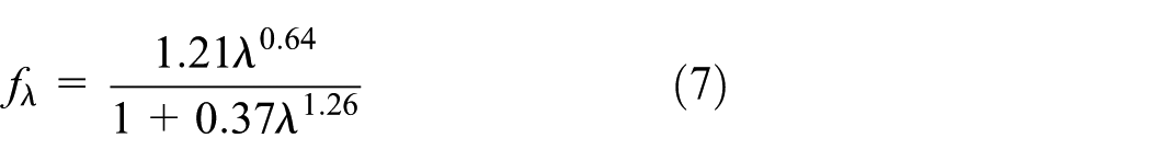
Depending on the specific film thickness, an estimate can be established of the normal load supported by the lubricant film W_L and that supported by the roughness asperities in boundary lubrication W_B. If the load share function f_λ is defined as the quotient between the load supported by the lubricant film and the total load W_T, the result is equation (2)

$$W_L=f_{\lambda }{W}_T$$

(2)

So that the load supported by the roughness asperities results

$$W_B=(1-f_{\lambda })W_T$$

(3)

As per Castro and Seabra, ⁷ both film thickness and load share function can be considered as constant along the contact. Therefore, the pressure distribution in mixed film regime p is the result of the expression (4), based on the existing pressures in rough elastohydrodynamic lubrication p_ER and boundary lubrication p_B, calculated with the loads W_L and W_B, respectively

$$p=p_{\mathrm{ER}}+p_B$$

(4)

Furthermore, considering the deduction process followed by Castro and Seabra, ⁷ equation (5) is attained for the friction force F_T. It takes into account equations (2) and (3), together with the results of Winter and Michaelis ²⁸ to relate the friction coefficients in rough elastohydrodynamic conditions µ_ER and full film lubrication µ_E. The ensuing friction coefficient under mixed lubrication µ is given by equation (6)

$$F_T={\mu }_{\mathrm{ER}}{W}_L+{\mu }_B{W}_B\approx {\mu }_E{f}_{\lambda }^{1.2}{W}_T+{\mu }_B(1-f_{\lambda })W_T$$

(5)

$$\mu =\frac{F_T}{W_T}=f_{\lambda }^{1.2}{\mu }_E+(1-f_{\lambda }){\mu }_B$$

(6)

where the friction coefficients in full film lubrication µ_E and boundary lubrication µ_B are calculated with the loads W_L and W_B, respectively.

Therefore, calculating friction in mixed lubrication for highly loaded non-conformal contacts requires a load share function and the friction coefficients in both elastohydrodynamic and boundary conditions.

In order to determine the fraction of load supported by the lubricant film, Zhu and Hu ¹¹ propose the load share function (7) for point contact

$$f_{\lambda }=\frac{1.21{\lambda }^{0.64}}{1+0.37{\lambda }^{1.26}}$$

(7)

Similarly, for line contacts, Castro and Seabra ⁷ suggest the expression (8)

$$f_{\lambda }=0.84{\lambda }^{0.23}$$

(8)

Figure 2 compares both functions, which although present certain variations in some sections, do not differ significantly.

Figure 2.

Comparison of load share functions.

With regard to the friction coefficient, various results have been published for boundary lubrication.^4,29,30 In the case of steel–steel contacts, values have been determined around 0.07–0.15, which depend on the type and amplitude of the roughness, ¹¹ with higher values corresponding to polished surfaces. Their value can be determined experimentally, ¹⁷ for example, through a prior characterisation test in a tribometer with specific film thickness tending to zero, so that the elastohydrodynamic contribution is negligible. The determination of the friction coefficient in elastohydrodynamics is discussed in the following section.

Friction coefficient in fluid film lubrication

In elastohydrodynamic lubrication regime, the viscous properties of the fluid play a fundamental role on friction. The Carreau ³¹ model is one of the most used in the literature ³² to determine generalised viscosity η_G for pseudoplastic (or shear-thinning) lubricants under severe operating conditions typical of elastohydrodynamics.

In the Carreau equation (9), the piezoviscous behaviour of the lubricant is represented using Barus’ law and shear rate $\stackrel{·}{\gamma }$ is simplified to the Couette component, ²⁶ as customary for analyses of traction

$$\begin{array}{c}{\eta }_G=\eta {[1+{\left(\frac{\eta \stackrel{·}{\gamma }}{G}\right)}^2]}^{\frac{n-1}{2}};\mathrm{with}\eta ={\eta }_0{e}^{\alpha p_E},\hfill \\ \alpha ={\left[\underset{0}{\overset{\infty }{\int }}\frac{\eta (p=0)\mathrm{dp}}{\eta (p)}\right]}^{-1},\mathrm{and}\stackrel{·}{\gamma }=\frac{\Delta u}{h}\hfill \end{array}$$

(9)

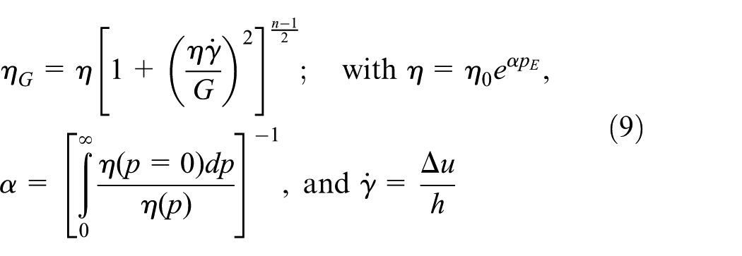
where η₀ is the viscosity at ambient pressure, α the reciprocal asymptotic isoviscous pressure coefficient, p_E the elastohydrodynamic pressure, G the shear modulus, n the power-law exponent, Δu the sliding velocity and h the film thickness.

In these conditions, it is possible to calculate the shear stress distribution ${\tau }_E$ , whose integration in the contact area A allows calculating the force of friction, and dividing by normal load we find the friction coefficient

$${\tau }_E={\eta }_G\stackrel{·}{\gamma }$$

(10)

In order to integrate in an analytical way, two simplifying hypotheses are considered that have proven to be reasonable in prior elastohydrodynamic lubrication studies: ²⁴ a pressure based on Hertzian distribution and a constant film thickness. ³ The results of the integration are expressed as a function of the effective pressure p_ef ³³

$${\mu }_E=\frac{A}{W_L}{\left(\frac{{\eta }_0\Delta u}{h}\right)}^n{G}^{1-n}{e}^{n\alpha p_{\mathrm{ef}}}$$

(11)

Muraki and Dong ³³ provide the result of effective pressure for a case of Newtonian point contact and the same methodology can be used for a generalisation using the Carreau model. The result is shown in equation (12) for point contact, which corresponds to the Newtonian case when n = 1. Likewise, the effective pressure result can be determined for the Carreau model in a line contact, presented in equation (13). The results obtained are in accordance with the friction coefficient expressions proposed in Lafont et al. ¹³ and Echávarri et al. ²⁶

$$p_{\mathrm{ef}}=\frac{1}{n\alpha }\ln [\frac{2e^{n\alpha p_0}}{n\alpha p_0}(1-\frac{1}{n\alpha p_0})+\frac{2}{{\left(n\alpha p_0\right)}^2}]$$

(12)

$$p_{\mathrm{ef}}=\frac{1}{n\alpha }\ln [1+\frac{\pi n\alpha p_0}{12}(\frac{2+\sqrt{3}}{2}{e}^{n\alpha p_0\sqrt{\frac{1}{2}-\frac{\sqrt{3}}{4}}}+e^{n\alpha p_0\frac{\sqrt{2}}{2}}+\frac{2-\sqrt{3}}{2}{e}^{n\alpha p_0\sqrt{\frac{1}{2}+\frac{\sqrt{3}}{4}}})]$$

(13)

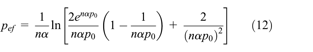
where p₀ is the Hertz (maximum) pressure. For the elastohydrodynamic analysis, p₀ is calculated for the load W_L supported by the lubricant film.

It is worth noting that it is generally accepted that the lubricated conjunction may be separated into zones that operate somewhat independently.^24,34 The film thickness is mainly dependent on the fluid dynamics of the inlet zone, whereas the friction coefficient is essentially determined by the high-pressure rheological behaviour of the lubricant within the high-pressure contact zone.

Film thickness and temperature

The film thickness depends primarily on the inlet conditions in the contact and can be approximated as the central value h_c,^3,34 which can be estimated using equation (14). This expression considers the correction factors due to viscous shear heating effects in the inlet zone ⁴ and those due to the influence of shear-thinning, ²³ assuming they affect point and line contacts in the same way ²⁴

$$\begin{array}{c}{h}_c=h_{\mathrm{Nct}}{[1+0.79{\left((1+\frac{\mathrm{SRR}}{100})\frac{u_m{\eta }_0}{h_{\mathrm{Nct}}G}\right)}^{\frac{1}{1+0.002\mathrm{SRR}}}]}^{-3.6{(1-n)}^{1.7}};\hfill \\ \mathrm{with}{h}_{\mathrm{Nct}}={\phi }_t{h}_{\mathrm{Ncb}}\mathrm{and}\mathrm{SRR}=\frac{\Delta u}{u_m}100\hfill \end{array}$$

(14)

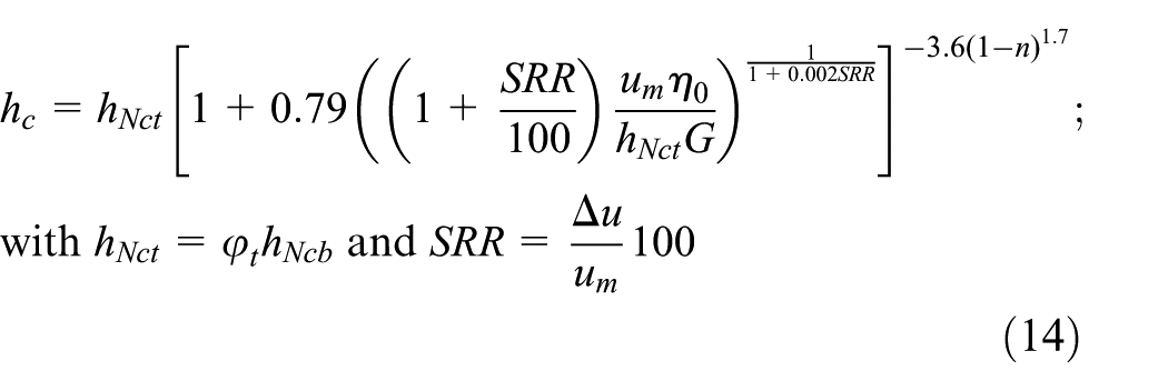
where SRR is the slide-to-roll ratio expressed in percentage, u_m the average velocity and h_Nct the Newtonian central film thickness at inlet temperature. Unlike bath temperature, inlet temperature is initially unknown and the use of a thermal factor ${\phi }_t$ is therefore needed to consider the shear heating effects in the inlet zone, which is calculated with equation (15). The Newtonian central film thickness at bath temperature, h_Ncb, can be calculated using the formulae in Table 1, developed by Hamrock and Dowson for point contact and by Hamrock for line contact.^4,24 This table also provides the formulae for the Hertz (maximum) pressure p₀ and the contact area A for a given normal load W, together with the contact dimension a, that is, contact radius for point contact, half-width of the rectangle for line contact ²

$$\begin{array}{c}{\phi }_t=\frac{1-13.2(p_0/E\prime )L_t^{0.42}}{1+0.213[1+2.23{\left(\frac{\Delta u}{u_m}\right)}^{0.83}]L_t^{0.64}};\hfill \\ \mathrm{with}{L}_t=\frac{\beta {\eta }_0{u}_m^2}{K_l}\hfill \end{array}$$

(15)

Table 1.

Formulae for point and line contacts.

Type of contact	Newtonian compressible central film thickness, hNc	Hertzian results for p0 and a
Point contact $A=\pi a^2$	$1.55{\alpha }^{0.53}{\left({\eta }_0{u}_m\right)}^{0.67}E{\prime }^{0.061}{R}^{0.33}{p}_0^{-0.201}$	$p_0=\frac{3W}{2\pi a^2}$	$a=\sqrt[3]{\frac{3\mathrm{WR}}{2E\prime }}$
Line contact $A=2\mathrm{aL}$	$2.154{\alpha }^{0.47}{\left({\eta }_0{u}_m\right)}^{0.692}E{\prime }^{0.110}{R}^{0.308}{p}_0^{-0.332}$	$p_0=\frac{2(W/L)}{\pi a}$	$a=\sqrt{\frac{8(W/L)R}{\pi E\prime }}$

R is the reduced radius of curvature.

where β is the temperature-viscosity coefficient, K_l the lubricant thermal conductivity and E′ the reduced Young’s modulus.

The viscous properties of the lubricant in friction calculations are assessed at contact temperature T, that is, the average temperature of the lubricant within the high-pressure contact zone. This temperature is calculated using the classic flash theory of Blok, ³⁵ Jaeger ³⁶ and Archard ³⁷ for dry contact, generalised by Olver and Spikes ¹⁴ for lubricated contacts, and that for low film thickness typical of mixed lubrication can be simplified to equation (16)

$$T=T_{\mathrm{in}}+T_f$$

(16)

The inlet temperature T_in may be calculated from the bath temperature T_b with the formulae in Table 1, equalling the Newtonian central film thickness at T_in, h_Nct = h_Nc(T_in), to the thermal factor in the expression (15) computed at T_b, and multiplied by the Newtonian central film thickness at T_b, h_Nct = φ_t(T_b)·h_Nc(T_b). Equation (17) is attained in the case of point contact and equation (18) in the case of line contact

$$[\alpha (T_{\mathrm{in}}){]}^{0.53}·[{\eta }_0(T_{\mathrm{in}}){]}^{0.67}={\phi }_t(T_b)·[\alpha (T_b){]}^{0.53}·[{\eta }_0(T_b){]}^{0.67}$$

(17)

$$[\alpha (T_{\mathrm{in}}){]}^{0.47}·[{\eta }_0(T_{\mathrm{in}}){]}^{0.692}={\phi }_t(T_b)·[\alpha (T_b){]}^{0.47}·[{\eta }_0(T_b){]}^{0.692}$$

(18)

The flash temperature rise T_f can be estimated based on the results of the average flash temperature for each surface T_fi, (i = 1,2), which are separately calculated as if all the heat generated was conducted to the body i²

$$\frac{1}{T_f}=\frac{1}{T_{f1}}+\frac{1}{T_{f2}}$$

(19)

Table 2 presents the expressions to determine the average flash temperature of each surface according to Stachowiak and Batchelor. ² The equations to use depend on the Peclet number P_ei, which is related to heat transferred into the bulk of each contacting body i

$$P_{\mathrm{ei}}=\frac{u_{i}a}{2{\chi }_i};\mathrm{where}{\chi }_i=\frac{K_i}{{\rho }_i{\sigma }_i}$$

(20)

Table 2.

Average flash temperatures for point and line contacts. ²

Peclet number	Heat penetration	Type of contact	Average flash temperature, Tfi
Pei < 0.1	High	Point	$0.250\frac{\mu W\Delta u}{K_{i}a}$
		Line	$0.318\frac{\mu (W/L)\Delta u}{K_i{P}_{\mathrm{ei}}}(-2.303P_{\mathrm{ei}}{\log }_{10}2P_{\mathrm{ei}}+1.616P_{\mathrm{ei}})$
0.1 < Pei < 5	Medium	Point	$(0.215-0.0255P_{\mathrm{ei}})\frac{\mu W\Delta u}{K_{i}a}$
		Line	$0.159\frac{\mu (W/L)\Delta u}{K_i{P}_{\mathrm{ei}}}(0.423+2.663·P_{\mathrm{ei}}-0.649·P_{\mathrm{ei}}^2+0.062·P_{\mathrm{ei}}^3)$
Pei > 5	Low	Point	$0.218\frac{\mu W\Delta u}{K_i{\mathrm{aP}}_{\mathrm{ei}}^{1/2}}$
		Line	$0.376\frac{\mu (W/L)\Delta u}{K_i{P}_{\mathrm{ei}}^{1/2}}$

where χ_i represents the thermal diffusivity, K_i the thermal conductivity, ρ_i the density, σ_i the specific heat and u_i the velocity of the surface.

Methodology

An experimental stage has been developed using MTM and MPR commercial testing equipments from PCS Instruments (www.pcs-instruments.com), shown in Figure 3. Both devices can measure the friction coefficient under controlled conditions of temperature, load, average velocity and sliding velocity. The MTM presents a ball and disc contact with a ball radius of 9.525 mm, while the MPR tests line contacts between three identical rings and a central roller with contact diameters of 54 and 12 mm, respectively. The rings present a constant width of 8 mm, whereas the roller geometry is more complex, as depicted in Figure 3. The roller has a contact width of 1 mm, with symmetrical chamfers on both sides to avoid stress peaks on the edges. The experimental setup allows an evenly distributed normal load along the three contacts among the rings and the roller in the MPR.

Figure 3.

Overview of the MTM and the MPR. Detail of the roller.

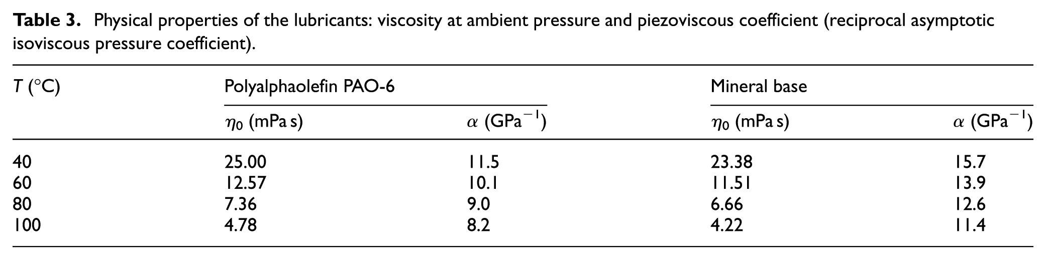
Two lubricants of different nature have been tested: a polyalphaolefin PAO-6 and a mineral base, whose physical properties were obtained from measurements in the laboratory and are presented in Table 3. These are lubricants of similar viscosities at ambient pressure, from which the same temperature-viscosity coefficient β = 0.033 K⁻¹ is obtained for both lubricants, but they present different piezoviscous and pseudoplastic behaviours. The following parameters of the Carreau model and thermal conductivity at 80°C are given in Echávarri et al. ²⁵ and Larsson and Andersson: ³⁸ n = 0.81, G = 0.1 MPa, K_l = 0.15 W/(m K) for the PAO-6 and n = 0.50, G = 1.0 MPa, K_l = 0.12 W/(m K) for the mineral base.

Table 3.

Physical properties of the lubricants: viscosity at ambient pressure and piezoviscous coefficient (reciprocal asymptotic isoviscous pressure coefficient).

T (°C)	Polyalphaolefin PAO-6		Mineral base
	η0 (mPa s)	α (GPa−1)	η0 (mPa s)	α (GPa−1)
40	25.00	11.5	23.38	15.7
60	12.57	10.1	11.51	13.9
80	7.36	9.0	6.66	12.6
100	4.78	8.2	4.22	11.4

The selected testing conditions are as follows: bath temperature 80°C, average velocities between 10 and 2000 mm/s, and SRR = 25% and 100%. The loads employed in the MTM are 20 and 28 N, which correspond to Hertz maximum pressures of 826 and 924 MPa, respectively; in the MPR, the load used is 100 N/mm, equivalent to 863 MPa.

In all cases, the contact tested is steel on steel, which presents a Young’s modulus of 210 GPa, with Poisson’s ratio 0.3, thermal conductivity of 41 W/(m K), density of 7850 kg/m³ and specific heat of 418 J/(kg K). Prior tests at very low velocity, corresponding to a specific film thickness tending to zero, have provided a boundary friction coefficient value around 0.13 for both lubricants, which is in the order of magnitude indicated in the previous studies^4,29,30 and in line with Zhu and Hu ¹¹ for highly polished samples, as in the case of those employed in our tests. Specifically, the combined roughness (RMS) results in 15 nm in the ball-on-disc contact of the MTM and 40 nm in the contact between discs of the MPR.

As already mentioned, the film thickness can be approached as constant ⁷ and it is computed for the total load W_T following the process outlined in Table 4. The Newtonian central film thickness at bath temperature, h_Ncb, is calculated according to the equations in Table 1. This result, when multiplied by the thermal factor φ_t in equation (15), gives a corrected value that corresponds to the Newtonian central film thickness at inlet temperature, h_Nct. At this point, we can determine the inlet temperature using equations (17) and (18). Later on, equation (14) is employed to take account of the shear-thinning effects and obtain the non-Newtonian central film thickness at inlet temperature, h_c. Thus, specific lubricant film thickness λ may be calculated by applying equation (1).

Table 4.

Calculation procedure for the film thickness.

Step	Description of the parameter calculated	Equations/tables
1	Newtonian central film thickness at bath temperature, hNcb = hNc(Tb)	Table 1
2	Thermal factor at bath temperature, φt(Tb)	Equation (15)
3	Newtonian central film thickness at inlet temperature, hNct	hNct = φt(Tb)·hNcb
4	Inlet lubricant temperature, Tin	Equations (17) and (18)
5	Non-Newtonian central film thickness at inlet temperature, hc(Tin)	Equation (14)

The calculation of the elastohydrodynamic friction coefficient is performed for the load supported by the lubricant film W_L. After calculating inlet temperature and non-Newtonian central film thickness as outlined in Table 4, an iterative process must be performed following the steps summarised in Table 5.

Table 5.

Calculation procedure for the friction coefficient.

Step	Description	Equations/tables
1	Hypothesis for the contact temperature	–
2	Viscous properties at contact temperature	Table 3
3	Fluid film friction coefficient	Equations (11–13)
4	Friction coefficient under mixed lubrication	Equation (6)
5	Determination of flash temperature	Equation (19), Table 2
6	Calculation of the contact temperature	Equation (16)

Starting from a hypothesis for the contact temperature, the viscous properties of the lubricant at this temperature can be obtained using Table 3, as well as the fluid film friction coefficient with the equations (11)–(13). Combining this result with the boundary friction coefficient, equation (6) gives an initial value of the friction coefficient under mixed lubrication. Later on, the flash temperature can be deduced using equation (19) and the formulae in Table 2, which, when added to the inlet temperature obtained previously, leads to a calculated value of the contact temperature according to equation (16). This result lets the initial hypothesis be verified. The contact temperature obtained in step 6 of Table 5 is compared to the hypothesis in step 1, and steps 1–6 are repeated until convergence, reaching this way the solution of both the contact temperature and the friction coefficient under mixed lubrication.

The theoretical results of friction obtained are compared with the experimental data in the following section, which also includes a discussion of the results.

It is worth highlighting that this article focuses on point and line contacts; and in the corresponding equations. However, the process is also applicable to other geometries, such as the elliptical. For this geometry, due to the lack of specific expressions, it is possible to use the results of load distribution functions by Zhu and Hu (7) or Castro and Seabra (8) as the results are quite close. Stachowiak and Batchelor ² provide the equations to obtain the central film thickness for an elliptical contact, while the point contact equations are applicable for calculating the effective pressure (12) and the inlet temperature (17). The flash temperature can be approximated to the Jaeger results for square- and band-shaped interfaces ³⁶ and the equations developed in Bansal and Streator ³⁹ can be used for greater precision.

Results and discussion

Figure 4 shows the results of the model for the two lubricants at a bath temperature of 80°C, in a point contact with a load of 20 N, an SRR of 25% and a broad range of average velocities that result in all lubrication regimes in the Stribeck curve. Given the increasing relation between the specific film thickness and the average velocity, also shown in this figure, in this section we represent the friction coefficient versus average velocity for greater clarity. In this way, it can be checked that the results of the model are in line with those published by other authors ¹⁷ and allow comparisons with experimental data.

Figure 4.

Theoretical results for the PAO-6 and the mineral base in a point contact.

Figure 4 shows that fluid film lubrication is attained at the highest velocities represented on the graph (λ > 2), where the greater viscous properties of the mineral base facilitate the creation of the film and involve a higher friction coefficient than PAO-6. Another consequence of the higher viscosity of the mineral base is its greater range of fluid film operation, as the transition towards a mixed regime (λ < 2) appears at lower velocities. It is worth noting that the friction curves of both lubricants tend towards the boundary friction coefficient as velocity is reduced.

A broad range of velocities has been selected in order to experimentally check the theoretical results, which includes different lubrication regimes. The data obtained from MTM are depicted in Figure 5, which compared with the results of the model show a good correlation for both lubricants.

Figure 5.

Comparison between theoretical and experimental results in a point contact at 80°C, 20 N and SRR = 25%.

The following analyses the behaviour of the model under different operating conditions, comparing the results with new tests in the MTM. Figure 6 shows some examples of good predictions found both on modifying the SRR and changing the normal load.

Figure 6.

Analysis of the correlation between theoretical and experimental results for a point contact lubricated with PAO-6 at 80°C in different operating conditions.

For an SRR of 25%, an increase in load from 20 to 28 N reduces the thickness of the lubricant film, resulting in greater weight of the boundary component of the friction coefficient and the subsequent increase in friction under mixed lubrication regime. In addition, the elastohydrodynamic friction is also increased by load due to the considerable influence of the piezoviscous effect, providing an additional increase in the friction coefficient, which is especially relevant for high average velocities.

If instead of increasing load, we increase SRR from 25% to 100%, the result is an increase of pseudoplastic and thermal effects that lead to the reduction of viscosity and film thickness, causing again an increase in friction due to the greater weight of the boundary component in mixed lubrication. Moreover, the rise in SRR causes the increase in sliding velocity and hence the shear stress and elastohydrodynamic friction. This effect is more pronounced at higher average velocities, but is mitigated by the aforementioned losses in viscosity.

Figure 7 provides contact temperature estimates, which show the important effect of the SRR on temperature. In addition, all curves increase as average velocity rises at a constant SRR, because of the proportional increase of sliding velocity. The greater the sliding velocity (or equivalently SRR), the greater the heat generation and therefore the temperature rises significantly.

Figure 7.

Contact temperature in a point contact lubricated with PAO-6 at 80°C in different operating conditions.

In addition to the effect of the sliding velocity, the friction coefficient influences the temperature reached in the contact. Figure 7 shows that the highest average velocities cause a more pronounced rise in temperature, as they correspond to a region where the friction coefficient grows with average velocity (Figure 6).

Likewise, the model can be used to predict the friction coefficient in line contacts and Figure 8 shows good agreement with experimental results in the MPR. In this case, complete fluid film lubrication is not achieved as velocity rises because of the greater roughness of the samples. The cases shown include different SRR values, with the subsequent variation in contact temperature, represented in Figure 9, and which displays an analogous behaviour to that of the point case.

Figure 8.

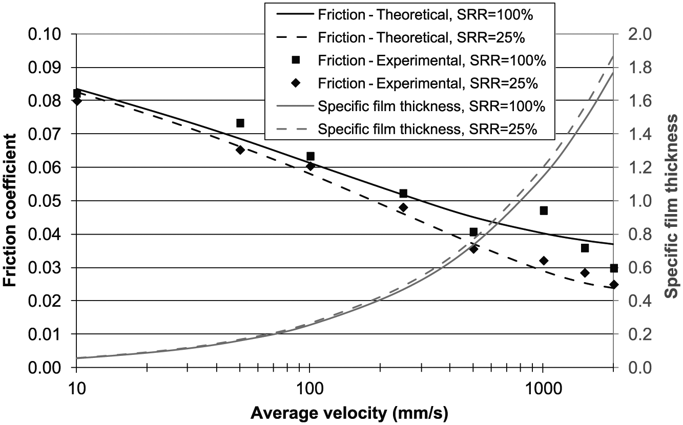
Analysis of the correlation between theoretical and experimental results for a line contact lubricated with PAO-6 at 80°C and 100 N/mm for different SRRs.

Figure 9.

Contact temperature in a line contact lubricated with PAO-6 at 80°C and 100 N/mm for different SRRs.

In summary, our simplified approach allows calculating reasonable predictions for a broad range of working conditions under highly loaded non-conformal contacts. This methodology offers practical utility as it is based on simple estimates of central film thickness and contact temperature, which lead to quick friction calculations.

The consideration of other rheological models that take into account other factors of influence, such as more complex pressure–viscosity behaviour based on free volume theory, can improve the accuracy of the results, particularly as Hertz pressures increase, but that would imply more tedious calculations and the need to introduce numerical algorithms. In addition to greater precision, another advantage of numerical simulations is that they provide complete distributions of film thickness and temperature, instead of approximate average values.

Nevertheless, the high complexity of numerical calculations often limits their practical use for engineering applications, as they require specific software, highly qualified personnel and considerable computational cost. Instead, analytical calculation can be performed quickly with the help of a simple spreadsheet, which makes it especially suitable for pre-modelling applications and in general to obtain approximate solutions for complex problems in the mixed lubrication regime.

Conclusion

A mixed lubrication model has been presented for highly loaded non-conformal contacts, based on a simplified analytical procedure that considers the thermal effects in the contact and the rheology of the lubricant. The procedure described has shown its capacity to estimate the friction coefficient in a simple way with reasonable precision for different lubricants and operating conditions, both for point and line contact. Simultaneously, it allows predicting specific film thickness and average contact temperature, which improves the analysis of the quantitative influence of the physical phenomena involved and contributes to a better understanding of the results.