Sage Journals: Discover world-class research

Abstract

Rolling element bearings and gears are the most common machine elements. As they are extensively used in rotating machinery, their health conditions are crucial to the safe operation. The signals measured from rotating machines are usually affected by the working conditions and background noises. Thus, identifying faults from the mixed signals is a challenging and important task. Deep learning is initially developed for image recognition. Recently, it has attracted increasing attention in machinery fault diagnosis research. However, the generalization ability of the default classifier of it is not very satisfying. Thus, combining the feature learning ability of deep learning and the existing classifiers with satisfactory generalization ability is necessary. In this article, a hybrid technique based on convolutional neural network and support vector regression is proposed. The former part is used to promote feature extraction capability, and the latter part is used for multi-class classification. The efficiency of the proposed scheme is validated using the real acoustic signals measured from locomotive bearings and vibration signals measured from the automobile transmission gearbox. Results confirm that the method proposed is able to capture fault characteristics from the raw data, and both bearing faults and gear faults can be detected successfully.

Keywords

Feature learning fault diagnosis convolution neural network support vector regression rotating machinery

Introduction

The rotating elements such as bearings and gears are the essential parts of the rotary machine. Their health conditions influence the running state of these machines significantly. Rolling bearings and gears, which are the most fundamental and important elements of rotating machinery, are widely used in various industrial machines and are thus usually subjected to harsh working conditions. The faults of bearings and gears often cause machine breakdown, which subsequently stops the production and leads to catastrophic economic loss or even a disaster, so fault diagnosis is a challenging problem that has been continuously studied.^1,2 The efficiency of fault diagnosis plays a highly consequential role in increasing the stabilization and the reliability of machinery and preventing catastrophes. Consequently, improving the methods for mechanical fault diagnosis has attracted considerable attention. Various condition-monitoring techniques, either through traditional signal processing algorithms or through newly up-to-date algorithms, are thus continuously produced.^3,4

Traditional algorithms ordinarily include the following three essential processes: feature extraction, selection of sensitive fault feature, and identification of the fault pattern.⁵ Feature extraction is the basis of fault diagnosis methods and is generally the first step in traditional algorithm.⁶ Typically, the features extracted are statistical parameters. The dimensions of these parameters should be reduced so that the parameter can be processed further. In this regard, the principal component analysis (PCA) is one of the primary strategies that reduces dimensions as well as an unsupervised dimension reduction algorithm. Yang and Wu⁷ employed PCA for the selection of a few significant principal components to present the dominated gears’ nature. The results showed that PCA can simultaneously enhance the diagnosis accuracy and reduce the feature. Six types of gear faults were used to verify the proposed method and showed that the PCA process exhibited a high accuracy in diagnosis and enhanced the computational efficiency of the artificial neural network (ANN). PCA was also used by Jiang et al.⁸ when they presented the Gaussian mixture model and optimal principal components–based Bayesian method to generate lower dimension and be more efficient evidence. The former studies indicate that PCA generally serves as a fundamental method and research on it is significant. Other frequently used methods for the reduction of feature dimensions are the independent component analysis (ICA) and the distance evaluation technique (DET).⁹ Han et al.¹⁰ used ICA-based method to develop a fast algorithm which had a faster convergence speed and higher precision. That algorithm was integrated with the wavelet packet energy spectrum and can accurately recognize the slight damage and fracture of a bearing. Meanwhile, Guo et al.¹¹ proposed an adaptive fault diagnosis algorithm for rotating machinery. That method could acquire the segment of the signal which has the most demanded characteristics. These strategies are typically used to extract useful features, which can reflect the healthy state of the machine. Finally, the accuracy of the identification process for machine health conditions in the selected sensitive fault features can be further enhanced using diagnosis methods, such as wavelet transform, decision tree, and fuzzy logic. Classical methods based on wavelet theory have achieved considerable progresses in the last 20 years. Wavelets-based fault diagnosis methods including wavelet packet transform (WPT), discrete wavelet transform (DWT), and continuous wavelet transform (CWT) and their applications were already reviewed by Yan et al.¹²

Although the fault diagnosis methods based on signal processing work effectively under actual applications, these methods rely on diagnostic expertise. Fortunately, artificial intelligence–based fault diagnosis schemes can potentially address this problem.

Recently, machine learning has become a significant topic of research. Machine learning provides many intelligent tools that can perform recognition and diagnosis, and it does not rely on an assumption of data normality. Current intelligent methods include boosting,¹³ bagging, auto-encoder,^14,15 support vector machine (SVM),¹⁶ and deep learning,¹⁷ such as deep belief network (DBN).¹⁸

Studies on deep learning theory started to substantially increase after 2006. In this year, new age studies on deep learning were instigated when GE Hinton et al.¹⁹ published his famously article. Deep learning is a class of techniques that can be used to identify objects, and deep learning methods usually have several or even hundreds of hidden layers. From each layer, the features containing fault characteristic information can be extracted and collected and then used as the input for the subsequent layer.²⁰ An advantage of nonlinear relation between input and output is the automatic transformation of the feature with low dimension into a corresponding abstract representation with high dimension.²¹ Deep learning overcomes the reliance on prior knowledge for the extraction and selection of the suitable features and the diagnostic expertise. This automatic feature extraction capability can reduce the need for human labor and enhance the effectiveness and competitiveness of deep learning.

Convolutional neural network (CNN) is one of the principal models of deep learning.²² Traditional CNN belongs to supervised learning and is a forward pass neural network. It is normally trained by the back-propagation (BP) algorithm, which may be computed using a stochastic gradient descent (SGD) technique. In a CNN model, the units belonging to a map undergoes weight sharing, that is, they share the same filter bank. Weight sharing, which is the highpoint of CNN, is used to increase the calculation and efficiency. CNN can obtain higher-level features through its deep architecture which is stacked hierarchically layer-by-layer. Similar to ANN architectures, the last but one layer of CNN is a fully connected layer. CNN is extensively used in diverse domains, such as image classification,²³ speech recognition,²⁴ language understanding,²⁵ fault diagnosis,²⁶ and other application fields.²⁷ However, these classic CNN models usually use a softmax classifier, which has a common generalization ability, as its top layer.²⁸

The SVM and its extension support vector regression (SVR) are commonly used in machine learning. In 1995, Vapnik²⁹ introduced the supervised learning computational approach, SVM, to analyze data and recognize patterns. The SVM classification algorithm is a promising method because it has been successfully applied in various engineering fields, such as data mining and mechanical fault diagnosis. It has a powerful generalization capability even without a large number of samples. Jegadeeshwaran and Sugumaran³⁰ used descriptive statistical features and SVM for fault diagnosis of the automobile hydraulic break system. In that article, the statistical features were extracted first and then were selected in the order of importance by a decision tree, which needed much more additional work. Erfani et al.³¹ developed a hybrid model based on deep learning and a one-class SVM for high-dimensional and large-scale anomaly detection. In that article, the deep learning algorithms including the DBN and the auto encoder are studied. The one-class SVM-based hybrid model performed well but the one-class SVM had a limitation in the face of multi-class classification. Sun et al.³² predicted the life of a bearing using an SVR-based process. The vibration signal features were also selected first before input to the SVR, although the proposed method is applied to the actual bearing data with a good performance. Qin et al.³³ optimized the parameters of SVR by adopting the particle swarm optimization and they applied the optimized method to the prognostic of lithium-ion batteries degradation experiment data. The results showed the improvement of the robustness and generalizability from limited data to long-term prediction. As a summary, SVR, as a classifier, has shown its great generalization ability.

CNN has shown its powerful ability to extract information and useful features. But the default classifier, softmax classifier, has a common generalization ability while the SVR has a relatively better performance. So it is necessary and meaningful to carry out such a research on these two methods. Hence, a novel supervised intelligent fault detection technique combined with CNN and SVR is proposed. The former part of this new model is worked as a feature extractor and the latter part worked as a classifier. This hybrid architecture is constructed by replacing the top layer of the traditional CNN with an SVR classifier. The signals are first processed by the CNN to obtain the features, which are extracted from the last hidden layer of the CNN. The extracted features are then inputted to the SVR, which is situated at the top of the model for classification. The new model is applied to detect the fault patterns of real acoustic signals measured from locomotive bearings and vibration signals measured from a gearbox. The performances of the CNN and SVR have improved in rotating machine fault detection when they were combined. Compared with the results of fault recognition obtained by traditional CNN, the results confirm that the proposed method is able to obtain the generic underlying characteristics of the raw data and achieve a high accuracy for both bearing fault detection and gear fault detection.

The remainder of this article is organized as follows. In section “Theoretical background,” the basic theories of the CNN and the SVR are presented concisely. Section “Proposed hybrid method” presents the proposed hybrid structure in detail. The experimental validation tests using bearing and gearbox data sets and a comparison between the proposed method and the traditional CNN are demonstrated in section “Effectiveness of the proposed algorithm.” The conclusion is summarized in section “Conclusion.”

Theoretical background

CNN

The CNN is as a prominent deep architecture of deep learning. CNN includes multiple layers of representations. Due to this deep structure, CNN can automatically obtain the representation characteristic from the raw data through nonlinear transformations and approximate nonlinear functions.

A typical CNN structure consists of a feature extractor which is composed of several convolutional layers usually followed by pooling layers and a softmax classifier. The convolutional layer extracts signal features, whereas the pooling layer reduces the dimensions and thus further reduces the computation time. This architecture can attain a form of regularization by itself. The features extracted are then put into the top softmax layer for classification. The theoretical basis of automatic feature extraction is described in the following.

Feedforward process

The supervised multi-class problem which CNN is going to solve is described as follows: let $S \subset R$ and $Y \subset R$ be the two random variables, S and Y have the relation of $Y = f (S)$ . Given a sample ${(s_{i}, y_{i})}_{i = 1}^{n}$ from the joint distribution of S and Y, n is the number of training examples for an m-class problem. This supervised learning is aimed to learn a mapping $\hat{f} : S \to Y$ , which can minimize the expected loss. The squared-error loss function is defined in equation (1)

E^{i} = \frac{1}{2} \sum_{k = 1}^{m} {(y_{k}^{i} - t_{k}^{i})}^{2}

(1)

where $y_{k}^{i}$ is the kth corresponding target label of sample i, and $t_{k}^{i}$ is the similar value of the kth output-layer unit.

However, the space of hypotheses is restricted to some set F to minimize the set of all functions from S to Y easily

\hat{f} : \underset{f \subset F}{\arg min} E [Y, f (S)]

(2)

CNN solves equation (2) through several stages. In the first stage, S passes through a series of convolutional filters and simple non-linearity. Data S is first put into the convolutional layer, and each subsequent layer $s_{i}$ is computed from the former layer $s_{i - 1}$ in a convolutional layer as

s_{i} = ρ (v_{i})

(3)

v_{i} = W_{i} \cdot s_{i - 1} + b_{i}

(4)

where $W_{i}$ is the convolutional filters, $b_{i}$ is the bias, and $ρ$ is an activate function. In a multi-class problem, the output target value is typically be expressed as a vector, and only the output node belonging to the right class is positive. The rest of the output nodes are either zero or negative, depending on the choice of the output activation function. In this article, the activate function is the rectified linear unit (ReLU) function. The ReLU function is defined as $ρ (v) = \max (0, v)$ , and it is a kind of nonlinear function that can not only produce sparse features, but also achieve fast convergence in the deep model.³⁴ Eventually, each layer can be written as a sum of convolutions of the previous layer

s_{j}^{l} = ρ (\sum_{i \in M_{j}} W_{j}^{l} \cdot s_{i}^{l - 1} + b_{j}^{l})

(5)

M_j represents the jth layer map.

The second stage of the solving process is using a subsampling layer applied pooling function. The aim of the pooling layer is to merge features of the same semantics into a single feature. Through this merging, the dimensions are reduced. After pooling, although the size of the feature map is reduced, the number of feature maps is unchanged. The subsampling function is

s_{i}^{l} = ρ (β_{i}^{l} down (s_{i}^{l - 1}) + b_{i}^{l})

(6)

where down(·) represents a subsampling function; $β_{i}^{l}$ and $b_{i}^{l}$ are a multiplicative bias and an additive bias of the ith point of lth layer, respectively.

At the top of a classical CNN model, there are a fully connected layer and a softmax classifier. Figure 1 has shown the architecture of a classical CNN.

Figure 1.

Architecture of a CNN.

BP process

The optimization problem of CNN is highly nonconvex, and thus, the BP algorithm is usually implemented to compute gradients. In addition, the SGD is used to update the weights $W_{j}$ .³⁵

The errors calculated by BP from the network can be regarded as sensitivities. It is the gradient of each unit and is defined as follows

\frac{\partial E}{\partial b} = \frac{\partial E}{\partial v} \frac{\partial v}{\partial b} = δ

(7)

This is the key point of the back algorithm propagated from higher layers to lower layer. The calculations of the gradients for the lth layer (l < L) and layer L are shown in equation (8) and equation (9).

δ^{l} = {(W^{l + 1})}^{T} δ^{l + 1} \circ ρ^{'} (v^{l})

(8)

δ^{L} = ρ^{'} (v^{l}) \circ (y^{n} - t^{n})

(9)

where ∘ denotes the element-wise multiplication.

Then the weight can be updated using the $δ$ rule, in which the lth derivatives of error with respect to the weight is equal to the output product between the vector of inputs and the vector of sensitivities

W^{l + 1} = W^{l} - η \frac{\partial E}{\partial W^{l}}

(10)

\frac{\partial E}{\partial W^{l}} = s^{l - 1} (δ^{l})^{T}

(11)

where $η$ is the learning rate, and s is the output feature from CNN.

The BP algorithm is briefly described in the flowchart in Figure 2.

Figure 2.

The flowchart of the BP algorithm.

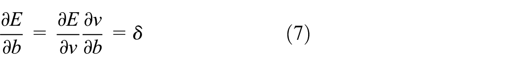
SVR

The SVR can be adopted as a multi-class classification strategy. In contrast to SVM, it can address multi-classification problems. The SVM is developed by Vapnik³⁶ and is proven to be an extremely robust and accurate supervised learning modus. Notably, the SVM has a fine theoretical foundation rooted in statistical learning theory. Nevertheless, the SVM is designed for two-class learning problems. It requires complementary strategies for multi-classification processes, and thus, the diagnosis becomes complicated. The SVR is an upgraded version of the SVM, and it is suitable to deal with the time series prediction. The theory of SVR is developed based on the basis of the SVM principles.³⁷

Let ${x_{i}, y_{i}}_{i = 1}^{n}$ be a training data set where $x_{i}$ is the extracted feature input from each original sample, n is the total number of samples, $y_{i} \in {1, 2, \dots, M}$ demonstrates the target class values, and M is the number of classes. The regressive function is defined as

f (x) = w \cdot x + b

(12)

where x is the support vector, w is the weight parameter representing the orientation of the hyperplane, and b is the bias, which means a scalar threshold.

The ε-insensitive function in equation (14) is introduced into the support vector model to promote a robust estimator insensitive to slight changes, such as ineffective performance due to the presence of outliers. A kernel strategy is used to deal with nonlinear tasks. Through the kernel function, data can be mapped to a feature space with higher dimensions, and then it can be regarded as linear. In this research, the kernel function is the radial basis function (RBF).³⁸ Its calculation formula is expressed as follows

K (x_{i} \cdot x) = \exp (- \frac{{‖ x_{i} - x ‖}^{2}}{2 σ^{2}})

(13)

where $σ$ represents a positive real number parameter.

{| ξ |}_{E} = {\begin{matrix} 0, & if | ξ | < ε \\ | ξ | - ε, & otherwise \end{matrix}

(14)

where $ε$ is an error limit.

The optimal problem of SVR is

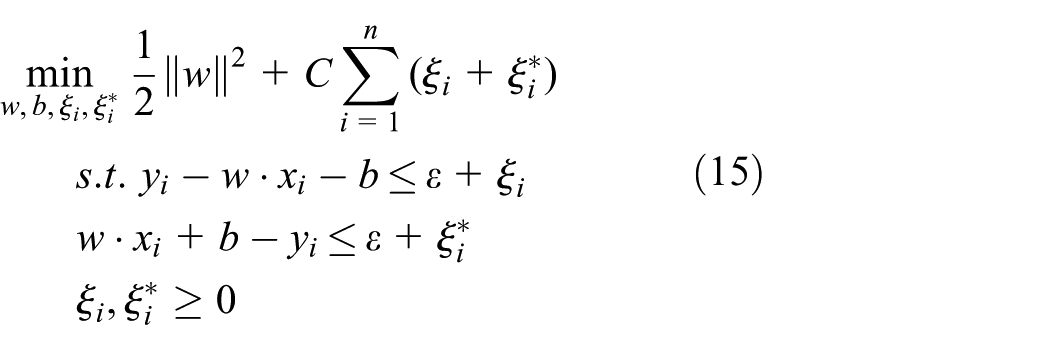
\begin{matrix} min_{w, b, ξ_{i}, ξ_{i}^{*}} \frac{1}{2} ‖ w ‖^{2} + C \sum_{i = 1}^{n} (ξ_{i} + ξ_{i}^{*}) \\ s . t . y_{i} - w \cdot x_{i} - b \leq ε + ξ_{i} \\ w \cdot x_{i} + b - y_{i} \leq ε + ξ_{i}^{*} \\ ξ_{i}, ξ_{i}^{*} \geq 0 \end{matrix}

(15)

where w is the weight vector, $‖ w ‖$ is its two-norm, b is the bias, C is a regularization parameter balancing the trade-off between the maximum margin and the minimum error, $ξ_{i}$ and $ξ_{i}^{*}$ indicate the slack variables, and $ε$ denotes the error limit.

The Lagrange multipliers are introduced to solve the previous problem. At this point, a Lagrange function is constructed as follows

\begin{matrix} L (w, b, α, α^{*}, ξ, ξ^{*}, μ, μ^{*}) \\ = \frac{1}{2} ‖ w ‖^{2} + C \sum_{i = 1}^{n} (ξ_{i} + ξ_{i}^{*}) - \sum_{i = 1}^{n} μ_{i} ξ_{i} - \sum_{i = 1}^{n} μ_{i}^{*} ξ_{i}^{*} \\ + \sum_{i = 1}^{n} α_{i} ((w \cdot x_{i} + b) - y_{i} - ε - ξ_{i}) \\ + \sum_{i = 1}^{n} α_{i}^{*} (y_{i} - (w \cdot x_{i} + b) - ε - ξ_{i}^{*}) \end{matrix}

(16)

where $α_{i}$ , ${α_{i}}^{*}$ , $μ_{i}$ , and $μ_{i}^{*}$ are the Lagrange multipliers.

Differentiating $L (w, b, α, α^{*}, ξ, ξ^{*}, μ, μ^{*})$ with respect to w, b, $ξ_{i}$ , and $ξ_{i}^{*}$ and setting the results equal to zero, then the parameters of optimality are obtained

{\begin{matrix} w = \sum_{i = 1}^{n} (α_{i}^{*} - α_{i}) x_{i} \\ \sum_{i = 1}^{n} (α_{i}^{*} - α_{i}) = 0 \\ C - α_{i} - μ_{i} = 0 \\ C - α_{i}^{*} - μ_{i}^{*} = 0 \end{matrix}

(17)

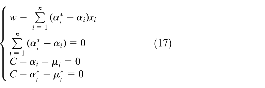
The problem becomes a convex quadratic programming optimization problem by substituting equation (17) into equation (16) and transforming the problem into its corresponding dual problem, as follows

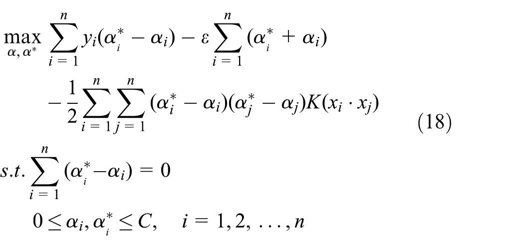
\begin{matrix} max_{α, α^{*}} \sum_{i = 1}^{n} y_{i} (α_{i}^{*} - α_{i}) - ε \sum_{i = 1}^{n} (α_{i}^{*} + α_{i}) \\ - \frac{1}{2} \sum_{i = 1}^{n} \sum_{j = 1}^{n} (α_{i}^{*} - α_{i}) (α_{j}^{*} - α_{j}) K (x_{i} \cdot x_{j}) \\ s . t . \sum_{i = 1}^{n} (α_{i}^{*} - α_{i}) = 0 \\ 0 \leq α_{i}, α_{i}^{*} \leq C, i = 1, 2, \dots, n \end{matrix}

(18)

The convex quadratic programming optimization problem in equation (18) can transform into a global optimum issue by adopting the sequential minimal optimization (SMO) algorithm which is an optimization technique.³⁹ Simultaneously, the Karush–Kuhn–Tucker (KKT) condition is satisfied. As a result, the convex optimization approach is a notable property of SVR. This approach ensures that a local solution is also the global optimum. That enables the SVR a better generalization ability which can achieve a high accuracy for the training and testing samples.

The f(x) which is the discriminate function that can predict the output $y_{i}$ with respect to the input $x_{i}$ within the error limit $ε$ then becomes

f (x) = \sum_{i = 1}^{n} (α_{i}^{*} - α_{i}) K (x_{i} \cdot x) + b

(19)

Based on the assumption that samples from the same pattern have similar outputs from the SVR, an SVR classifier can be constructed and the tested sample can be classified to class m when the tested sample satisfies the following function

\arg \min_{m = 1, 2, \dots, M} | m - (\sum_{i = 1}^{n} (α_{i} - α_{i}^{*}) K (x_{i} \cdot x) + b) |

(20)

Proposed hybrid method

The proposed hybrid model named CNN-SVR for fault diagnosis is a combination algorithm based on CNN and SVR theories. The CNN part is used as a feature extractor and the SVR as a classifier. In this model, constructing the hybrid architecture is the first step. During the construction, the top layer of the traditional CNN is replaced with an SVR classifier.

The new model is stacked layer-by-layer with convolutional layers and pooling layers inside. As shown in Figure 3, the structure combined of 10 layers totally, including the input layer, three convolutional layers, three pooling layers, two full-connected layers, and a support vector regressive classifier as the top layer.

Figure 3.

Structure of the hybrid CNN-SVR model.

In Figure 3, $D_{j}$ (j = 1, 2,…, 8) is the dimension of the number jth layer. Assuming that the sizes of convolution filter and pooling size are $(C_{i}, C_{i})$ and $(P_{i}, P_{i})$ (i = 1, 2, 3), the dimension of each layer is calculated according to the following functions

D_{j_{1}} = D_{j_{1} - 1} - C_{i} + 1, j_{1} = 2, 4, 6; i = 1, 2, 3

(21)

D_{j_{2}} = \frac{D_{j_{2} - 1}}{P_{i}}, j_{2} = 3, 5, 7; i = 1, 2, 3

(22)

D_{8} = n_{k} \times D_{7} \times D_{7}

(23)

where $n_{k}$ is the kernel number of the last convolutional or pooling layer, $D_{9}$ is the selected output dimension.

In the particular CNN-SVR model, the parameters are set as follows: the input layer size $D_{1}$ is 32, 5 filter kernels with size 5 × 5 for the first convolutional layer, 10 filter kernels with size 5 × 5 for the second convolutional layer, 10 filter kernels with size 2 × 2 for the third convolutional layer, the size of three pooling layers are all 2 × 2, and the size of the second full-connected layer set as D₉ = 100.

The raw signal from the data set is used as the input. At the start of the training stage, the raw data from the original data set are transformed into a matrix with several dimensions, and then the matrix is inputted to the visible first layer. The progress of the feature maps is the same as that defined in equation (5) of section “CNN.” The pooling layer next to the convolutional layer uses the max-pooling rule, that is, the pooling layer selects the largest coefficients over each sampling cell to reduce the dimensions by half. The feature map of the pooling layer is generated through equation (6) of section “CNN.” Other convolutional and pooling layers are constructed through the same procedures. The output from the last pooling layer is inputted to a full-connected layer with an output of 100 dimensions. Moreover, this output is used to extract features from the original signals. The learning process of this layer by layer-by-layer network can be reduplicated many times according to the requirement.

To specially note that in the proposed method, a sparse regularization penalty $φ (σ_{ij})$ is added to the final error function in the CNN part to decrease the number of parameters and the complexity of the computation. The sparse penalty can make a sparseness constraint on the distribution of the weights. Subsequently, the feature map which will be inputted to the SVR classifier can contain more useful information. The cost function and the update regulation of the weight described in equations (1) and (11) can then be adjusted into the following forms

{\tilde{E}}^{n} = E^{n} + \sum_{i, j} | σ_{ij} |

(24)

\frac{\partial \tilde{E}}{\partial W^{l}} = \frac{\partial E}{\partial W^{l}} + \frac{\partial φ}{\partial W^{l}}

(25)

Figure 4 shows the algorithm flowchart of this method. A summarized CNN-SVR algorithm involves the following steps:

Step 1. Input the data from the prepared data set and convert the signal vector into a matrix.

Step 2. Initialize the parameters, such as the total numbers of layers, the maximum epoch of iteration, the learning rate, the matrix of W, and the vector of b.

Step 3. Implement convolution and pooling.

Step 4. Fine-tune the stacked model using the optimized algorithm.

Step 5. Finish the optimization and acquire the features of the data set.

Step 6. Use the extracted features for classification by SVR.

Figure 4.

Algorithm flowchart of the CNN-SVR.

The fine-tune approach is conducted by the BP algorithm as described in section “BP process.” In detail, the supervised SGD is used to adjust the parameters of the hybrid model. Specifically, it first calculates the error between the output vector and the actual target vector, then obtains the loss function and the error of parameters. Using the SGD algorithm to get the gradients of the loss function and update the weights in corresponding layers. In addition, the SGD can further reduce the training error and promote the classification accuracy. In this study, stochastic gradient descent with mini-batches (MSGD) is accepted to make the learning process more efficiently.

In the proposed CNN-SVR model, the other related critical parameters are set as follows: the learning rate is 0.01, the total epoch iteration is 6000, and the mini-batch size is 100. The weight is randomly initialed and trained for optimization.

Effectiveness of the proposed algorithm

Experiment 1: locomotive bearing fault diagnosis

The rolling element bearing is the most common and essential component of rotating machinery. For the verification of the effectivity of this scheme, the bearing data measured from the locomotive are used.

Experiment equipment and data set

The rolling bearing data are obtained from an experimental platform, as shown in Figure 5. This experimental device consists of a laptop, a microphone, a testing bearing, a mechanical loading unit, a drive motor, a load display, a signal conditioner, and a data acquisition system (DAS). The bearing for testing is a kind of cylindrical roller bearing. Its type is NJ (P) 3226X1. It is mounted on the outer race. In its radial direction, an adjustable mechanical loading unit is installed.⁴⁰Table 1 lists the specifications of the bearing. The acoustic signals are collected through a 4944-A type microphone produced by the Brüel & Kjær Company (Copenhagen, Denmark). The microphone is placed near the bearing in a radial direction.

Figure 5.

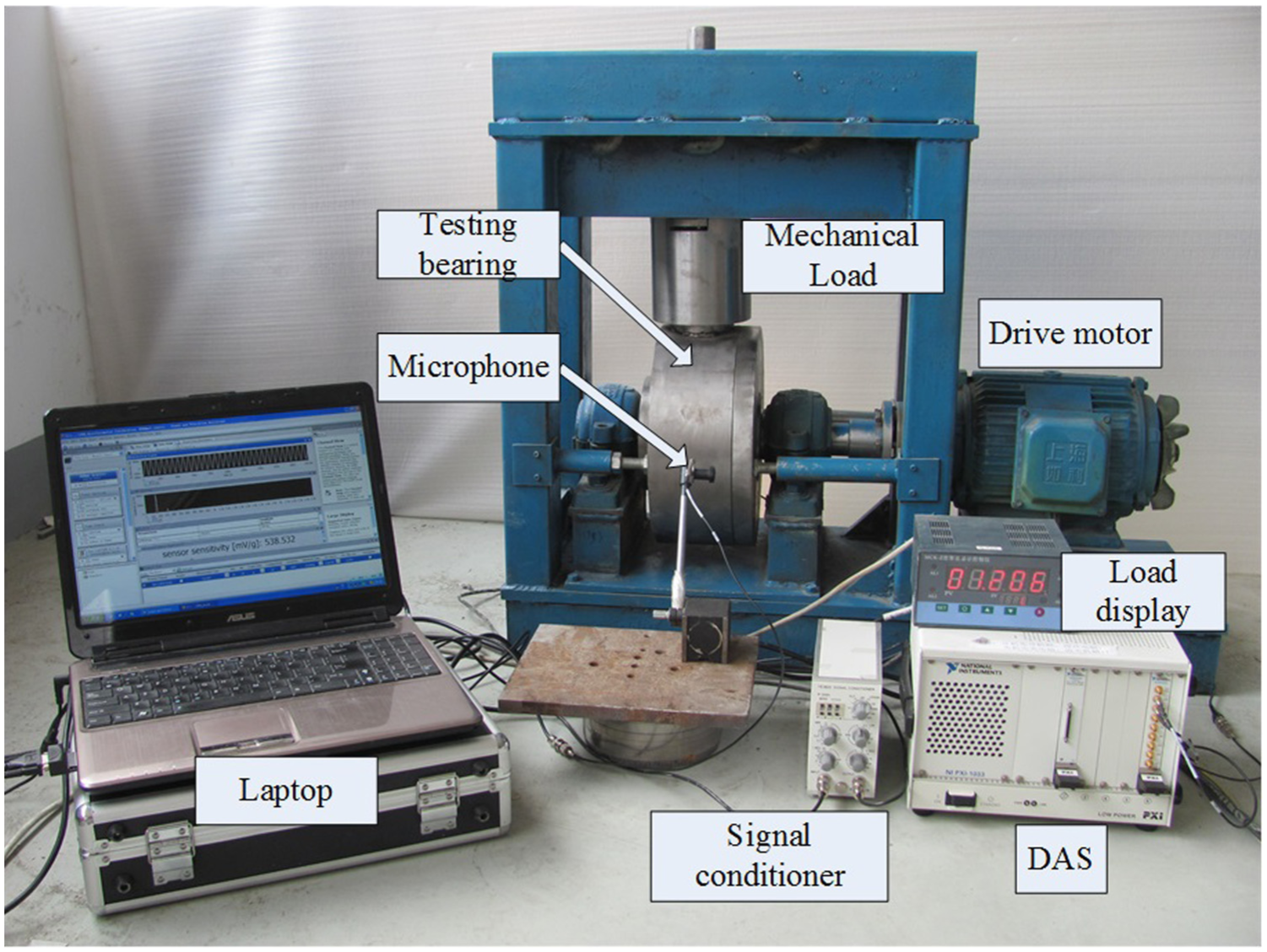
Experimental platform for bearing test.

Table 1.

Specifications of the testing bearing.

Item	Size (mm)/number
Outer race diameter	250
Inner race diameter	130
Pitch circle diameter	190
Rolling element diameter	32
Number of rolling elements	14

In this experiment, one normal bearing and three faulty bearings have been tested. The defect introduced into each faulty bearing is an artificial mark with a width of 0.18 mm. The defect is marked at the inner race, the outer race, and the rolling element, as shown in Figure 6. The collected acoustic signals were designated according to the kinds of rolling bearings, as follows: normal bearing (Norm), bearings with inner race fault (IF), rolling element fault (RF), and outer race fault (OF). All the signals are tested under the following conditions: rotor speed of 1430 r/min, 2.5 t loading, sampling frequency of 20 kHz, and sampling rate of 5000 points per second.

Figure 6.

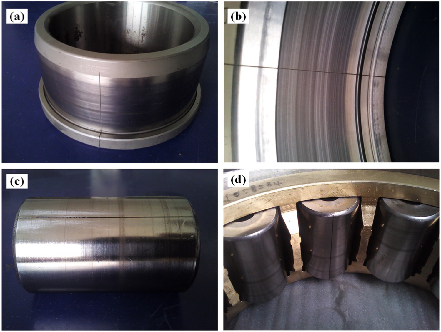
Defect setting of (a) inner race, (b) outer race, and (c, d) rolling element of the test bearing.

A group of experimental data constructed the Bearing Dataset. The composition of this data set is illustrated in Table 2. In total, 300 samples for each bearing condition are obtained. Of the 300 samples in each condition, 150 are selected randomly for training and 150 are selected for testing. Overall, 600 samples are used for training and 600 samples are used for testing.

Table 2.

Information of the Bearing Dataset.

Bearing status	Training	Testing	Output label
Norm	150	150	0
IF	150	150	1
RF	150	150	2
OF	150	150	3
Overall	600	600	0-3

Norm: normal bearing; IF: bearings with inner race fault; RF: rolling element fault; OF: outer race fault.

Diagnosis results

The time domain signals of different bearing statuses are shown in Figure 7. The differences among the four signal shapes are evident. However, distinguishing the condition of the bearing directly according to these variances is difficult. Therefore, the proposed method is used to analyze the fault patterns of the automotive bearing set.

Figure 7.

Acoustic signals of different bearing health conditions.

The current experiment is performed under different health conditions. The performance under each bearing condition is shown separately in Figures 8 –11 for clarity. Only two samples in the testing process of the normal bearing are misevaluated. All the other samples are categorized correctly both in training and testing processes. Moreover, the gather degree is quite higher. The average accuracy of the 10 times repetitions of the bearing data set is listed in Table 3. The average accuracies of the training and testing processes using the proposed method are both extremely high. Moreover, the accuracy of each condition is also listed in Table 3. The testing accuracy of the normal bearing is slightly lower. Nearly all of the data samples are classified correctly as indicated by the high accuracies. The new method not only digs generic fault characteristics of the rolling element bearings from different statuses adaptively but also exhibits a robust classification capability, thus producing good results.

Figure 8.

(a) Training and (b) testing results of normal bearing (Norm).

Figure 9.

(a) Training and (b) testing results of inner race faulty bearing (IF).

Figure 10.

(a) Training and (b) testing results of rolling element faulty bearing (RF).

Figure 11.

(a) Training and (b) testing results of outer race faulty bearing (OF).

Table 3.

Accuracy of different bearing conditions.

Method	Bearing status	Training (%)	Testing (%)
CNN-SVR	Norm	100	98.67
	IF	100	100
	RF	100	100
	OF	100	100
	Overall	100	99.67
CNN	Overall	99.5	97.66

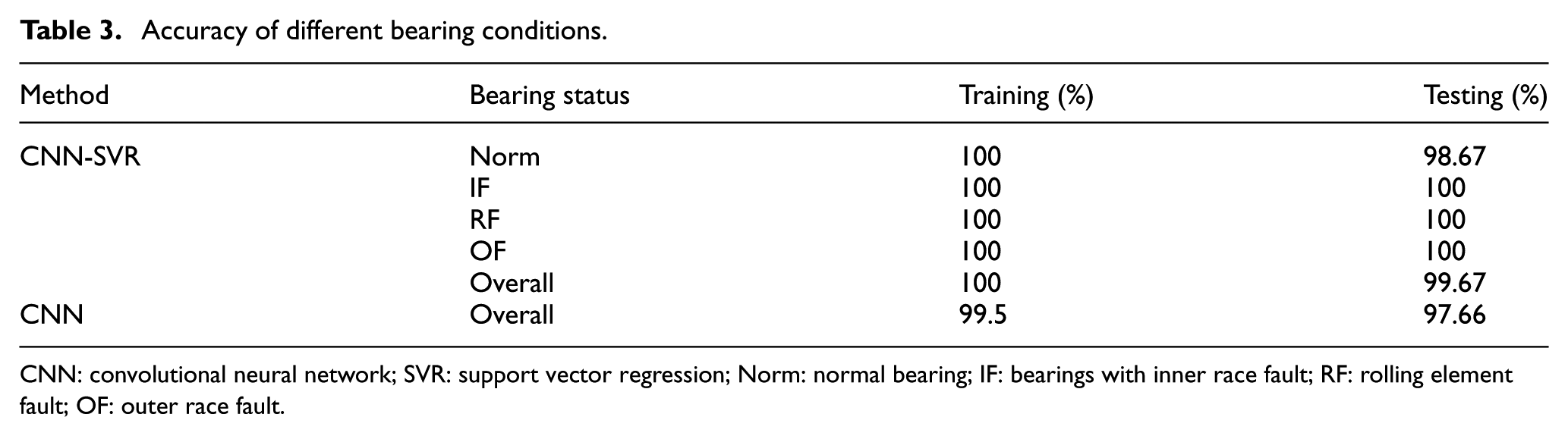
CNN: convolutional neural network; SVR: support vector regression; Norm: normal bearing; IF: bearings with inner race fault; RF: rolling element fault; OF: outer race fault.

For comparison, the traditional CNN, which contains a softmax layer as its classifier, is also used to deal with this data set. In addition, four bearing types, abbreviated as Norm, IF, RF, and OF correspondingly, are used. Similarly, half of the data are randomly selected for training and the other half are used for testing. The CNN has the same architecture as that of the proposed method, and thus, it can be trained using the same parameters. The accuracies of the training and testing processes are 99.5% and 97.66%, respectively, as shown in Table 3. The overall accuracies of the proposed technique are 100% for training and 99.67% for testing. For the visualization of the comparison, the diagnosis results of the training and testing processes using CNN are shown in Figures 12 and 13. The above results and comparison show that the new method can accurately identify the bearing fault categories and exhibits superior accuracy.

Figure 12.

Diagnosed results of training samples by CNN.

Figure 13.

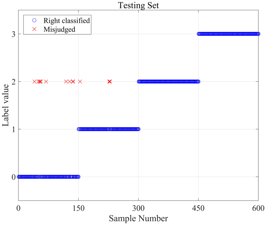
Diagnosed results of testing samples by CNN.

Experiment 2: automobile transmission gearbox fault detection

Experiment equipment and data set

The CNN-SVR algorithm is also validated using the gear fault data of an automobile transmission gearbox, as shown in Figure 14. The gearbox consists of one backward speed and five forward speeds. The vibration signals are measured by an accelerometer, which is mounted on the gearbox shell. The number three gears are used as testing gears for the wear process. The signals are measured during the forward motion of the automobile. The third gear teeth numbers of the driving gear and driven gear are 25 and 27, respectively. Their corresponding meshing frequency is 500 Hz. The rotating speed is 1600 r/min, and the sampling frequency is 3000 Hz. Five different running periods of the gearbox are listed in Table 4.

Figure 14.

Experimental platform for gear test.

Table 4.

Information of gearbox under different running periods.

Item	Status	Meshing times (thousand)
1	Running-in stage	0–700
2	Normal wear stage	700–2800
3	Slight wear stage	2800–5600
4	Medium wear stage	5600–6300
5	Broken tooth stage	6300–7000

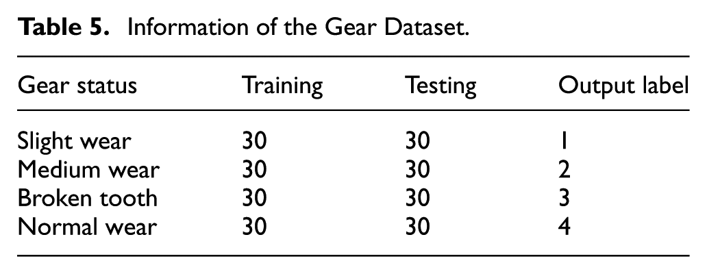
The Gear Dataset consists of four different status gear states. The four kinds of fault components are slight wear, medium wear, broken tooth, and normal wear, which are labeled as 1, 2, 3, and 4, respectively. Half of the samples in each condition is randomly selected for training and the other half is for testing. For each condition, the training and testing processes each uses 30 samples. The information of the Gear Dataset is shown in Table 5. The time domain signals of each gear state are shown in Figure 15. Judging the fault types directly from time domain signals is difficult.

Table 5.

Information of the Gear Dataset.

Gear status	Training	Testing	Output label
Slight wear	30	30	1
Medium wear	30	30	2
Broken tooth	30	30	3
Normal wear	30	30	4

Figure 15.

Vibration signal for different gear conditions: (a) slight wear, (b) medium wear, (c) broken tooth, and (d) normal wear.

Diagnosis results

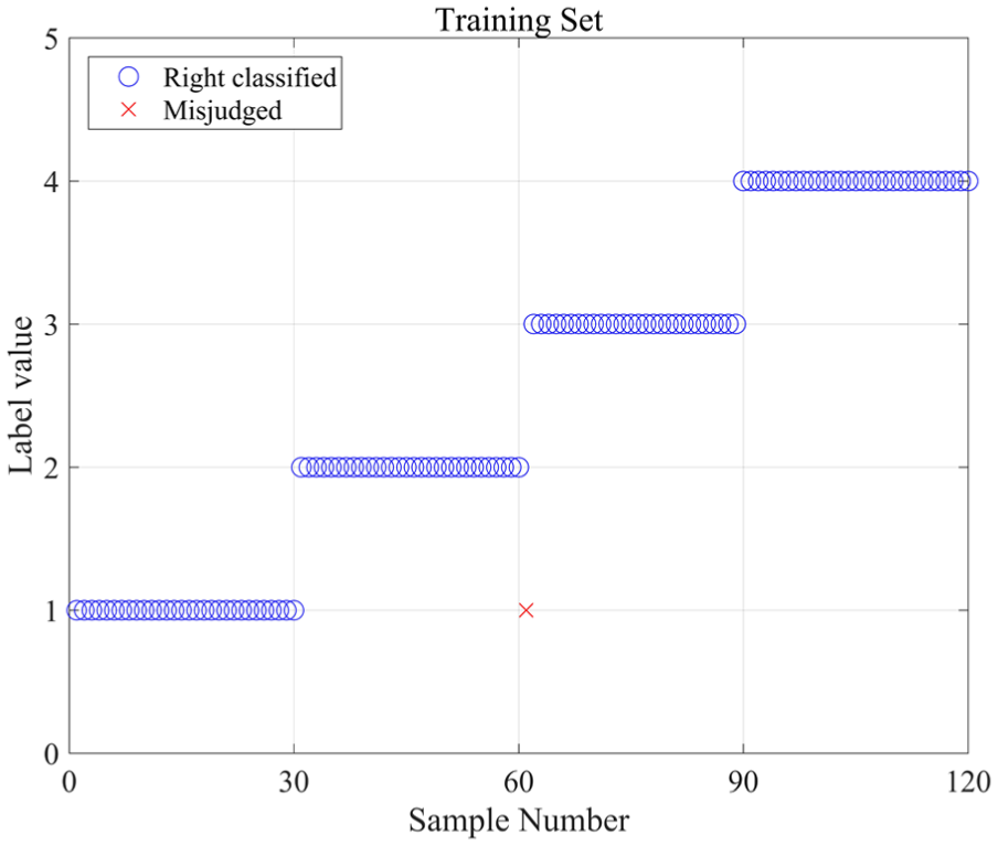
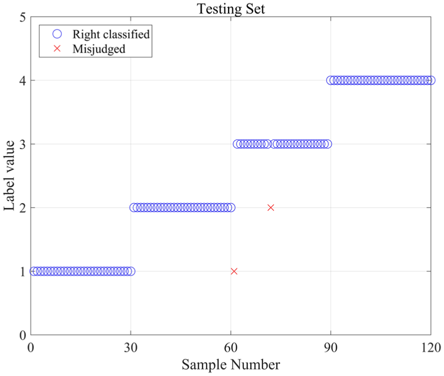
The diagnosis results obtained through the proposed algorithm are shown in Figures 16 and 17. All the samples of the training and testing processes are classified to the right fault type correctly. Although several samples are slightly decentralized from the actual label distribution, they have been judged to the right class eventually. This fine performance is mainly due to the generalization capability of SVR classifier. The overall accuracy is the average accuracy of 10-time repeats of this learning procedure. The average overall accuracies are 100% for both training and testing processes. The results imply that this model has a good ability to achieve high accuracy for gear fault diagnosis.

Figure 16.

The diagnosed results of training samples of Gear Dataset.

Figure 17.

The diagnosed results of testing samples of Gear Dataset.

Similarly, the traditional CNN using a softmax classifier is used to distinguish the fault types for algorithm comparison. The results are shown in Figures 18 and 19. The overall accuracies are 99.16% for the training process and 98.33% for the testing process. The contrast results of the separate conditions are also contrasted, as shown in Table 6. The results imply that both of these two methods can achieve a high accuracy when detecting the gear faults. The CNN-SVR model obtains a higher diagnosis accuracy and shows better robustness compared with the traditional CNN model.

Figure 18.

The diagnosed results of training process by CNN.

Figure 19.

The diagnosed results of testing process by CNN.

Table 6.

Accuracy of different gear conditions.

Gear status	Slight wear		Medium wear		Tooth broken		Normal
Gear status	Training (%)	Testing (%)	Training (%)	Testing (%)	Training (%)	Testing (%)	Training (%)	Testing (%)
CNN-SVR	100	100	100	100	100	100	100	100
CNN	100	100	100	100	96.67	93.33	100	100

CNN: convolutional neural network; SVR: support vector regression.

Conclusion

In this article, a hybrid intelligent technique based on CNN and SVR is proposed for fault pattern recognition in rotating machinery. This is a new combination of CNN and SVR which utilize the advantages of both methods. Then, from the raw time domain signals, features are extracted directly for the diagnosis of either bearings or gears. It saves a lot of manual work to extract and select the features and further accelerates the computation. Specifically, the effectiveness of the proposed fault diagnosis method is verified by both rolling element bearings data and gearbox data. The rolling bearing data are acoustic signals measured from real locomotive bearings, while the gear data are vibration signals measured from an automobile transmission gearbox. The results of the diagnosis show that CNN-SVR method is capable to extract the generic underlying characteristics from raw signal data. Moreover, this model can successfully distinguish the health status of the rotating elements. The validation results show that this new method can achieve a high precision for both the bearing fault diagnosis and the gear fault diagnosis. It is more accurate than the original CNN model. The good performance of the CNN-SVR method is mainly due to the superiority of the hybrid method, which combines the strong points of deep neural architecture and the powerful generalization of SVR. In summary, this hybrid technique has a good capability to extract useful features from raw time domain signals and exhibits a strong robustness in fault diagnosis. Last but not least, due to its ability to mine the fault characteristics from original time domain signals mechanically, the proposed approach does not rely on manual labor or the prior knowledge of signal processing manners and diagnostic expertise. Therefore, fault diagnosis applications of rotating machine can be achieved easier using the proposed method.

Footnotes

Acknowledgements

The authors would like to appreciate two anonymous reviewers for their constructive comments and suggestions.

Academic Editor: Dong Wang

Declaration of conflicting interests

The author(s) declared no potential conflicts of interest with respect to the research, authorship, and/or publication of this article.

Funding

The author(s) disclosed receipt of the following financial support for the research, authorship, and/or publication of this article: This research was financially supported by the National Natural Science Foundation of China (grant nos 51505311 and 51375322), the Natural Science Foundation of Jiangsu Province (no. BK20150339), and the Innovative Research Project for Postgraduates in Colleges of Jiangsu Province (project no. KYZZ16_0085).

References

Wang

Guo

Tse

PW.

An enhanced empirical mode decomposition method for blind component separation of a single-channel vibration signal mixture. J Vib Control 2016; 22: 2603–2618.

Wang

Huang

Gong

. Improved feature extraction using structured Fisher discrimination sparse coding scheme for machinery fault diagnosis. Adv Mech Eng 2016; 8: 1–16.

Zhang

Semisupervised distance-preserving self-organizing map for machine-defect detection and classification. IEEE T Instrum Meas 2013; 62: 869–879.

Wang

Guo

Xiaojuan

A joint sparse wavelet coefficient extraction and adaptive noise reduction method in recovery of weak bearing fault features from a multi-component signal mixture. Appl Soft Comput 2013; 13: 4097–4104.

Shen

Wang

Kong

. Fault diagnosis of rotating machinery based on the statistical parameters of wavelet packet paving and a generic support vector regressive classifier. Measurement 2013; 46: 1551–1564.

Ding

Sparse representation based on local time–frequency template matching for bearing transient fault feature extraction. J Sound Vib 2016; 370: 424–443.

Yang

TY.

Diagnostics of gear deterioration using EEMD approach and PCA process. Measurement 2015; 61: 75–87.

Jiang

Huang

Yan

GMM and optimal principal components-based Bayesian method for multimode fault diagnosis. Comput Chem Eng 2016; 84: 338–349.

Guo

. Envelope extraction based dimension reduction for independent component analysis in fault diagnosis of rolling element bearing. J Sound Vib 2014; 333: 2983–2994.

10.

Han

Guo

. Feature extraction method of bearing AE signal based on improved FAST-ICA and wavelet packet energy. Mech Syst Signal Pr 2015; 62: 91–99.

11.

Guo

Huang

Chen

. Elimination of end effects in local mean decomposition using spectral coherence and applications for rotating machinery. Digit Signal Process 2016; 55: 52–63.

12.

Yan

Gao

Chen

Wavelets for fault diagnosis of rotary machines: a review with applications. Signal Process 2014; 96: 1–15.

13.

Utkin

Zhuk

YA.

Robust boosting classification models with local sets of probability distributions. Knowl-Based Syst 2014; 61: 59–75.

14.

Sun

Shao

Zhao

. A sparse auto-encoder-based deep neural network approach for induction motor faults classification. Measurement 2016; 89: 171–178.

15.

Jia

Lei

Lin

. Deep neural networks: a promising tool for fault characteristic mining and intelligent diagnosis of rotating machinery with massive data. Mech Syst Signal Pr 2016; 73: 303–315.

16.

Liu

. Feature fusion using kernel joint approximate diagonalization of eigen-matrices for rolling bearing fault identification. J Sound Vib 2016; 385: 389–401.

17.

Längkvist

Karlsson

Loutfi

A review of unsupervised feature learning and deep learning for time-series modeling. Pattern Recogn Lett 2014; 42: 11–24.

18.

Sanchez

Zurita

. Gearbox fault diagnosis based on deep random forest fusion of acoustic and vibratory signals. Mech Syst Signal Pr 2016; 76: 283–293.

19.

Hinton

Salakhutdinov

Code

Reducing the dimensionality of data with neural networks. Science 2006; 313: 504–507.

20.

Gan

Wang

Zhu

Construction of hierarchical diagnosis network based on deep learning and its application in the fault pattern recognition of rolling element bearings. Mech Syst Signal Pr 2016; 72: 92–104.

21.

Shao

Jiang

Zhang

. Rolling bearing fault diagnosis using an optimization deep belief network. Meas Sci Technol 2016; 11: 115002.

22.

LeCun

Bengio

Hinton

Deep learning. Nature 2015; 521: 436–444.

23.

Krizhevsky

Sutskever

Hinton

GE.

ImageNet classification with deep convolutional neural networks. In: Proceedings of the advances in neural information processing systems, Harrahs and Harveys, Lake Tahoe, 3–6 December 2012, pp.1097–1105. Nevada: Curran Associates Inc.

24.

Sainath

Kingsbury

Saon

. Deep convolutional neural networks for large-scale speech tasks. Neural Networks 2015; 64: 39–48.

25.

Zhang

LeCun

Text Understanding from scratch. APL Mater 2015; 1710, https://arxiv.org/pdf/1502.01710.pdf

26.

Guo

Chen

Shen

Hierarchical adaptive deep convolution neural network and its application to bearing fault diagnosis. Measurement 2016; 93: 490–502.

27.

Yang

. 3D convolutional neural networks for human action recognition. IEEE T Pattern Anal 2013; 35: 221–231.

28.

Zhang

Bengio

Hardt

. Understanding deep learning requires rethinking generalization. arXiv:1611.03530, Toulon, France, 24–26 April 2017. ICLR.

29.

Vapnik

VN.

The nature of statistical learning theory. IEEE T Neural Networ 1995; 8: 1564.

30.

Jegadeeshwaran

Sugumaran

Fault diagnosis of automobile hydraulic brake system using statistical features and support vector machines. Mech Syst Signal Pr 2015; 52: 436–446.

31.

Erfani

Rajasegarar

Karunasekera

. High-dimensional and large-scale anomaly detection using a linear one-class SVM with deep learning. Pattern Recogn 2016; 58: 121–134.

32.

Sun

Zhang

Research on bearing life prediction based on support vector machine and its application. J Phys Conf Ser 2011; 305: 12028.

33.

Qin

Zeng

Guo

Robust prognostics for state of health estimation of lithium-ion batteries based on an improved PSO–SVR model. Microelectron Reliab 2015; 55: 1280–1284.

34.

Xing

Yang

Stacked denoise autoencoder based feature extraction and classification for hyperspectral images. J Sensor 2016; 2016: 3632943 (10 pp.).

35.

Mallat

Understanding deep convolutional networks. Philos T R Soc A 2065; 374: 20150203.

36.

Vapnik

VN.

Statistical learning theory. New York: Wiley, 1998.

37.

You

Yin

. An improved fault-location method for distribution system using wavelets and support vector regression. Int J Electr Power Energy Syst 2014; 55: 467–472.

38.

Pai

MC.

Dynamic output feedback RBF neural network sliding mode control for robust tracking and model following. Nonlinear Dyn 2015; 79: 1023–1033.

39.

Shigeo

Fusing sequential minimal optimization and Newton’s method for support vector training. Int J Mach Learn Cybern 2016; 7: 345–364.

40.

Shen

Liu

Wang

. A Doppler transient model based on the Laplace wavelet and spectrum correlation assessment for locomotive bearing fault diagnosis. Sensors 2013; 13: 15726–15746.

A hybrid technique based on convolutional neural network and support vector regression for intelligent diagnosis of rotating machinery

Abstract

Keywords

Introduction

Theoretical background

CNN

Feedforward process

BP process

SVR

Proposed hybrid method

Effectiveness of the proposed algorithm

Experiment 1: locomotive bearing fault diagnosis

Experiment equipment and data set

Diagnosis results

Experiment 2: automobile transmission gearbox fault detection

Experiment equipment and data set

Diagnosis results

Conclusion

Footnotes

Acknowledgements

Declaration of conflicting interests

Funding

References