A new fault feature for rolling bearing fault diagnosis under varying speed conditions

Abstract

Most fault detection methods based on the assumption of working in stationary or approximate stationary conditions are limited under varying operation conditions, for that the frequency aliasing phenomenon is inevitable in the spectrum. Therefore, in order to handle the problem of fault diagnosis under non-stationary conditions, researchers have proposed numerous methods and some achievements have been obtained. In this article, a new feature extraction method is proposed for fault diagnosis of rolling bearings under varying speed conditions. Based on the assumption that the energy will increase when balls cross over fault position, frequency values are divided by instantaneous speed and arranged in the descending order of corresponding amplitude to form a new fault feature array, that is, the ratio of frequency to instantaneous speed reconfiguration arrays. Thereafter, the Euclidean distance classifier is utilized for recognition. The efficacy of the proposed method is demonstrated by simulated and experimental data. Categorized results show that the new approach is capable of handling the bearing fault classification under varying speed conditions.

Introduction

Rolling bearings are widely used in rotating machines, and bearing failure is one of the most common causes of machine breakdown and accidents. ¹ Thus, it is important to study the defect diagnosis technology of rolling bearings. Vibration signals usually carry rich information about mechanical conditions and are often used to diagnose the faults of bearing’s localized defects.^2–4

During the past decades, many intelligent fault diagnosis approaches have been proposed to analyze vibration signals. Fast Fourier transform is the most common method proposed in Corinthios. ⁵ Theoretically, periodic impulses will be generated when the rolling elements pass over the defect in time domain and a distinct profile emerges on the frequency spectrum. However, in practice, it is much more complex, almost no machine can work under stationary condition.^4,6 Under varying operation conditions, the vibration signals collected from rolling bearing systems usually carry heavy background noise and the fault characteristic frequency is not only modulated as a series of harmonics but also is smeared on the frequency spectrum.^7,8 Therefore, existing techniques based on the assumption of working in stationary or approximate stationary condition such as FFT cannot work well in extracting the overwhelmed remarkable information for fault diagnosis. In order to solve this problem, researchers have proposed numerous methods based on time-frequency analysis (TFAs) and have made some achievements. However, each of these methods has its own limitation.

Short-time Fourier transform (STFT) was presented in 1947, ⁹ with a fixed length window function sliding along the time axis to intercept the signal into several segments. Corresponding frequency and amplitude variation along with time are obtained, but for the restriction of Heisenberg uncertainty principle,^10–12 the frequency and time resolutions may not be ideal at the same time. Wavelet transform (WT) was proposed in 1984 by Grossmann and Morlet, ¹³ which probably posed a considerable ideal resolution, for that the basic wavelet function can be modified according to the specific needs of specific applications. ¹⁰ According to different types of data analyzed, WT is divided into two classes, that is, continuous wavelet transform (CWT) and discrete wavelet transform (DWT), both of which have been developed successfully in the fault diagnosis field.^14–17 Whereas, selecting a suitable wavelet basis, which is the key to the successful application of this method, remains an open issue. ¹⁸ Empirical mode decomposition (EMD) was developed by Huang et al. ¹⁹ in 1998, decomposed a complicated signal into a few intrinsic mode functions (IMFs). And with higher time-frequency resolution, it has been widely used in mechanical fault diagnosis.^20–23 However, mode mixing as a major drawback may occur in EMD. Wigner Ville distribution (WVD) was proposed in 1948, ²⁴ though restricted by Heisenberg uncertainty principle, the time-frequency resolution has been greatly improved, the cross term is unavoidable in those techniques.^25–26

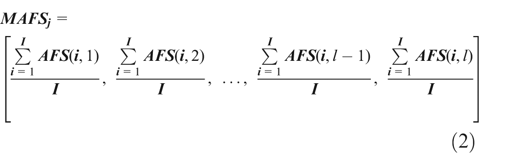
In view of the drawbacks existed in these methods, lots of improved methods had been presented. Although the shortage of these methods can be improved to some extent, they cannot be removed exactly. Considering these problems, this article presents a new fault feature extraction method based on the assumption that vibration produced by impacts has higher energy. First, the vibration signals collected from rotating machinery are intercepted with equal length randomly and processed by discrete-time Fourier transform (DTFT); second, the mean amplitude of each corresponding frequency values (AFS) of all arrays of frequency spectrums (MAFS) are calculated; repeat above steps to obtain multi-group MAFSs, and combine these results into a matrix in rows, then calculate the column mean of this matrix and get a row vector, which is called MMAFS; after that, MMAFS is sorted in descending order, and corresponding frequency values are ranked in the same sequence, these frequency arrays divided by instantaneous speed are the new fault features, named after the ratio of frequency to instantaneous speed reconfiguration arrays (RFISRA). In order to classify the faults of rolling bearings, RFISRA is calculated under different working conditions, respectively. Finally, the Euclidean distance classifier is utilized for recognition. The efficacy of the proposed method is demonstrated by simulated data and experiment signals. Categorized results show that the new approach is capable of handling rolling bearings fault classification.

The rest of this article is organized as follows: section “Feature extraction” details the process of feature extraction method proposed in this contest. In section “Simulation analysis,” a noisy fault simulated signal is formulated to validate the effectiveness of the proposed method. Section “Application to experimental signals” addresses the applications of the proposed method with the vibration signals from field tests. Finally, conclusions are drawn in section “Conclusion.”

Feature extraction

In spectrum analysis, when the spectrum amplitude of the target signal frequency is the maximum in spectrogram of the original signal, the identification effect of target signal is the best. ²⁷ Therefore, extracting appropriate impulse components as features is crucially important for fault diagnosis.

Thus, a new fault feature of the vibration signals called RFISRA is extracted and the construction process is shown in Figure 1. In this section, we will introduce the main steps of this construction process.

Figure 1.

Construction process of the RFISRA matrix.

Calculate the MAFS

Theoretically, the frequency components corresponding to the highest spectrum peak in the signal usually contains lots of useful information which can be assumed as the feature of the target signal. ²⁸ However, due to the disturbance of noise and interferences with higher energy, the assumption mentioned above may not be always correct.

In order to reduce the influence of noise and other interferences, the collected vibration signal $\mathit{x}(t)$ , which has the length of $\mathit{L}$ , be intercepted with the fixed length $\mathit{l}$ randomly, under the condition of $\mathit{L}>\mathit{l}\ge ({\mathit{f}}_s/min({\mathit{f}}_{re}))$ , the smaller the better, ${\mathit{f}}_S$ is the sampling rate and ${\mathit{f}}_{re}$ is the rotating frequency, then $x(t)=[x_1,x_2,\dots ,x_{i-1},x_i]$ , $\mathit{i}\le \mathit{I}$ is the number of signal segments, each signal segment ${\mathit{x}}_i=[{\mathit{x}}_i(1),{\mathit{x}}_i(2),\dots ,{\mathit{x}}_i(\mathit{l}-1),{\mathit{x}}_i(\mathit{l})]$ is changed from time to frequency by DTFT. The amplitude of frequency spectrum $\mathit{AF}{S}_i$ is calculated in equation (1), where ${\mathit{X}}_i$ is the DTFT of ${\mathit{x}}_i$

$$\mathit{AF}{S}_i=\frac{2\left|{\mathit{X}}_i\right|}{\mathit{l}}$$

(1)

Based on the above content, repeatedly intercept the signal for $\mathit{I}$ times and calculate the $\mathit{AF}{S}_i$ of those segments. Then combine them into a matrix $\mathit{AFS}=[{\mathit{AFS}}_1;{\mathit{AFS}}_2;\dots ;{\mathit{AFS}}_{\mathit{I}-1};{\mathit{AFS}}_{\mathit{I}}]$ , whose dimension is $\mathit{I}\times \mathit{l}$ . Then, the mean of each column of this matrix is calculated and a vector in the dimension of $1\times \mathit{l}$ is obtained as follows

$$\mathit{MAF}{\mathit{S}}_j=\left[\frac{{\displaystyle \sum _{i=1}^{\mathit{I}}\mathit{AFS}(\mathit{i},1)}}{\mathit{I}},\frac{{\displaystyle \sum _{i=1}^{\mathit{I}}\mathit{AFS}(\mathit{i},2)}}{\mathit{I}},\dots ,\frac{{\displaystyle \sum _{i=1}^{\mathit{I}}\mathit{AFS}(\mathit{i},\mathit{l}-1)}}{\mathit{I}},\frac{{\displaystyle \sum _{i=1}^{\mathit{I}}\mathit{AFS}(\mathit{i},\mathit{l})}}{\mathit{I}}\right]$$

(2)

Noise and other interferences are reduced by calculating the mean of amplitude spectrum to some extent.

Construct the MMAFS matrix and extract fault feature

Assume that the faults of $\mathit{p}-1$ type are going to be classified in rolling bearings. Besides, the normal condition should also be classified. Therefore, the considered health conditions of rolling bearings are $\mathit{p}$ types. Each of the vibration signals collected from different conditions should be analyzed. In order to eliminate the stochastic behavior and further reduce the noise and interferences disturbance, repeat the previous two steps for $\mathit{J}$ times, then a matrix with the dimension of $\mathit{J}\times \mathit{l}$ could be got as follows

$$\mathit{MAFS}=[{\mathit{MAFS}}_1;{\mathit{MAFS}}_2;\dots ;{\mathit{MAFS}}_{\mathit{J}-1};{\mathit{MAFS}}_{\mathit{J}}]$$

(3)

And a vector with the dimension of $1\times \mathit{l}$ is got after calculating the mean of each column of this matrix

$$\mathit{MMAF}{\mathit{S}}_k=\left[\frac{{\displaystyle \sum _{\mathit{j}=1}^{\mathit{J}}\mathit{MAFS}(\mathit{j},1)}}{\mathit{J}},\frac{{\displaystyle \sum _{\mathit{j}=1}^{\mathit{J}}\mathit{MAFS}(\mathit{j},2)}}{\mathit{J}},\dots ,\frac{{\displaystyle \sum _{\mathit{j}=1}^{\mathit{J}}\mathit{MAFS}(\mathit{j},\mathit{l}-1)}}{\mathit{J}},\frac{{\displaystyle \sum _{j=1}^{\mathit{J}}\mathit{MAFS}(\mathit{j},\mathit{l})}}{\mathit{J}}\right]$$

(4)

Furthermore, the above steps are repeated for $\mathit{K}$ times, then by combining these vectors into a matrix in rows, a matrix with the dimension of $\mathit{K}\times \mathit{l}$ is obtained

$$\mathit{MMAFS}=[{\mathit{MMAFS}}_1;{\mathit{MMAFS}}_2;\dots ;{\mathit{MMAFS}}_{\mathit{K}-1};{\mathit{MMAFS}}_{\mathit{K}}]$$

(5)

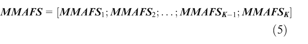
After that we sort the first half of these row vectors of this matrix in descending order, the corresponding frequency (single-side amplitude spectrum is considered here) is divided by instantaneous rotating frequency ${\mathit{f}}_{re}$ and ordered in the same sequence. Combining these frequency arrays into a matrix in rows, the new fault feature $\mathit{RFISRA}$ needed could be obtained.

In this section, the process of constructing a new fault feature is introduced to reduce the influence of noise and other interferences, and the length of signal segments $\mathit{l}\ge \frac{{\mathit{f}}_s}{min({\mathit{f}}_{re})}$ and the total number of repetitions satisfy the criterion of $\frac{\mathit{I}\times \mathit{J}\times K}{\mathit{L}-\mathit{l}}\ge 1$ , $\mathit{L}-\mathit{l}>\mathit{I}>1$ , $\mathit{J}>1$ , and $\mathit{K}>1$ . Figure 2 shows the proposed method in a flow chart.

Figure 2.

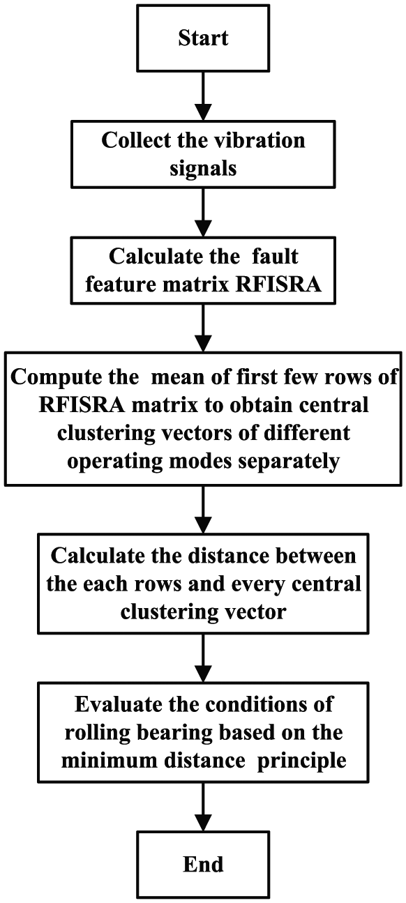
The complete process of the new method.

In order to verify the validity of the method, a simulated signal and experimental data are applied in sections “Simulation analysis” and “Application to experimental signals,” respectively.

Simulation analysis

In this section, a simulation study is conducted on a non-stationary signal which consists of both the Amplitude & Frequency modulated signal and the white Gaussian noise to verify the proposed method.

Simulation study

Considering the characteristics of the rolling bearing signals under varying speed, a synthetic signal $\mathit{x}(t)$ containing lots of different AM-FM components is constructed, each of the constituents can be written as

$${\mathit{x}}_{\mathit{i}}(t)={\mathit{s}}_{\mathit{i}}(t)+{\mathit{h}}_{\mathit{i}}(\mathit{t})+\mathit{n}(\mathit{t})$$

(6)

In these simulations, $\mathit{n}(t)$ is Gaussian noise; signal-to-noise ratio (SNR) is −8 dB; $\mathit{s}(t)$ and $\mathit{h}(t)$ represent a single impact signal and two harmonic signals, respectively; and they are defined as

$${\mathit{s}}_{\mathit{i}}(\mathit{t})={\mathit{A}}_{\mathit{i}}\exp (\beta /\sqrt{1-2{\beta }^2}\times \mathit{t})\times \cos (2\pi {\mathit{f}}_i{\mathit{f}}_{re}\times \mathit{t})$$

(7)

$${\mathit{h}}_{\mathit{i}}(\mathit{t})={\mathit{B}}_{\mathit{i}}\exp (\beta /\sqrt{1-2{\beta }^2}\times t)\times \sin (2\pi {\mathit{f}}_{\mathit{i}}^{\prime }{\mathit{f}}_{re}\times t)+{\mathit{C}}_{\mathit{i}}\exp (\beta /\sqrt{1-2{\beta }^2}\times t)\times \sin (2\pi {\mathit{f}}_{\mathit{i}}^{\prime \prime }{\mathit{f}}_{re}\times t)$$

(8)

where the structural damping ratio $\beta$ is 0.05; ${\mathit{A}}_i$ , ${\mathit{B}}_i$ , and ${\mathit{C}}_i$ are the amplitudes of impulses; ${\mathit{f}}_i$ , ${{\mathit{f}}_i}^{\prime }$ , and ${{\mathit{f}}_i}^{\prime \prime }$ are the structural parameters

$${\mathit{f}}_{re}=10+3t$$

(9)

And the sampling rate is ${\mathit{f}}_S=10\mathrm{kHz}$ , and the simulation time and sampling points are set as 1 s and $\mathit{L}=10,000$ .

In order to consider different working conditions, these coefficient values are presented in Table 1.

Table 1.

Coefficient values of simulated signals.

$i$	$A_i$	$B_i$	$C_i$	$f_i$	$f_i^{\prime }$	$f_i^{\prime \prime }$
$i=1$	7	4	1	10	50	70
$i=2$	6	3	9	40	20	80
$i=3$	2	8	5	90	60	30

Simulated signals are displayed in Figure 3.

Figure 3.

Simulated signals: (a) the waveform in time domain and (b) the DTFT of simulated signals.

Application of the method on simulated signal

After simulated signals being constructed, the new fault feature matrix with the method produced in section “Feature extraction” is extracted.

For the purpose of obtaining more accurate spectrum amplitude distribution, we set a fixed length of signal segment $\mathit{l}=1024$ , by arbitrarily selecting 50 sets from the possibilities, that is, $\mathit{I}=50$ , the sequence of DTFT spectrums ${\mathit{X}}_i$ can be obtained. Each ${\mathit{AFS}}_i$ of these segments is calculated with equation (1), then these ${\mathit{AFS}}_i\mathit{s}$ are combined into the $\mathit{AFS}$ matrix, which has a size of $50\times 1024$ . With equation (2), the ${\mathit{MAFS}}_j$ vector is calculated. Repeat the above steps for 50 times, that is, $\mathit{J}=50$ , 50 ${\mathit{MAFS}}_j$ vectors would be got, which would be combined into a matrix $\mathit{MAFS}$ with the dimension of $50\times 1024$ . The vector of ${\mathit{MMAFS}}_k$ is obtained with equation (4). Without loss of generality, repeat the prior steps for $\mathit{K}=100$ times, a matrix $\mathit{MMAFS}$ with a size of $100\times 1024$ is obtained. (Theoretically, the more segments we choose, the higher the precision we will get. By comparing and analyzing many experimental results under the requirement of improving calculation efficiency under precondition of assuring precision, we choose I  = 50, J  =50, K  = 100.) Each first half of row vector of the matrix is sorted in descending order and the corresponding frequency which has been divided by instantaneous rotating frequency ${\mathit{f}}_{re}=10+3\mathit{t}$ is ordered in the same sequence. After that, these frequency arrays are combined into a new fault feature matrix $\mathit{RFISRA}$ .

After calculating the fault feature matrices of different situations separately, classification would be made grounded on the Euclidean minimum distance. In order to realize recognition, the central clustering vector of each condition is obtained through computing the column mean of the first 50 rows of each matrix. The central clustering vectors of different simulated signals are shown in Figure 4.

Figure 4.

The central clustering vector of different simulated signals.

It can be found that the tendency of each end of these arrays has larger difference; therefore, the Euclidean distances of the rest vectors of these matrices to each central clustering vector of different situations are calculated, respectively. The identification results are classified according to the theory of minimum distance criterion. Here, the target output is defined as $\mathit{X}1=0$ , $\mathit{X}2=1$ , $\mathit{X}3=2$ . The classification results are shown in Figure 5.

Figure 5.

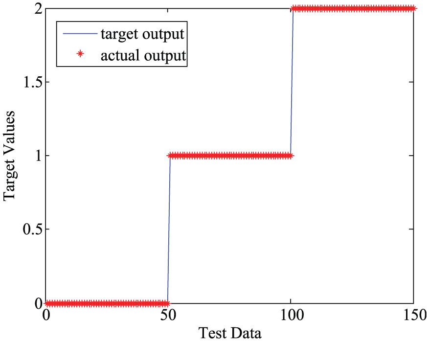
The result of simulated signal classification.

As can be seen in the picture, the classification accuracy of simulated signals reaches 100%.

To further investigate the effectiveness of the proposed detection method, the data provided from the Bearing Data Center of the Case Western Reserve University are explored. The test bunch is illustrated in Figure 6, the main components of the test stand include a 2 hp motor, a torque transducer (middle), a dynamometer (right), and a load motor connected by a self-aligning coupling. Single point faults were introduced to the test bearings with sizes of 7, 14, and 21 mils. Vibration data are collected with an accelerometer mounted on the motor housing at the drive end of the motor and the sampling frequency of each channel is 12 kHz.

Figure 6.

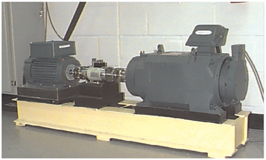
The test stand.

Application to experimental signals

In this article, the main focus are the faults of rolling bearings under varying speed conditions, so detailed descriptions of the analyzed dataset are provided in Table 2.

Table 2.

The details of different parameters.

Items	Normal				Fault
Fault size	0	7 mils			14 mils			21 mils
Fault location	None	IR	OR	RE	IR	OR	RE	IR	OR	RE
Motor speed	1797	1797	1797	1797	1797	1797	1797	1797	1797	1797
	1772	1772	1772	1772	1772	1772	1772	1772	1772	1772
	1750	1750	1750	1750	1750	1750	1750	1750	1750	1750
	1730	1730	1730	1730	1730	1730	1730	1730	1730	1730
Sample length, $\mathit{L}$	20,000	20,000	20,000	20,000	20,000	20,000	20,000	20,000	20,000	20,000
Segment length, $\mathit{l}$	4096	4096	4096	4096	4096	4096	4096	4096	4096	4096

IR: inner raceway; OR: outer raceway; RE: rolling elements.

First, we choose the data with the fault diameter of 7 mils, including inner raceway (IR), outer raceway (OR), and the rolling elements (RE), respectively. Each condition has the sample length of 20,000. Vibration signals are collected by an accelerometer with the sampling frequency of 12 kHz. In this article, faults are divided based on the minimum distance criterion, and the target outputs of classification is $\mathit{Normal}=0$ , $\mathit{Inner}=1$ , $\mathit{Ball}=2$ , and $\mathit{outer}=3$ .

The $\mathit{MMAFS}$ of different faults at the speed of 1797 r/min are calculated according to the steps introduced in section “Feature extraction” and combined into frequency matrices with the size of $100\times 2049$ , respectively. Then, they are divided by corresponding rotating frequency to get $\mathit{RFISRA}$ matrices. In this contest, the first 50 rows of each fault feature matrix are chosen to calculate the central clustering vectors under different faults modes. In order to be more convincing, the normal condition should also be considered. The results are shown in Figure 7

Figure 7.

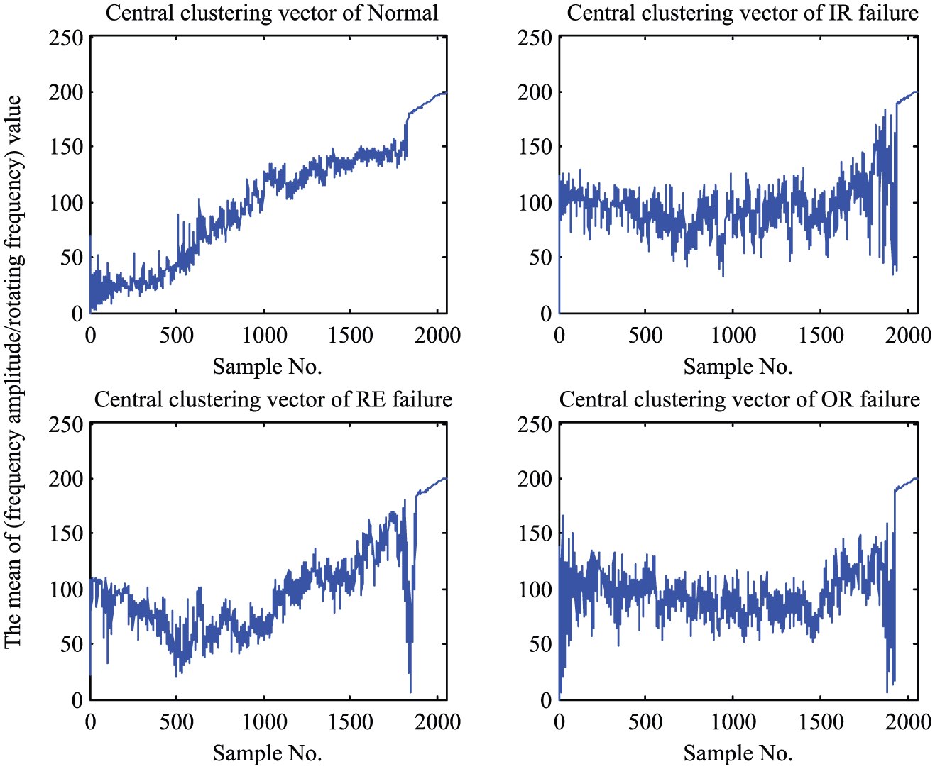
The central clustering vector of different experiment signals under the fault size of 7 mils.

As we can see, the central clustering vector of bearing operated under no fault maintains a sustained upward trend. However, when faults happen, the tendency appears to slip first and then rise up. The reason for such phenomena is that when faults happen under the condition with reduced noise and other interferences disturbance, in other words, the faults frequencies are the dominant components, with corresponding spectrum amplitudes increasing, the frequency is then sorted in the descending order of spectrum amplitudes, which causes the central clustering vectors slipping first and then rising up. Different faults have different frequency components, so corresponding central clustering vectors have special shapes as shown in Figure 7.

For the purpose of verifying the effectiveness of the method proposed in this contest under varying speed conditions, characteristic matrices of different forms in 1772, 1750, and 1730 r/min are calculated separately in the same way mentioned above, under the condition of bearing fault size being7 mils. Then, 12 matrices would be got and then they are combined with the last 50 rows of the $\mathit{RFISRA}$ matrices in 1797 r/min to form an unclassified matrix, which has a size of $1400\times 2049$ . Each row vector of this matrix is sorted by the minimum Euclidean distance between it and different central clustering vectors calculated above. The distinguishing results under the fault size of 7 mils are shown in Figure 8.

Figure 8.

Classification result under the fault size of 7 mils.

In the picture, it could be told that under the fault diameter of 7 mils, the fault recognition rate is 1374/1400, about 98.14% of the total. In detail, when the bearing is working under normal conditions, the rate is 100%, the same with the condition of ball fault and outer fault. But, under the condition of bearing with inner fault, 26 arrays are mis-recognized and the rate is 92.57%.

Under the fault diameter of 14 mils, the fault recognition rate is 1252/1400, about 89.43%. Different from the situation of 7 mils, the working conditions of normal, inner fault, and ball fault have 100% diagnosis accuracy. However, the diagnosis rate of bearing with outer fault is only 57.71%, that is, 202/350. The central clustering vector and classification result are shown in Figures 9 and 10, respectively.

Figure 9.

The central clustering vector of different experiment signals under the fault size of 14 mils.

Figure 10.

Classification result under the fault size of 14 mils.

As can be seen from Figures 11 and 12, under the fault diameter of 21 mils, the fault recognition rate is 1174/1400, about 83.86% of the total. Different from other cases, when the bearing approaches to failure, there are only two conditions namely normal and inner fault, the diagnosis rate keeps at 100%, the rate of outer fault is 311/350, about 88.86%, which is a little lower. But for the situation of ball fault, the rate is only 163/350, 46.57%, the method become invalid under this failure form.

Figure 11.

The central clustering vector of different experiment signals under the fault size of 21 mils.

Figure 12.

Classification result under the fault size of 21 mils.

As indicated above, we can come to the conclusion that the method proposed here have a good performance in dealing with the rolling bearing fault diagnosis under varying rotation speed. The rate of diagnosis of different conditions is shown in Table 3.

Table 3.

The rate of diagnosis of different conditions.

Items	Normal				Fault
Fault size	0	7 mils			14 mils			21 mils
Fault location	None	IR	OR	RE	IR	OR	RE	IR	OR	RE
Recognition rate	100%	100%	92.57%	100%	100%	57.71%	100%	100%	88.86%	46.57%
Rate in total		98.14%			89.43%			83.86%

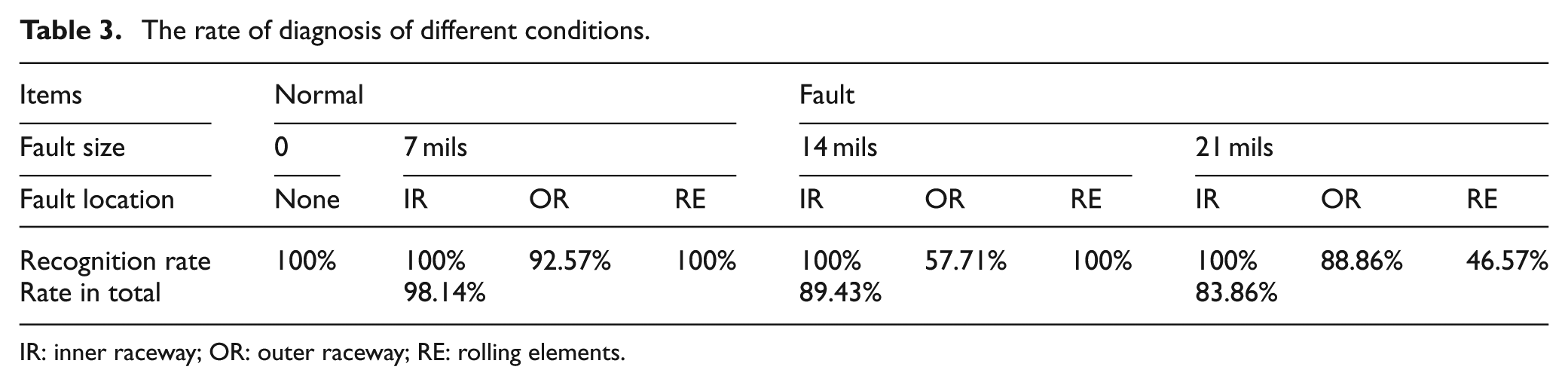
IR: inner raceway; OR: outer raceway; RE: rolling elements.

To illustrate the potential of the method proposed, Table 4 compares bearing fault type classification in this article with a few related studies using the same data.

Table 4.

Comparison with other methods under the fault diameter of 7 mils.

Literature	Classifier	Feature extraction method	Maximum accuracy
Zhao et al. 29	SVM	WPT and MPEWPD-PE	94.2%88.3%
Wang et al. 30	HMM	WPD	96%
Jiang et al. 31 and Zhu and Li 32	SVM	HE	98%
This study	ED	RFISRA	98.14%

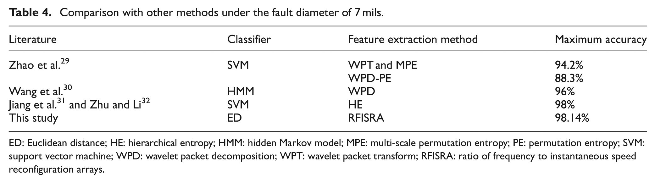
ED: Euclidean distance; HE: hierarchical entropy; HMM: hidden Markov model; MPE: multi-scale permutation entropy; PE: permutation entropy; SVM: support vector machine; WPD: wavelet packet decomposition; WPT: wavelet packet transform; RFISRA: ratio of frequency to instantaneous speed reconfiguration arrays.

Conclusion

In this context, a new fault feature of the rolling bearing vibration signals called $\mathrm{RFISRA}$ is extracted, the central clustering vectors of different conditions are calculated with it, and then the Euclidean distance classifier is utilized in recognition. The proposed method is demonstrated by simulated and experimental data, respectively. The main contributions of this article are summarized as follows:

1. The new fault feature $\mathit{RFISRA}$ is able to represent different fault forms of rolling bearings under varying speed conditions.

2. The multiple stochastic averaging is used to reduce the influence of noise and other interferences, and ensure accurate extraction of fault features under strong noisy environment.

3. Simulated and experimental signals demonstrate that the proposed method can avoid the difficulty of analyzing the frequency components, which is called frequency aliasing caused by speed variation. Compared with other methods, the proposed method presents a definite advantage.

We also notice that the results of classification reduce to some extent with the increase of fault size, such as 14 mils of “OR” and 21 mils of “RE.” In order to show that this phenomenon is not accidental, we use the method proposed in this article to identify different fault levels under the same speed condition, and classification results are shown in Figure 13.

Figure 13.

Classification result under different speeds.

We calculate the center vectors with the data collected under the fault diameter of 7 mils at different speeds, respectively. The data collected under the fault diameter of 14 and 21 mils are used as test data. The results show that the proposed method is effective in the inner fault identification, but failed in the outer fault and ball fault classification. It may be caused by the fact that the fault component will be blurred in noise more seriously with the fault degree increasing. Therefore, how to eliminate the interference and increase the intensity of useful signal on the basis of the proposed method should be further considered in future work.