Sage Journals: Discover world-class research

Abstract

The early recognition of wheel wear is an important task to the safe and efficient operation of a railway network. This article presents a new dictionary learning approach for wheel condition monitoring based on an adaptive parametric algorithm of blind source separation and extending K-means and singular value decomposition algorithm. Numerical simulations confirm the effectiveness of the proposed method. An experiment of wheel condition monitoring is conducted using a JD-1 wheel/rail simulation facility. Data calculation and theoretical analysis of wheel–rail contact dynamic show that the proposed method can adaptively learn and accurately identify wheel defects and verify the performance of the proposed method.

Keywords

Dictionary learning adaptive parameter blind source separation wheel condition monitoring

Introduction

Condition monitoring techniques of railway wheel wear have been researched globally for many years.^1,2 Broadly speaking, there are two types of monitoring system: infrastructure-based monitoring and rolling-stock-based monitoring. Infrastructure-based monitoring equipment, such as acoustic and vision sensors, is mainly set up at specific sections, and measurement speed is generally lower than the normal train speed.^3,4 This article examines rolling-stock-based monitoring based on vibration measurements made by accelerometers which detect wheel defect information produced by the impact of the wheel and rail. Vibration measurement is an important approach which is based on the idea that the wheel has specific vibration signatures under standard conditions and the signature changes with the development of the wheel wear, and the possible existing wheel defects can be recognized by signal processing techniques.⁵

However, signal analysis of wheel wear requires further improvement. It is a hard work to recognize wheel faults in the beginning stage, although eventually which can be detected by static measurement devices. A significant challenge is that the observation signal of wheel–rail interaction due to wheel wear is the mixture of the wear impact response signal and the regular wheel–rail contact vibration signal which overlap in time domain and frequency domain.⁶ Dictionary learning is an attractive tool in decomposing mixed signal components whose locations in time and frequency vary widely. This article presents a new dictionary learning approach for wheel condition monitoring.

During the last decade, dictionary learning has attracted a lot of attention in signal processing, machine learning, and compressive sensing of audio and visual data.⁷ The goal of dictionary learning is to decompose an observation signal into a linear expansion of some analytical bases, called atoms, that are selected from a large and, in general, redundant family of functions called a dictionary.⁸ Two of the most well-known dictionary learning algorithms are the method of optimal directions (MOD)⁹ and the K-means and singular value decomposition algorithm (K-SVD).¹⁰ Some approaches have been introduced to approximate the desired solution, such as greedy pursuit methods which iteratively refine the current estimate for the coefficient vector by modifying one or several coefficients chosen to yield a substantial improvement in approximating the signal. The relaxation methods also approximate the desired solution by replacing the combinatorial problem with a tractable one.¹¹ Greedy pursuit methods include orthogonal matching pursuit (OMP),¹² compressive sampling matching pursuit,¹³ subspace pursuit,¹⁴ and so on. Iterative shrinkage-thresholding,¹⁵ smoothed norm,¹⁶ and interior-point methods¹⁷ are some examples of the relaxation methods.

Effective study of these algorithms in recent years has established when the sought solution is sparse enough on a prespecified set of dictionary atoms: wavelets, Gabor bases, and more. The success of such dictionaries in applications depends on how suitable they are to sparsely describe the signals in question. Sparsity of observation signals is a prerequisite for classical dictionary learning methods. It can be very challenging as the signals are non-sparse in their current domain or transform domain.

Attempting to address the non-sparse problem, this article considers a different route for designing dictionary based on adaptive learning. A new dictionary learning method is proposed based on the adaptive parametric algorithm of blind source separation (ApBSS) and the extending K-SVD to exploit a dictionary by the observation signal itself. The proposed method consists of two steps: atoms extraction and dictionary representation. In the first step, the ApBSS is used to accurately extract sources from the observation signal, and a local dictionary is adaptively learned from sources. In the second step, the extending K-SVD is performed to compute the best decomposition of the signals, and representation patterns are updated to minimize the error according to given supports.

The remainder of the article is organized as follows. Section “Classical dictionary learning method” describes the principle and the limitation of conventional dictionary learning methods. In section “A new method of dictionary learning in blind source basis,” a new dictionary learning approach on blind source basis is proposed. Numerical simulations confirm its effectiveness. In section “Wheel condition monitoring,” an experiment of wheel condition monitoring is conducted using a JD-1 wheel/rail simulation facility. The results of data calculation and theoretical analysis of wheel–rail contact dynamic show that the proposed method can adaptively learn and accurately identify wheel defects and verify the performance of the proposed method. Section “Conclusion” summarizes the entire work.

Classical dictionary learning method

This section describes the procedure of dictionary learning from sparse approximation to signal recovery. Also, the limitation associated with conventional dictionary learning methods is illustrated by numerical simulations.

Using an overcomplete dictionary matrix $D \in ℝ^{n \times K}$ that contains K prototype atoms for columns ${d_{j}}, j = 1, \dots, K$ , an observation signal $y \in ℝ^{n}$ can be represented as a linear combination of these atoms. The vector $x \in ℝ^{K}$ contains the representation coefficients of the signal y . If $n < K$ and D is a full-rank matrix, the solution with the fewest number of nonzero coefficients is certainly an appealing representation. This sparsest representation is the solution of

(P_{0, \in}) min_{x} ‖ x ‖_{0} subject to ‖ y - D x ‖_{2} \leq \in

where $‖ \cdot ‖_{0}$ is the $l^{0}$ norm, counting the nonzero entries of a vector.

Exact determination of sparsest representations proves to be an NP-hard problem.^18,19 Approximate solutions are considered instead, and some efficient pursuit algorithms have been proposed. Among the existing methods for decomposing a signal in terms of dictionary atoms, OMP²⁰ is one of the most widely used approaches. It forms a $n \times K$ matrix D whose rows are the measurement vectors. The K measurements of the signal can be collected in a K-dimensional vector $v = D y$ . Since y has only m nonzero components, the data vector v is a linear combination of m columns from D. To identify the signal y , pick columns in a comprehensive fashion to determine which columns of D participate in the measurement vector v . At each iteration, the column of D that is most strongly correlated with the remaining part of v is chosen. Then its contribution to v is subtracted off. After m iterations, the algorithm is expected to identify the correct set of columns. The procedure of OMP is as follows:

Initialize the residual $r_{0} = v$ , the index set $Λ_{0} = 0$ , $D_{t} = \emptyset$ , and the iteration counter $t = 1$ .

Find the index $λ_{t}$ that solves the optimization problem $λ_{t} = argma x_{j = 1, \dots, K} | 〈 r_{t - 1}, d_{j} 〉 |$ . If the maximum occurs for multiple indices, break the tie deterministically.

Augment the index set and the matrix of chosen atoms

Λ_{t} = Λ_{t - 1} \cup {λ_{t}} and D_{t} = [\begin{matrix} D_{t - 1} & d_{λ_{t}} \end{matrix}] .

Solve a least squares problem to obtain a new signal estimate

x_{t} = argmi n_{x} ‖ v - D_{t} x ‖_{2}

Calculate the new approximation of the data and the new residual

a_{t} = D_{t} x_{t}, r_{t} = v - a_{t}

Increment t and return to Step 2 if $t < m$ .

The estimate $\hat{y}$ for the observation signal has nonzero indices at the components listed in $Λ_{m}$ . The value of the estimate $\hat{y}$ in component $λ_{j}$ equals the jth component of $x_{t}$ .

A group of mutually independent source signals is shown in Figure 1(a). The first signal is a frequency-varying sinusoid. The second is a transient square. The third is an amplitude modulation signal. The fourth is a sinusoid. The fifth and the sixth are exponential signals with abrupt varying changes. The seventh is a Gaussian random signal.

Figure 1.

(a) Source signals, (b) frequency spectrums of sources, (c) observation signals, and (d) recovery signals by OMP.

Figure 1(b) shows frequency spectrums of these source signals. For comparison, performing a simple linear instantaneous mixture of the sources produces observation signals as shown in Figure 1(c). The measurement matrix is obtained by the Fourier orthonormal basis decomposition of the source signals. Applying OMP to the observation signals obtains the recovery signals as shown in Figure 1(d). Comparing Figure 1(d) with Figure 1(c), the obvious differences between the observation signals and the recovery signals can be observed. This indicates that the classical dictionary learning algorithm fails to accurately recover the observation signals.

Many signals have sparse representations in some analytical basis (Fourier, wavelets, Gabor, etc.) and can be expressed using a linear combination of only a small set of basis vectors by classical dictionary learning algorithms. Conversely, many signals contain non-stationary components whose locations in time and frequency vary widely. The solutions are not sparse enough on prespecified dictionaries, so they cannot be characterized by specific waveforms or spectral contents in time–frequency domain. In this simulation, the observation signals are not sufficiently sparse because of the overlap distribution patterns of the source signals. Therefore, they cannot be represented accurately by the classical dictionary learning method.

A new method of dictionary learning in blind source basis

Atoms extraction by ApBSS

The first step of the proposed method is to blindly extract the sources from the observation signals. BSS is an attractive tool due to its excellent performance in separating source signals from their mixtures when no detailed knowledge of the sources and the mixing process is assumed.²¹ BSS algorithms, such as independent component analysis,²² non-negative matrix/tensor factorization,²³ latent variable analysis,²⁴ and sparse component analysis,²⁵ have been gradually applied in engineering fields.

The first step of the proposed method relies on the BSS method to accurately perform source extraction. In this article, the ApBSS that has been recently explored by the authors²² is used to accomplish this task. ApBSS was found to be an effective approach for blind separation of many types of non-stationary signals. Its principle is reviewed briefly as follows.

Assuming statistical independence of the source signals, the instantaneous mixing model under consideration is

y = As

(1)

where $y \in ℜ^{m \times N}$ are the whiten observation signals; $A \in ℜ^{m \times r}$ is the mixing matrix; $s \in ℜ^{r \times N}$ are the sources; and m, r, and N are the numbers of the observations, the sources, and the samples, respectively. ApBSS seeks a de-mixing matrix $W \in ℜ^{r \times m}$ such that the separation signals $f \in ℜ^{r \times N}$ given by

f = Wy

(2)

The adaptive average of the separated signal is defined as

{\tilde{f}}_{i} (n) = \sum_{j = 1}^{m} w_{i j} {\tilde{y}}_{j}^{T} (n) = \frac{1}{h} \sum_{j = 1}^{m} \sum_{τ = 1}^{h} w_{ij} y_{j}^{T} (n - τ) + ε (n)

(3)

where $w_{ij}$ is the (i, j)th entry of W ; h is the window length parameter; $ε (n)$ is a real independent identically distributed Gaussian noise with total variance $σ_{ε}^{2}$ ; ${\tilde{y}}_{j} (n)$ is the adaptive average of the jth observed signal ${\tilde{y}}_{j} (n) = (1 / h) \sum_{τ = 1}^{h} y_{j} (n - τ), where j = 1, 2, \dots, m$ .

The parametric function is defined as follows

Φ = \frac{Wy y^{T} W^{T}}{W (\tilde{y} - y) {(\tilde{y} - y)}^{T} W^{T}} = \frac{WC W^{T}}{WB W^{T}}

(4)

where $C = y y^{T}$ and $B = (\tilde{y} - y) (\tilde{y} - y)^{T}$ .

Considering the gradient of the parametric function to zero, the solution W is the matrix composed of the eigenvectors of the matrix $B^{- 1} C$ , which optimizes the estimation of source signals by minimizing the estimation error between the separated signals and sources.

Applying ApBSS as well as two classical BSS methods, FastICA and Tensor Factorization, separate the non-stationary observation signals as shown in Figure 1(c). The separation results are shown in Figure 2(b)–(d), respectively. Comparison between the separation results and the source signals shown in Figure 2(a) illustrates the performance of ApBSS algorithm.

Figure 2.

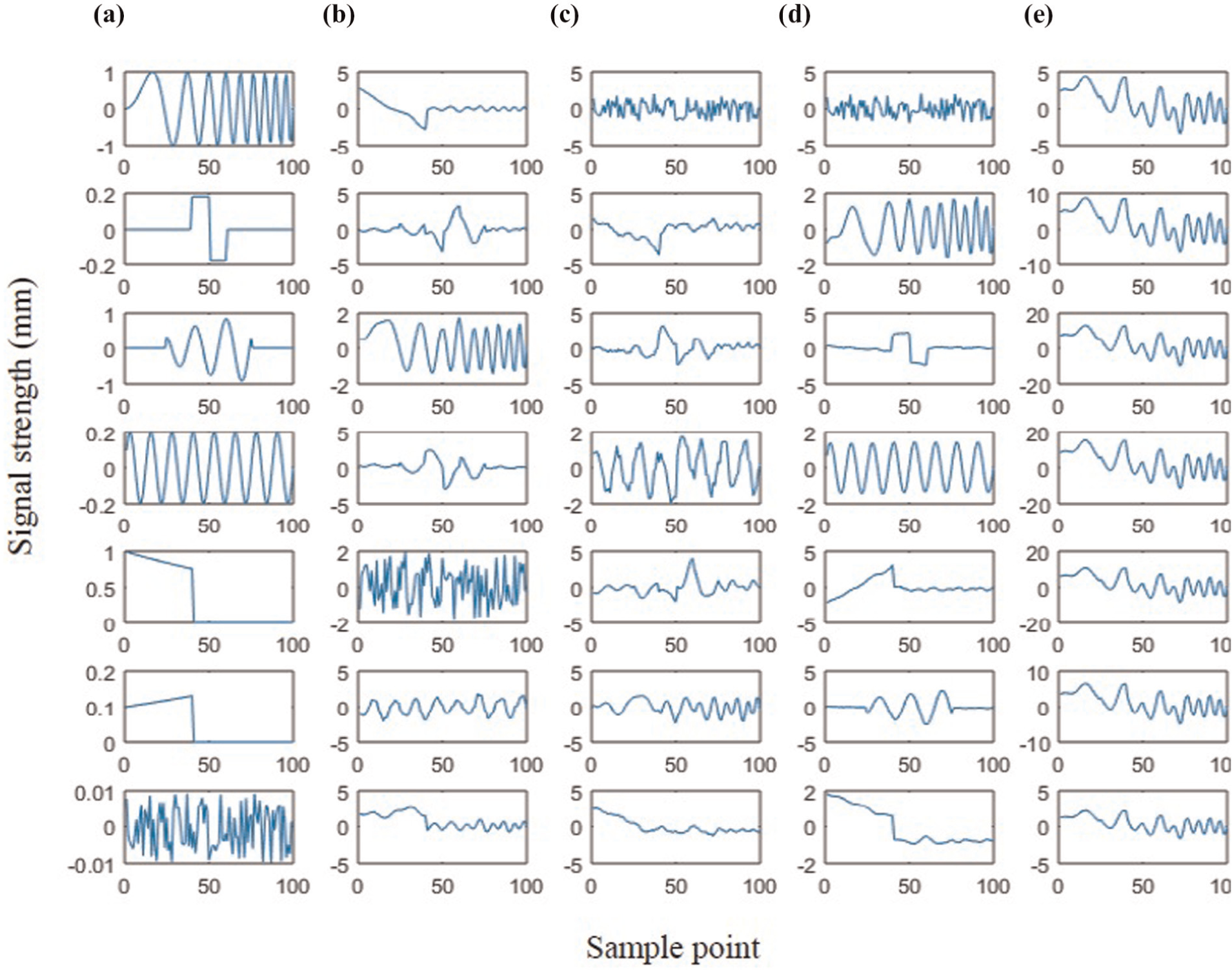
(a) Source signals, (b) separations by FastICA, (c) separations by tensor factorization, (d) separations by ApBSS, and (e) recovery signals by OMP with ApBSS atoms.

Using the separation results in Figure 2(d) as dictionary atoms, applying OMP recovery algorithm creates the recovery signals as shown in Figure 2(e). The recovery signals agree with the observation signals in Figure 1(c). The applicability of the ApBSS algorithm for atoms extraction is found to be superior.

Figure 3 plots the representation coefficients of the observation signals by the extracted atoms. The number of nonzero columns equals the number of observation signals. This kind of sparsest representations illustrates that ApBSS is a powerful algorithm for dictionary building. In addition, the extracted atoms by ApBSS are mutually independent and with zero means, and therefore they would be valuable as orthonormal bases to develop an optimal sparse representation for arbitrary independent signals.

Figure 3.

Representation coefficients of the observation signals using adaptive atoms extracted by ApBSS.

Dictionary representation by extending K-SVD

The step of dictionary representation is performed by the extending K-SVD method.²⁶ The dictionary D is built by shifting a family F of patterns f: $F = (f_{k})_{1 \leq k \leq K}$ . The representation problem of an observation signal y on D can be expressed that minimizes the approximation error under a sparsity constraint

\begin{array}{l} \min_{{‖ x ‖}_{0} \leq K} {‖ y - \sum_{l} \sum_{τ} x_{l, τ} f_{l} (t - τ) ‖}_{2}^{2} \\ = \min_{{‖ x ‖}_{0} \leq K} {‖ y - \sum_{l} \sum_{τ} x_{l, τ} T_{τ} f_{l} ‖}_{2}^{2} \end{array}

(5)

where K is the maximum number of atoms allowed, $T_{τ}$ is the shift operator that takes a pattern f and returns an atom that is null everywhere except for a copy of f that starts at instant $τ$ . In this article, we only considered integer shifts $τ$ .

The representation patterns are updated to minimize the error according to the given supports $σ_{l} = {τ | x_{l, τ} \neq 0}$ . For a given pattern $f_{j}$ , defining ${\hat{y}}_{j} = r + \sum_{τ} x_{j, τ} T_{τ} f_{j}$ the observation signal without the contributions of the other patterns $f_{l}$ where $l \neq j$ ; r is the residual. The best update pattern is given by

(f_{j}, {x_{j}}^{opt}) = argmi n ‖_{f_{2} = 1} {‖ {\hat{y}}_{j} - \sum_{τ \in σ_{j}} x_{τ} T_{τ} f_{j} ‖_{2}}^{2}

(6)

As the shift operators $T_{τ}$ are unitary, therefore

\forall f_{j}, {‖ {\hat{y}}_{j} - \sum_{τ \in σ_{j}} x_{τ} T_{τ} f_{j} ‖_{2}}^{2} = \sum_{τ \in σ_{j}} {‖ {T_{τ}}^{*} {\hat{y}}_{j} - x_{τ} f_{j} ‖_{2}}^{2} + c o n s t

(7)

where ${T_{τ}}^{*}$ is the adjoint of $T_{τ}$ , that is, the operator such that $\forall f, \forall y, < T_{τ} f, y > = < f, {T_{τ}}^{*} y >$ .

Fixing the atoms $f_{j}$ , the minimum of expression (7) is a simple weighted mean

x_{τ} \leftarrow \sum_{τ \in σ_{j}} f_{j} {T_{τ}}^{*} {\hat{y}}_{j} = (\sum_{τ \in σ_{j}} {f_{j}}^{2}) x_{τ} + \sum_{τ \in σ_{j}} f_{j} {T_{τ}}^{*} r, x_{τ} \leftarrow \frac{x_{τ}}{{‖ x_{τ} ‖}_{2}}

(8)

Procedure of the proposed method

The steps for the proposed dictionary learning method are the following:

• Whiten the input signals y

• Compute the eigenvector of

B^{- 1} C

, obtain the separation matrix W

•

f = Wy

, initialize

(f_{k})_{1 \leq k \leq K}

• While the algorithm has not converged do

• for

j = 1

to K do

• initialize

r_{0} = y_{j}

\forall k, \forall τ, x_{k, τ, 0} = 0

• for

i = 1

to K do

•

(k_{i}, τ_{i}) = argma x_{(k, τ)} < r_{i - 1}, T_{τ} f_{k} >

•

δ_{i} = < r_{i - 1}, T_{τ} f_{k} >

x_{k_{i}, τ_{i}, i} = x_{k_{i}, τ_{i}, i - 1} + δ_{i}

•

\forall (k, τ) \neq (k_{i}, τ_{i}), x_{k, τ, i} = x_{k, τ, i - 1}

•

r_{i} = r_{i - 1} - δ_{i} T_{τ_{i}} f_{k_{i}}

• end for

•

x_{τ} \leftarrow \sum_{τ \in σ_{j}} f_{j} {T_{τ}}^{*} {\hat{y}}_{j} = (\sum_{τ \in σ_{j}} {f_{j}}^{2}) x_{τ} + \sum_{τ \in σ_{j}} f_{j} {T_{τ}}^{*} r

•

x_{τ} \leftarrow \frac{x_{τ}}{{‖ x_{τ} ‖}_{2}}

• end for

• end while

Wheel condition monitoring

The procedure of the proposed method for railway wheel condition monitoring is illustrated in Figure 4.

Figure 4.

Procedure of dictionary learning on blind source basis for wheel condition monitoring.

After the data acquisition from the front wheel and the rear wheel, the centrobaric spectrum is calculated as follows

FC = \frac{\sum_{i = 1}^{N} ω_{i} S_{i}}{\sum_{i = 1}^{N} S_{i}}

(9)

where $ω_{i}$ is the frequency value of ith PSD component and $S_{i}$ is the power spectral density value of ith PSD component.

Corresponding to different wear conditions, the wheel has different vibration signatures that largely affect the centrobaric spectrum. Therefore, FC is used as a real-time indicator to reflect the wheel condition. When the centrobaric spectrums $F C_{1}$ of the front wheel and $F C_{2}$ of the rear wheel are different, the new dictionary learning method is applied to recognize the possible wheel defect.

The experiment of wheel condition monitoring is conducted using a JD-1 wheel/rail simulation facility, as shown in Figure 5(a).

Figure 5.

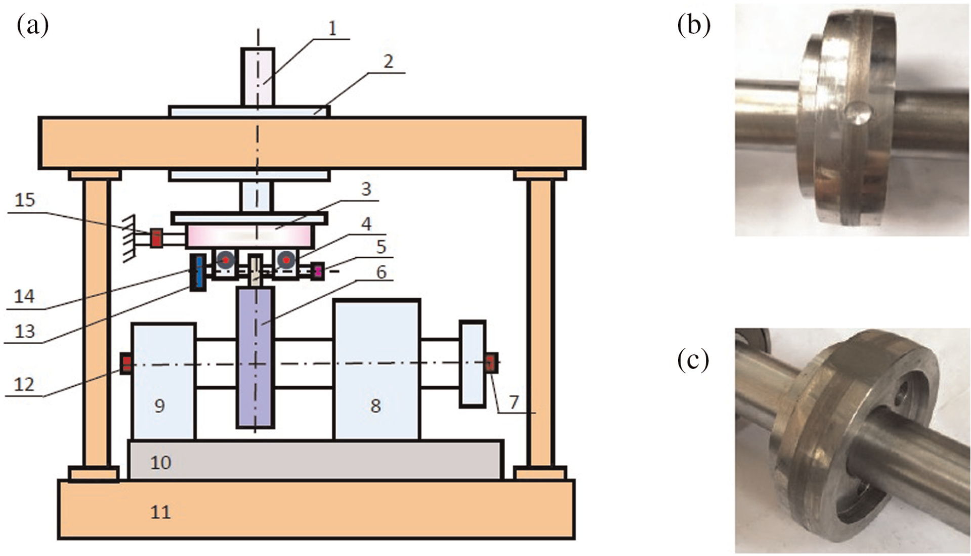
(a) JD-1 wheel/rail simulation facility, (b) wheel flat spot, and (c) wheel tread indentation.

The apparatus is composed of a small roller that serves as the wheel and a large roller that serves as the rail. Two defects are made on the wheel roller: a flat spot shown in Figure 5(b) and a tread indentation shown in Figure 5(c). They are machined 180° from each other. Motor speed imposed on the rollers can be controlled accurately. Two three-dimensional (3D) accelerometers are used to measure the vibration signals. The sampling frequency is 10 kHz.

The wheel roller rotates at a speed of 56 r/min (200 km/h). The longitudinal vibration signals $xs z_{1}$ and $xs z_{2}$ , vertical vibration signal $xs c_{1}$ and $xs c_{2}$ , and transverse vibration signal $xs h_{1}$ and $xs h_{2}$ are presented in Figure 6.

Figure 6.

Vibration observation signals of the wheel roller with two defects.

By the proposed method, the sparse feature columns containing wheel defect information separated by ApBSS are used to build dictionary. The atoms adaptively learned are shown in Figure 7. Atoms a1, a2, and a3 indicate the vertical, longitudinal, and transverse impact responses of the flat spot, respectively. Atoms b1, b2, and b3 are the corresponding responses of the tread indentation impact.

Figure 7.

Wheel defect atoms extracted by the proposed method.

Take the vertical wheel–rail impact response due to the wheel flat to analyze the theoretical correctness of the defect atoms extracted by the proposed method. For descriptions of wheel–rail contact dynamic procedure, given a wheel with a theoretical flat of length l and depth d, as shown in Figure 8.

Figure 8.

Rolling wheel with a theoretical flat and wheel–rail contact force due to the flat.

Michaël and Steenbergen²⁷ qualitatively derived the vertical contact force $F (t)$ between the wheel and the foundation as equation (10), which is plotted with red dotted line in Figure 8

\begin{array}{l} F (t) = \frac{- m V^{2} R^{2}}{\sqrt{{(R^{2} - V^{2} t^{2})}^{3}}} H (- t + \frac{l}{2 V}) \\ + δ (t - \frac{l}{2 V}) - \frac{- m V^{2} R^{2}}{\sqrt{{(R^{2} - {(V t - l)}^{2})}^{3}}} \\ [H (t - \frac{l}{2 V}) - H (t - \frac{l}{V})] \end{array}

(10)

where $H (\cdot)$ represents the Heaviside function; V is the train speed.

The flat response signal extracted by ApBSS is shown in the upper graph with blue line in Figure 9, which is excellently correspondent to the theoretical derived function as plotted in Figure 9 with red dotted line, especially when the elasticity of track and wheel is taken into account.

Figure 9.

Flat response signal and its Choi–Williams time–frequency distribution.

The time–frequency representation of the wheel flat is analyzed by Choi–Williams time–frequency distribution, as shown in the bottom graph in Figure 9. Choi–Williams time–frequency distribution is a kind of Cohen’s class of distributions defined as follows²⁸

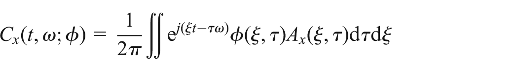
C_{x} (t, ω; ϕ) = \frac{1}{2 π} \int \int e^{j (ξ t - τ ω)} ϕ (ξ, τ) A_{x} (ξ, τ) d τ d ξ

where $A_{x} (ξ, τ)$ is the ambiguity function of $x (t)$ ; kernel function $ϕ (ξ, τ) = \exp ((- ξ^{2} τ^{2}) / (σ)), σ > 0$ , where $σ$ is a scaling parameter.

Experimental measurement and theoretical analysis are validated mutually, which indicates that the wheel–rail interaction due to wheel wear extracted by the proposed method accurately reflects the wheel wear feature. The proposed method can adaptively learn and accurately identify the wheel defects.

Conclusion

Online recognition of wheel wear is crucial for effective maintenance and is a challenging area of railway safety operation. The observation signal of wheel–rail interaction due to wheel wear is the mixture of the wear impact response signal and the common wheel–rail contact signal. Because slight wear signals are often concealed by severe wheel–rail contact signals in time domain and their spectrums overlap in frequency domain, the conventional time–frequency analysis and frequency filtering technique often cannot accurately extract the early wheel wear from the wheel–rail interaction observation signals.

A new dictionary learning approach for wheel condition monitoring is proposed. Flexible decompositions are particularly important for representing signal components whose locations in time and frequency vary widely. In order to overcome the deficiency of the existing dictionary learning methods, this article presents the new dictionary learning method based on ApBSS and extending K-SVD and applies it to wheel defect detection. Numerical simulations confirm the effectiveness of the developed method. An experiment of wheel condition monitoring is conducted using a JD-1 wheel/rail simulation facility. By adapting the atoms to the input, the proposed method yields sparse representations for arbitrary independent signals as well as capture detail defect information from the observation signals. Data calculating and theoretical analysis of wheel–rail contact dynamic show that the proposed method can adaptively learn and accurately identify the wheel defects and verify the performance of the proposed method.

Footnotes

Academic Editor: Dong Wang

Declaration of conflicting interests

The author(s) declared no potential conflicts of interest with respect to the research, authorship, and/or publication of this article.

Funding

The author(s) disclosed receipt of the following financial support for the research, authorship, and/or publication of this article: This research was supported by grants from the National Natural Science Foundation of China (no. 51205323).

References

Cigada

Manzoni

Vanali

Geometry effects on the vibro-acoustic behavior of railway resilient wheels. J Vib Control 2011; 17: 1761–1778.

Belotti

Crenna

Michelini

. Wheel-flat diagnostic tool via wavelet transform. Mech Syst Signal Pr 2006; 20: 1953–1966.

Thakkar

Steel

Reuben

RL.

Rail-wheel interaction monitoring using acoustic emission: a laboratory study of normal rolling signals with natural rail defects. Mech Syst Signal Pr 2010; 24: 256–267.

Bernal

Martinod

Betancur

GR.

Partial-profilogram reconstruction method to measure the geometric parameters of wheels in dynamic condition. Vehicle Syst Dyn 2016; 54: 606–616.

Zhang

Gao

Liu

. A new real-time signal processing approach of frequency-varying machinery. J Vib Control. Epub ahead of print 5 January 2017. DOI: 10.1177/1077546316687923.

Liang

Iwnicki

Zhao

. Railway wheel-flat and rail surface defect modelling and analysis by time-frequency techniques. Vehicle Syst Dyn 2013; 51: 1403–1421.

Tosic

Frossard

Dictionary learning. IEEE Signal Proc Mag 2011; 28: 27–38.

Mostafa

Massoud

Christian

Learning overcomplete dictionaries based on atom-by-atom updating. IEEE T Signal Proces 2014; 62: 883–891.

Engan

Aase

Husoy

JH.

Method of optimal directions for frame design. Int Conf Acoust Spee 1999; 5: 2443–2446.

10.

Aharon

Elad

Bruckstein

K-SVD: an algorithm for designing overcomplete dictionaries for sparse representation. IEEE T Signal Proces 2006; 54: 4311–4322.

11.

Tropp

Wright

SJ.

Computational methods for sparse solution of linear inverse problems. Proc IEEE 2010; 98: 948–958.

12.

Pati

Rezaiifar

Krishnaprasad

PS.

Orthogonal matching pursuit: recursive function approximation with applications to wavelet decomposition. In: Proceedings of the twenty-seventh Asilomar conference on signals, systems and computers, Pacific Grove, CA, 1–3 November 1993, pp.40–44. New York: IEEE.

13.

Needell

Tropp

JA.

CoSaMP: iterative signal recovery from in-complete and inaccurate samples. Commun ACM 2009; 26: 301–321.

14.

Dai

Milenkovic

Subspace pursuit for compressive sensing signal reconstruction. IEEE T Inform Theory 2009; 55: 2230–2249.

15.

Daubechies

Defrise

DeMol

An iterative thresholding algorithm for linear inverse problems with a sparsity constraint. Commun Pur Appl Math 2004; 57: 1413–1457.

16.

Mohimani

BabaieZadeh

Jutten

A fast approach for overcomplete sparse decomposition based on smoothed ℓ⁰ norm. IEEE T Signal Proces 2009; 57: 289–301.

17.

Kim

Koh

Lustig

. An interior point method for large-scale-regularized least squares. IEEE J STSP 2007; 1: 606–617.

18.

Kreutz

Murray

Rao

. Dictionary learning algorithms for sparse representation. Neural Comput 2003; 15: 349–396.

19.

Davis

Mallat

Avellaneda

Adaptive greedy approximations. Constr Approx 1997; 13: 57–98.

20.

Bechler

Wojtaszczyk

Error estimates for orthogonal matching pursuit and random dictionaries. Constr Approx 2011; 33: 273–288.

21.

Tse

Zhang

Wang

XJ.

Blind source separation and blind equalization algorithms for mechanical signal separation and identification. J Vib Control 2006; 12: 395–423.

22.

Zhang

Gao

A new method for blind separation of nonstationary sources. J Vib Control 2016; 22: 2873–2884.

23.

Jeremy

Jerome

Anthony

. Sparse and non-negative BSS for noisy data. IEEE T Signal Proces 2013; 61: 5620–5632.

24.

Beckmann

Smith

SM.

Probabilistic independent component analysis for functional magnetic resonance imaging. IEEE T Med Imaging 2004; 23: 137–152.

25.

Yongchao

Satish

Output-only modal identification with limited sensors using sparse component analysis. J Sound Vib 2013; 332: 4741–4765.

26.

Mailhé

Lesage

Gribonval

. Shift-invariant dictionary learning for sparse representations: extending K-SVD. In: Proceedings of the 16th European signal processing conference, Lausanne, Switzerland, 25–29 August 2008, pp.1–5. New York: IEEE.

27.

Michaël

Steenbergen

The role of the contact geometry in wheel-rail impact due to wheel flats. Vehicle Syst Dyn 2007; 45: 1097–1116.

28.

Antonia

Faye

GB.

Generalization of the Choi-Williams distribution and the Butterworth distribution for time-frequency analysis. IEEE T Signal Proces 1993; 41: 463–472.

A novel dictionary learning approach based on blind source separation basis and its application

Abstract

Keywords

Introduction

Classical dictionary learning method

A new method of dictionary learning in blind source basis

Atoms extraction by ApBSS

Dictionary representation by extending K-SVD

Procedure of the proposed method

Wheel condition monitoring

Conclusion

Footnotes

Declaration of conflicting interests

Funding

References