On the numerical solution of a singular second-order thermoelastic system

Abstract

In this article, we study an initial boundary value problem for a coupled system of thermoelasticity. Some existence and uniqueness results are given. The homotopy analysis method is employed to obtain numerical schemes for solving the posed problem. The efficiency of the derived methods is illustrated through several examples with graphical representations.

Introduction

Linear thermoelastic systems have been studied by many researchers. For example, results dealing with existence and asymptotic behaviors were studied in some literature;^1–6 controllability in Bardos et al. ⁷ and Zuazua; ⁸ propagation of singularities in Hrusa and Messaoudi ⁹ and Racke and Wang; ¹⁰ and regularity, decay, and blow up of solutions in Messaoudi ¹¹ and Rivera and Racke. ¹² In this article, we are interested in studying the numerical solutions of an initial boundary value problem with Dirichlet conditions for a system of linear thermoelasticity with a coupling parameter. We first give some existence and uniqueness results. Then, we proceed to numerical solutions using the homotopy analysis method (HAM). The precise statement of the given initial boundary value problem is as follows: Let $T>0,$ $\mathrm{\Omega }=(0,1),$ and $I=(0,T)$ , and consider the following coupling system

$$\{\begin{array}{c}{\mathcal{L}}_1(u,v)=u_{\mathrm{tt}}-\frac{a}{x}{(x{u}_x)}_x+\mathrm{bx}{v}_x=f(x,t)\hfill \\ \multicolumn{1}{c}{{\mathcal{L}}_2(u,v)=v_t-\frac{\mu }{x}{(x{v}_x)}_x+\mathrm{bx}{u}_{\mathrm{tx}}=g(x,t)}\end{array}$$

(1)

System (1) describes a model for the symmetric deformation and temperature distribution in the unit disk. When $b=0$ , the system decouples, and we have the wave and the heat equations. The appearance of Bessel operator in the first and second equations in system (1) comes from the fact that Laplace operator can be written in that form when we focus for radial solutions and in this case, the functions $f,g,u_0,u_1$ , and $v_0$ must be radial. In this mathematical model, the functions $u,v,f$ , and g represent the displacement, difference absolute temperature, external force, and the heat supply, respectively, and $a,b,\mu$ are positive constants.

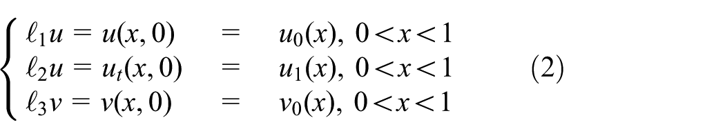
System (1) is associated with the initial conditions

$$\{\begin{array}{ccc}{\ell }_{1}u=u(x,0)\hfill & =\hfill & u_0(x),0<x<1\hfill \\ \multicolumn{1}{c}{{\ell }_{2}u=u_t(x,0)}& =\hfill & u_1(x),0<x<1\hfill \\ \multicolumn{1}{c}{{\ell }_{3}v=v(x,0)}& =\hfill & v_0(x),0<x<1\hfill \end{array}$$

(2)

and the boundary conditions

$$\{\begin{array}{ccc}u(1,t)\hfill & =\hfill & 0,0<t<T\hfill \\ \multicolumn{1}{c}{v(1,t)}& =\hfill & 0,0<t<T\hfill \end{array}$$

(3)

We assume that the data satisfy the compatibility conditions: $u_0(1)=0,u_1(1)=0$ , and $v_0(1)=0$ . Our main concern as mentioned previously is to study numerical solutions of problems (1)–(3). For this purpose, we apply the HAM to derive numerical solutions of system (1) along with the boundary and initial conditions given in equations (2) and (3).

In fact, we obtain a family of series solutions of the given coupled thermoelasticity system by using the initial conditions (partial t-solution). By this method, we could control the convergence region and the rate of the series solutions.

The HAM was initially proposed by Liao ¹³ in 1992 (see also Liao^14–16). Since then, it has been employed to solve many types of ordinary and partial differential equations characterizing many problems in applied sciences and engineering (see Bataineh et al. ¹⁷ and Hayat et al. ¹⁸ and the references therein). A modification of the HAM to solve systems of partial differential equations is presented in Bataineh et al. ¹⁷

The rest of the article is organized as follows: in section “Some existence and unique results,” we give some existence and uniqueness results. In section “Application of the HAM,” we apply the method and give some applications by treating several examples to test the efficiency of the method.

Some existence and uniqueness results

We first introduce some function spaces needed in the sequel. Let $L_{\rho }^2(\mathrm{\Omega })$ be the weighted $L^2(\mathrm{\Omega })$ Hilbert space equipped with the inner product $(u,v{)}_{L_{\rho }^2(Q)}={\int }_Q\mathrm{xuvdxdt}.$ The space $H_{2,\rho }^1(\mathrm{\Omega })$ denotes the Hilbert space obtained by completing $C^1(\mathrm{\Omega })$ with respect to the norm

$$\Vert u{\Vert }_{H_{2,\rho }^1(\mathrm{\Omega })}^2=\Vert u{\Vert }_{L_{\rho }^2(\mathrm{\Omega })}^2+\Vert u_x{\Vert }_{L_{\rho }^2(\mathrm{\Omega })}^2$$

and with associated inner product

$$(u,v{)}_{H_{2,\rho }^1(\mathrm{\Omega })}=(u,v{)}_{L_{\rho }^2(\mathrm{\Omega })}+(u_x,v_x{)}_{L_{\rho }^2(\mathrm{\Omega })}$$

The set $C(\overline{I},Y)$ with $\overline{I}=[0,T],$ is the space of continuous mappings from $\overline{I}$ onto a Banach space $Y.$

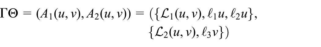
Our problems (1)–(3) can be considered as the problem of solving the equation $\mathrm{\Gamma }\mathrm{\Theta }=\mathcal{F},$ where $\mathrm{\Theta }=(u,v)$ and $\mathcal{F}=({\mathcal{F}}_1,{\mathcal{F}}_2)=(\{f,u_0,u_1\},\{g,v_0\})$ , and $\mathrm{\Gamma }$ is the operator given by

$$\mathrm{\Gamma }\mathrm{\Theta }=(A_1(u,v),A_2(u,v))=(\{{\mathcal{L}}_1(u,v),{\ell }_{1}u,{\ell }_{2}u\},\{{\mathcal{L}}_2(u,v),{\ell }_{3}v\})$$

where

$$A_1(u,v)=\{{\mathcal{L}}_1(u,v),{\ell }_{1}u,{\ell }_{2}u\},A_2(u,v)=\{{\mathcal{L}}_2(u,v),{\ell }_{3}v\}$$

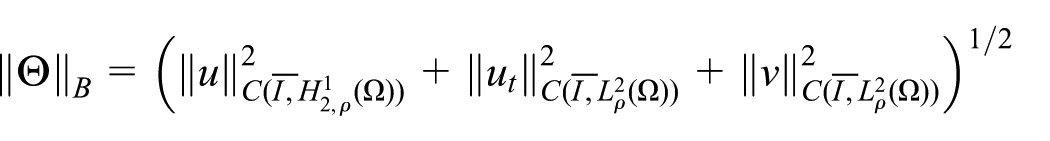
The operator $\mathrm{\Gamma }:B\to H$ is considered as an unbounded operator acting on a Banach space B into a Hilbert space H, and with domain denoted by $D(\mathrm{\Gamma })$ which is the set of functions $\mathrm{\Theta }=(u,v)\in L^2(I,L_{\rho }^2(\mathrm{\Omega }){)}^2$ for which $u_t,$ $v_t,$ $u_{\mathrm{tt}},$ $u_x,$ $v_x,$ $u_{\mathrm{xx}},v_{\mathrm{xx}},u_{\mathrm{tx}},v_{\mathrm{tx}}\in L^2(I,L_{\rho }^2(\mathrm{\Omega }))$ and satisfies the boundary condition $(3).$ The Banach space B is obtained by the closure of $D(\mathrm{\Gamma })$ in the norm

$$\Vert \mathrm{\Theta }{\Vert }_B={(\Vert u{\Vert }_{C(\overline{I,}{H}_{2,\rho }^1(\mathrm{\Omega }))}^2+\Vert u_t{\Vert }_{C(\overline{I,}{L}_{\rho }^2(\mathrm{\Omega }))}^2+\Vert v{\Vert }_{C(\overline{I,}{L}_{\rho }^2(\mathrm{\Omega }))}^2)}^{1/2}$$

where

$$\begin{array}{c}\Vert u{\Vert }_{C(\overline{I,}{H}_{2,\rho }^1(\mathrm{\Omega }))}^2=\underset{0\le \tau \le T}{sup}\Vert u(x,\tau ){\Vert }_{H_{2,\rho }^1(\mathrm{\Omega })}^2\hfill \\ \Vert u_t{\Vert }_{C(\overline{I,}{L}_{\rho }^2(\mathrm{\Omega }))}^2=\underset{0\le \tau \le T}{sup}\Vert u_t(x,\tau ){\Vert }_{L_{\rho }^2(\mathrm{\Omega })}^2\hfill \end{array}$$

and

$$\Vert v{\Vert }_{C(\overline{I,}{L}_{\rho }^2(\mathrm{\Omega }))}^2=\underset{0\le \tau \le T}{sup}\Vert v(x,\tau ){\Vert }_{L_{\rho }^2(\mathrm{\Omega })}^2$$

The set H is the Hilbert space $\{L_{\rho }^2(Q)\times H_{2,\rho }^1(\mathrm{\Omega })\times L_{\rho }^2(\mathrm{\Omega })\}\times \{L_{\rho }^2(Q)\times L_{\rho }^2(\mathrm{\Omega })\}$ consisting of vector-valued functions $\mathcal{F}=({\mathcal{F}}_1,{\mathcal{F}}_2)=(\{f,u_0,u_1\},\{g,v_0\})$ for which the norm

$${\Vert ℱ\Vert }_H={({\Vert f\Vert }_{L^2(I,L_{\rho }^2(\Omega )}^2+{\Vert u_0\Vert }_{H_{2,\rho }^1(\Omega )}^2+{\Vert u_1\Vert }_{L_{\rho }^2(\Omega )}^2+{\Vert g\Vert }_{L^2(I,L_{\rho }^2(\Omega )}^2+{\Vert v_0\Vert }_{L_{\rho }^2(\Omega )}^2)}^{1/2}$$

is finite.

The associated inner product in H is defined by

$$\begin{array}{c}\multicolumn{1}{c}{(\mathcal{F},{\mathcal{F}}^{*}{)}_H=({\mathcal{L}}_1(u,v),w_1{)}_{L_{\rho }^2(Q)}+({\ell }_{1}u,w_3{)}_{H_{\rho }^1(\mathrm{\Omega })}}\\ \multicolumn{1}{c}{+({\ell }_{2}u,w_4{)}_{L_{\rho }^2(\mathrm{\Omega })}+({\mathcal{L}}_2(u,v),w_2{)}_{L_{\rho }^2(Q)}}\\ \multicolumn{1}{c}{+({\ell }_{3}v,w_5{)}_{L_{\rho }^2(\mathrm{\Omega })}}\end{array}$$

where

$${\mathcal{F}}^{*}=(\{w_1,w_3,w_4\},\{w_2,w_5\})$$

We observe that the mappings

$$\begin{array}{c}{\ell }_1:B\ni u\to {\ell }_{1}u=u{|}_{t=0}\in H_{2,\rho }^1(\mathrm{\Omega })\hfill \\ {\ell }_2:B\ni u\to {\ell }_{2}u=u_t{|}_{t=0}\in L_{\rho }^2(\mathrm{\Omega })\hfill \\ {\ell }_3:B\ni v\to {\ell }_{3}v=v{|}_{t=0}\in L_{\rho }^2(\mathrm{\Omega })\hfill \end{array}$$

are defined and continuous on the Banach space $B,$ because the elements u are continuous functions on $[0,T]$ with values in $H_{2,\rho }^1(\mathrm{\Omega })$ , and have derivatives $u_t$ continuous on $[0,T]$ with values in $L_{\rho }^2(\mathrm{\Omega })$ , and the elements v are continuous functions on $[0,T]$ with values in $L_{\rho }^2(\mathrm{\Omega })$ .

Before proceeding to numerical solutions of the given problems $(1)-(3)$ , we may state and prove in a short way some existence and uniqueness results. For more details, see literature.^19–21 We first establish a priori estimate for the solution from which the uniqueness of the solution follows. Then, based on the density of the range of the operator generated by the problem in consideration, we prove the existence of the solution of problems $(1)-(3)$ .

Theorem 1

There exists a positive constant C not depending on $\mathrm{\Theta }=(u,v),$ such that

$$\Vert \mathrm{\Theta }{\Vert }_B\le C\Vert \mathrm{\Gamma }\mathrm{\Theta }{\Vert }_H$$

(4)

holds for all functions $\mathrm{\Theta }=(u,v)\in D(\mathrm{\Gamma })$ .

Proof

We multiply the first equation in system $(1)$ by the operator $N_1=x{u}_t$ and the second equation by $N_2=\mathrm{xv},$ then taking into account the boundary and initial conditions, we evaluate the integrals

$$\begin{array}{c}\multicolumn{1}{c}{{\int }_{Q^{\tau }}x{u}_t\mathrm{udxdt};-a{\int }_{Q^{\tau }}(x{u}_x{)}_x{u}_t\mathrm{dxdt};{\int }_{Q^{\tau }}\mathrm{xv}{v}_t\mathrm{dxdt};}\\ \multicolumn{1}{c}{-\mu {\int }_{Q^{\tau }}(x{v}_x{)}_x\mathrm{vdxdt};b{\int }_{Q^{\tau }}{x}^2{u}_{\mathrm{xt}}\mathrm{vdxdt};b{\int }_{Q^{\tau }}{x}^2{u}_t{v}_x\mathrm{dxdt}}\end{array}$$

over the domain $Q^{\tau }=(0,\tau )\times \mathrm{\Omega }$ to obtain

$$\begin{array}{l}a{\displaystyle {\int }_{\Omega }x}{u}_x^2(x,\tau )dx+{\displaystyle {\int }_{\Omega }x}{u}_t^2(x,\tau )dx+{\displaystyle {\int }_{\Omega }x}{v}^2(x,\tau )dx+2\mu {\displaystyle {\int }_{Q^{\tau }}x}{v}_x^{2}dxdt\\ ={\displaystyle {\int }_{\Omega }x}{u}_1^{2}dx+a{\displaystyle {\int }_{\Omega }x}{(\frac{\partial u_0}{\partial x})}^{2}dx+{\displaystyle {\int }_{\Omega }x}{v}_0^{2}dx\\ +2b{\displaystyle {\int }_{Q^{\tau }}x}{u}_{t}vdxdt+2{\displaystyle {\int }_{Q^{\tau }}x}{u}_{t}fdxdt+2{\displaystyle {\int }_{Q^{\tau }}x}vgdxdt\\ \le {\displaystyle {\int }_{\Omega }x}{u}_1^{2}dx+a{\displaystyle {\int }_{\Omega }x}{(\frac{\partial u_0}{\partial x})}^{2}dx+{\displaystyle {\int }_{\Omega }x}{v}_0^{2}dx\\ +b^2{\displaystyle {\int }_{Q^{\tau }}x}{u}_t^{2}dxdt+{\displaystyle {\int }_{Q^{\tau }}x}{v}^{2}dxdt+{\displaystyle {\int }_{Q^{\tau }}x}{f}^{2}dxdt+{\displaystyle {\int }_{Q^{\tau }}x}{g}^{2}dxdt\end{array}$$

(5)

The following elementary inequality is essential in our proof

$${\displaystyle {\int }_{\Omega }x}{u}^2(x,\tau )dx\le {\displaystyle {\int }_{Q^{\tau }}x}{u}^{2}dxdt+{\displaystyle {\int }_{Q^{\tau }}x}{u}_t^{2}dxdt+{\displaystyle {\int }_{\Omega }x}{u}_0^2(x)dx$$

(6)

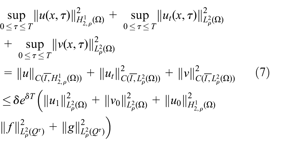
By adding side to side the inequalities $(5)$ and $(6)$ , using Cauchy- $\epsilon$ inequality, discarding the positive fourth term on the left-hand side of $(5)$ , applying Gronwall’s lemma in Garding, ²² and then passing to the supremum with respect to $\tau$ over $[0,T]$ in the resulted inequality, we obtain in terms of norms

$$\begin{array}{c}\multicolumn{1}{c}{\underset{0\le \tau \le T}{sup}\Vert u(x,\tau ){\Vert }_{H_{2,\rho }^1(\mathrm{\Omega })}^2+\underset{0\le \tau \le T}{sup}\Vert u_t(x,\tau ){\Vert }_{L_{\rho }^2(\mathrm{\Omega })}^2}\\ \multicolumn{1}{c}{+\underset{0\le \tau \le T}{sup}\Vert v(x,\tau ){\Vert }_{L_{\rho }^2(\mathrm{\Omega })}^2}\\ \multicolumn{1}{c}{={\Vert u\Vert }_{C(\overline{I,}{H}_{2,\rho }^1(\mathrm{\Omega }))}+\Vert u_t{\Vert }_{C(\overline{I,}{L}_{\rho }^2(\mathrm{\Omega }))}^2+\Vert v{\Vert }_{C(\overline{I,}{L}_{\rho }^2(\mathrm{\Omega }))}^2}\\ \multicolumn{1}{c}{\le \delta e^{\delta T}(\Vert u_1{\Vert }_{L_{\rho }^2(\mathrm{\Omega })}^2+\Vert v_0{\Vert }_{L_{\rho }^2(\mathrm{\Omega })}^2+\Vert u_0{\Vert }_{H_{2,\rho }^1(\mathrm{\Omega })}^2}\\ \multicolumn{1}{c}{\Vert f{\Vert }_{L_{\rho }^2(Q^{\tau })}^2+\Vert g{\Vert }_{L_{\rho }^2(Q^{\tau })}^2)}\end{array}$$

(7)

where $\delta =\frac{max(1,a,b^2+1)}{min(a,2)}.$ Then, inequality $(4)$ follows with $C={\delta }^{1/2}{e}^{\delta T/2}.$ Let $\mathrm{Im}\mathrm{\Gamma }$ denote the range or the image of the operator $\mathrm{\Gamma },$ since we have no information about $\mathrm{Im}\mathrm{\Gamma }$ except that $\mathrm{Im}\mathrm{\Gamma }\subset H,$ hence, we have to make an extension to $\mathrm{\Gamma }$ denoted by $\overline{\mathrm{\Gamma }},$ so that we have

$$\Vert \mathrm{\Theta }{\Vert }_B\le C\Vert \overline{\mathrm{\Gamma }}\mathrm{\Theta }{\Vert }_H$$

(8)

and $\mathrm{Im}\overline{\mathrm{\Gamma }}=H.$ It can be shown in a very classical way that the operator $\mathrm{\Gamma }:B\to H$ has a closure $\overline{\mathrm{\Gamma }}.$

Definition 1

The solution of the operator equation $\overline{\mathrm{\Gamma }}\mathrm{\Theta }=\mathcal{F}$ is called a strong solution of the posed problems $(1)-(3)$ .

In view of inequality $(8)$ , we deduce that a strong solution of problems $(1)-(3)$ is unique and depends continuously on the elements ${\mathcal{F}}_1=\{f,u_0,u_1\}$ and ${\mathcal{F}}_2=\{g,{\theta }_0\}$ , and that the image of $\overline{\mathrm{\Gamma }}$ is closed in H and coincides with the closure of the image of $\mathrm{\Gamma }$ . That is, $\mathrm{Im}\overline{\mathrm{\Gamma }}=\overline{\mathrm{Im}\mathrm{\Gamma }}.$

Theorem 2

Problems $(1)-(3)$ admit a unique strong solution satisfying

$$u\in C(\overline{I,}{H}_{2,\rho }^1(\mathrm{\Omega })),u_t\in C(\overline{I,}{L}_{\rho }^2(\mathrm{\Omega })),v\in C(\overline{I,}{L}_{\rho }^2(\mathrm{\Omega }))$$

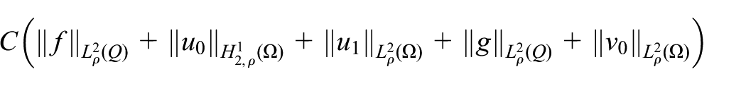
and the norms $\Vert u{\Vert }_{C(\overline{I,}{H}_{2,\rho }^1(\mathrm{\Omega }))},\Vert u_t{\Vert }_{C(\overline{I,}{L}_{\rho }^2(\mathrm{\Omega }))},\Vert v{\Vert }_{C(\overline{I,}{L}_{\rho }^2(\mathrm{\Omega }))}$ are bounded above by

$$C({\Vert f\Vert }_{L_{\rho }^2(Q)}+{\Vert u_0\Vert }_{H_{2,\rho }^1(\Omega )}+{\Vert u_1\Vert }_{L_{\rho }^2(\Omega )}+{\Vert g\Vert }_{L_{\rho }^2(Q)}+{\Vert v_0\Vert }_{L_{\rho }^2(\Omega )})$$

Proof

To prove the existence of the solution, it is sufficient to show that $\overline{\mathrm{Im}\mathrm{\Gamma }}=H$ ( $\mathrm{\Gamma }$ is surjective). This means that we have to show that the orthogonal complement of the image of $\mathrm{\Gamma }$ reduces to zero, that is, $\{\mathrm{Im}\mathrm{\Gamma }{\}}^{\perp }=\{0\}$ . In fact, this is equivalent to $(\mathcal{F},{\mathcal{F}}^{*}{)}_H=0$ . Moreover, since H is a Hilbert space, the equality $\overline{\mathrm{Im}\mathrm{\Gamma }}=H$ holds if and only if from the identity

$$\begin{array}{l}{(ℱ,{ℱ}^{\ast })}_H={({ℒ}_1(u,v),w_1)}_{L_{\rho }^2(Q)}+{({\ell }_{1}u,w_3)}_{H_{\rho }^1(\Omega )}+{({\ell }_{2}u,w_4)}_{L_{\rho }^2(\Omega )}\\ +{({ℒ}_2(u,v),w_2)}_{L_{\rho }^2(Q)}+{({\ell }_{3}v,w_5)}_{L_{\rho }^2(\Omega )}=0\end{array}$$

(9)

where $\mathrm{\Theta }=(u,v)$ runs over B, while ${\mathcal{F}}^{*}=({\mathcal{F}}_1^{*},{\mathcal{F}}_2^{*})=(\{w_1,w_3,w_4\},\{w_2,w_5\})\in H,$ and there follows that ${\mathcal{F}}^{*}=0.$ For the moment, we assume that the following theorem is valid

Theorem 3

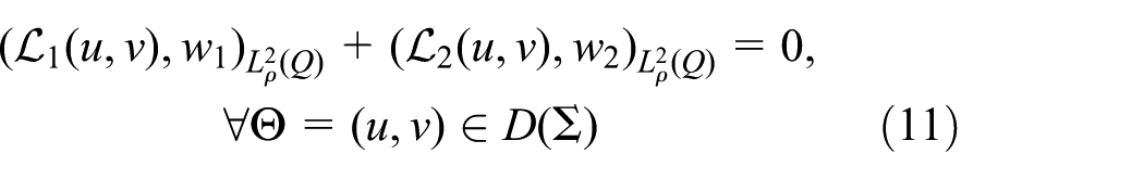
If, for some function $\omega =(w_1,w_2)\in (L_{\rho }^2(Q){)}^2$ and for all elements $\mathrm{\Theta }\in D_0(\mathrm{\Gamma })=\{\mathrm{\Theta }/\mathrm{\Theta }\in D(\mathrm{\Gamma }):{\ell }_{1}u={\ell }_{2}u={\ell }_{3}v=0\},$ we have

$$({\mathcal{L}}_1(u,v),w_1{)}_{L_{\rho }^2(Q)}+({\mathcal{L}}_2(u,v),w_2{)}_{L_{\rho }^2(Q)}=0$$

(10)

then, $\omega$ vanishes almost everywhere in $Q$ .

Particularly by putting $\mathrm{\Theta }\in D_0(\mathrm{\Gamma })$ in (9), we obtain

$$({\mathcal{L}}_1(u,v),w_1{)}_{L_{\rho }^2(Q)}+({\mathcal{L}}_2(u,v),w_2{)}_{L_{\rho }^2(Q)}=0,\forall \mathrm{\Theta }=(u,v)\in D(\Sigma )$$

(11)

Then, we conclude by theorem 3 that $\omega =(w_1,w_2)=0.$ Consequently, for all $\mathrm{\Theta }\in B,$ we have

$$({\ell }_{1}u,w_3{)}_{H_{\rho }^1(\mathrm{\Omega })}+({\ell }_{2}u,w_4{)}_{L_{\rho }^2(\mathrm{\Omega })}+({\ell }_{3}v,w_5{)}_{L_{\rho }^2(\mathrm{\Omega })}=0$$

(12)

Since the three terms in $(12)$ vanish independently, and since the images $\mathrm{Im}({\ell }_1),$ $\mathrm{Im}({\ell }_2)$ , and $\mathrm{Im}({\ell }_3)$ of the operators ${\ell }_1,{\ell }_2$ , and ${\ell }_3$ are everywhere dense in the spaces $H_{2,\rho }^1(\mathrm{\Omega }),$ $L_{\rho }^2(\mathrm{\Omega }),$ and $L_{\rho }^2(\mathrm{\Omega })$ , respectively, then $(12)$ implies that $w_3=0,w_4=0,w_5=0.$ Hence, $\overline{\mathrm{Im}\mathrm{\Gamma }}=H.$

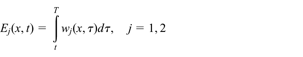
In order to conclude our considerations, we prove theorem 3.

First, define the functions $E_j$ by the relation

$$E_j(x,t)=\underset{t}{\overset{T}{\int }}{w}_j(x,\tau )d\tau ,j=1,2$$

Let $(x{u}_{\mathrm{tt}},x{v}_t)$ be the solution of the system

$$\{\begin{array}{c}x{u}_{\mathrm{tt}}=E_1(x,t)\hfill \\ \multicolumn{1}{c}{x{v}_t=E_2(x,t)}\end{array}$$

(13)

and let

$$\mathrm{\Theta }(x,t)=(\underset{s}{\overset{t}{\int }}(\tau -t)u_{\tau \tau }d\tau ,\underset{s}{\overset{t}{\int }}{v}_{\tau }d\tau ),\mathrm{for}s\le t\le T\mathrm{and}(0,0)\mathrm{for}0\le t\le s$$

(14)

We have

$$w_1=-x{u}_{\mathrm{ttt}},w_2=-x{v}_{\mathrm{tt}}$$

(15)

Replacing the functions $w_1$ and $w_2$ , given by $(15)$ , in the relation $(10)$ , we obtain

$$\begin{array}{c}\multicolumn{1}{c}{-{(u_{\mathrm{tt}},u_{\mathrm{ttt}})}_{L_{\rho }^2(Q)}+a{(u_{\mathrm{ttt}},(x{u}_x{)}_x)}_{L^2(Q)}-b{(x{v}_x,u_{\mathrm{ttt}})}_{L_{\rho }^2(Q)}}\\ \multicolumn{1}{c}{-{(v_t,v_{\mathrm{tt}})}_{L_{\rho }^2(Q)}+k{(v_{\mathrm{tt}},(x{v}_x{)}_x)}_{L^2(Q)}-b{(x{v}_{\mathrm{tt}},u_{\mathrm{tx}})}_{L_{\rho }^2(Q)}=0}\end{array}$$

(16)

In the presence of relations $(13)$ and $(14)$ , and the boundary conditions (3), equation (16) becomes

$$\begin{array}{c}\multicolumn{1}{c}{+\frac{1}{2}\Vert v_t(x,s){\Vert }_{L_{\rho }^2(\mathrm{\Omega })}^2+\frac{1}{2}\Vert u_{\mathrm{tt}}(x,s){\Vert }_{L_{\rho }^2(\mathrm{\Omega })}^2}\\ \multicolumn{1}{c}{+\frac{a}{2}\Vert u_{\mathrm{xt}}(x,T){\Vert }_{L_{\rho }^2(\mathrm{\Omega })}^2+k\Vert v_{\mathrm{xt}}{\Vert }_{L_{\rho }^2(Q_s)}^2}\\ \multicolumn{1}{c}{=2b{(v_t,u_{\mathrm{tt}})}_{L_{\rho }^2(Q_s)}}\end{array}$$

(17)

where $Q_s=\mathrm{\Omega }\times s,T.$ By using Cauchy- $\epsilon$ inequality and discarding the third and fourth terms on the left-hand side of the obtained inequality, we obtain

$$-\frac{d}{\mathrm{ds}}\left\{e^{2\mathrm{bs}}\underset{s}{\overset{T}{\int }}(\underset{0}{\overset{1}{\int }}{\mathrm{xv}}_t^2(x,t)\mathrm{dx}+\underset{0}{\overset{1}{\int }}{\mathrm{xu}}_{\mathrm{tt}}^2(x,t)\mathrm{dx})\mathrm{dt}\right\}\le 0$$

(18)

Integrating $(18)$ , we have

$$e^{2\mathrm{bs}}(\underset{s}{\overset{T}{\int }}\underset{0}{\overset{1}{\int }}{\mathrm{xv}}_t^2(x,t)\mathrm{dxdt}+\underset{s}{\overset{T}{\int }}\underset{0}{\overset{1}{\int }}{\mathrm{xu}}_{\mathrm{tt}}^2(x,t)\mathrm{dxdt})\le 0$$

(19)

From the last inequality $(19)$ , we deduce that $\omega =(w_1,w_2)=(0,0)$ almost everywhere in $Q_s.$ Proceeding in this way step by step along cylinders of height s, we prove that $\omega =0$ almost everywhere in $Q.$

Application of the HAM

First, let us introduce the basic idea of HAM.

Consider a system of differential equations

$$N_i[u_j(x,t)]=0,i,j=1,2,\dots ,n$$

(20)

where $N_i$ are known operators and $u_i(x,t)$ are unknown functions. Then, the zeroth-order deformation equations for system $(20)$ are

$$(1-q)L_i[{\varphi }_i(x,t;q)-u_{i,0}(x,t)]=q{\hslash }_i{N}_i[{\varphi }_1(x,t;q),\dots ,{\varphi }_n(x,t;q)],i=1,2,\dots ,n$$

(21)

where $q\in [0,1]$ is an embedding parameter, $L_i$ are auxiliary linear operators, $u_{i,0}(x,t)$ are initial approximations of the unknown functions $u_i(x,t)$ , ${\varphi }_i(x,t;q)$ are unknown functions, and ${\hslash }_i$ are nonzero auxiliary parameters used to control and adjust the convergence region, and their permissible values can be determined through the h-curves.

Liu and colleagues^23–25 showed that the generalized Taylor series is exactly the usual Taylor series expansion but at another point. This means that we can use the Taylor series expansion at another point to obtain the same result as in the HAM. These results clarified the meaning of the auxiliary parameter $\hslash$ .

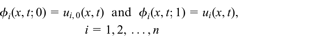
In view of equation $(21)$ , it is clear that when $q=0$ and $q=1$ , one has

$${\varphi }_i(x,t;0)=u_{i,0}(x,t)\mathrm{and}{\varphi }_i(x,t;1)=u_i(x,t),i=1,2,\dots ,n$$

Thus, as q deforms from 0 to 1, the functions ${\varphi }_i(x,t;q)$ vary from the initial approximations $u_{i,0}(x,t)$ to the exact solutions $u_i(x,t)$ .

Using Taylor series, one may have

$${\varphi }_i(x,t;q)=u_{i,0}(x,t)+\sum _{m=1}^{\infty }{u}_{i,m}(x,t)q^m$$

(22)

where

$$u_{i,m}(x,t)={\frac{1}{m!}\frac{{\partial }^m{\varphi }_i(x,t;q)}{\partial q^m}|}_{q=0}$$

As proved by Liao, ¹⁴ the convergence of the power series $(22)$ at $q=1$ depends on the choice of the auxiliary parameters, the auxiliary operators, the initial guesses, and the auxiliary functions. If these objects are chosen properly, then for $q=1$ , equation $(22)$ implies

$$u_i(x,t)=u_{i,0}(x,t)+\sum _{m=1}^{\infty }{u}_{i,m}(x,t)$$

(23)

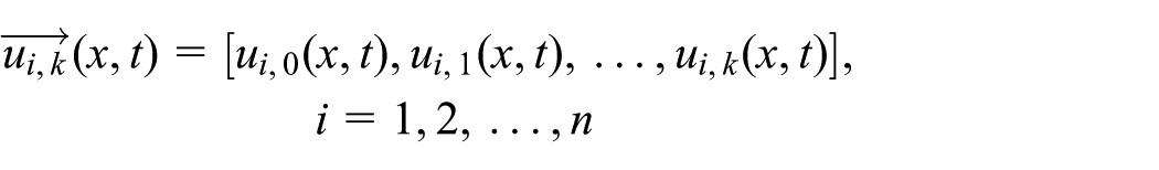
Define the vectors

$$\overrightarrow{u_{i,k}}(x,t)=[u_{i,0}(x,t),u_{i,1}(x,t),\dots ,u_{i,k}(x,t)],i=1,2,\dots ,n$$

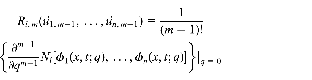
Then, the mth-order deformation equations are defined as follows (see Bataineh et al. ¹⁷ )

$$L_i[u_{i,m}(x,t)-{\chi }_m{u}_{i,m-1}(x,t)]={\hslash }_i{R}_{i,m}({\overrightarrow{u}}_{1,m-1},\dots ,{\overrightarrow{u}}_{n,m-1})$$

(24)

where

$${\chi }_m=\{\begin{array}{cc}0,\hfill & m\le 1\hfill \\ \multicolumn{1}{c}{1,}& m>1\hfill \end{array}$$

and

$$R_{i,m}({\overrightarrow{u}}_{1,m-1},\dots ,{\overrightarrow{u}}_{n,m-1})={\frac{1}{(m-1)!}\left\{\frac{{\partial }^{m-1}}{\partial q^{m-1}}{N}_i[{\varphi }_1(x,t;q),\dots ,{\varphi }_n(x,t;q)]\right\}|}_{q=0}$$

Now, the components $u_{i,m}(x,t)$ for $m\ge 1$ can be computed recursively by inverting the linear operators $L_i$ in equation $(24)$ along with the conditions from the original problem. For more details, see literature.^13–17

To apply the HAM to the systems $(1)-(3)$ , we choose appropriate initial approximations $u_0(x,t)\mathrm{and}{v}_0(x,t)$ satisfying the conditions $(2)\mathrm{and}(3)$ , and the linear operators

$$L_1[\varphi ]=L_2[\varphi ]=L[\varphi ]=\frac{1}{x}\frac{\partial }{\partial x}(x\frac{\partial }{\partial x}\varphi )$$

which satisfy

$$L[c_2-c_1\ln (x)]=0$$

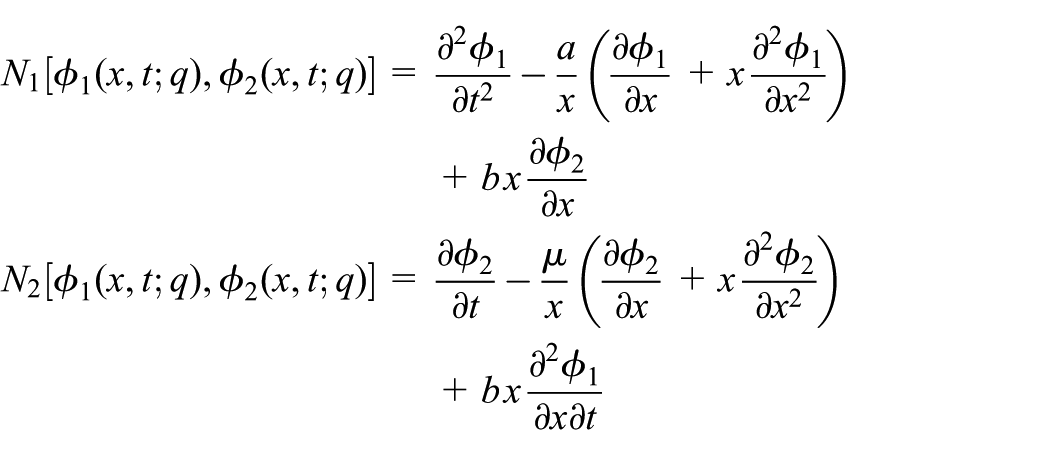
where $c_i$ , $i=1,2$ , are constants of integration. We also define the two operators $N_1$ and $N_2$ by

$$\begin{array}{l}{N}_1[{\varphi }_1(x,t;q),{\varphi }_2(x,t;q)]=\frac{{\partial }^2{\varphi }_1}{\partial t^2}-\frac{a}{x}(\frac{\partial {\varphi }_1}{\partial x}+x\frac{{\partial }^2{\varphi }_1}{\partial x^2})+bx\frac{\partial {\varphi }_2}{\partial x}\\ N_2[{\varphi }_1(x,t;q),{\varphi }_2(x,t;q)]=\frac{\partial {\varphi }_2}{\partial t}-\frac{\mu }{x}(\frac{\partial {\varphi }_2}{\partial x}+x\frac{{\partial }^2{\varphi }_2}{\partial x^2})+bx\frac{{\partial }^2{\varphi }_1}{\partial x\partial t}\end{array}$$

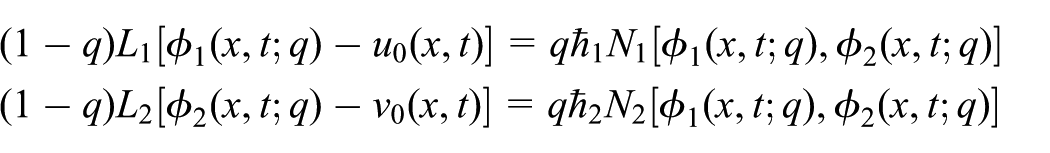
Now, the zeroth-order deformation equations can be constructed as

$$\begin{array}{l}(1-q)L_1[{\varphi }_1(x,t;q)-u_0(x,t)]=q{\hslash }_1{N}_1[{\varphi }_1(x,t;q),{\varphi }_2(x,t;q)]\\ (1-q)L_2[{\varphi }_2(x,t;q)-v_0(x,t)]=q{\hslash }_2{N}_2[{\varphi }_1(x,t;q),{\varphi }_2(x,t;q)]\end{array}$$

and in view of equation (24), the mth-order deformation equations are

$$L_1[u_m(x,t)-{\chi }_m{u}_{m-1}(x,t)]={\hslash }_1{R}_{1,m}({\overrightarrow{u}}_{m-1},{\overrightarrow{v}}_{m-1})$$

(25)

$$L_2[v_m(x,t)-{\chi }_m{v}_{m-1}(x,t)]={\hslash }_2{R}_{2,m}({\overrightarrow{u}}_{m-1},{\overrightarrow{v}}_{m-1})$$

(26)

where

$$\begin{array}{l}{R}_{1,m}({\overrightarrow{u}}_{m-1},{\overrightarrow{v}}_{m-1})={(u_{m-1})}_{tt}-\frac{a}{x}{(x{(u_{m-1})}_x)}_x+bx{(v_{m-1})}_x-(1-{\chi }_m)f(x,t)\\ R_{2,m}({\overrightarrow{u}}_{m-1},{\overrightarrow{v}}_{m-1})={(v_{m-1})}_t-\frac{\mu }{x}{(x{(v_{m-1})}_x)}_x+bx{(u_{m-1})}_{tx}-(1-{\chi }_m)g(x,t)\end{array}$$

and ${\hslash }_1$ and ${\hslash }_2$ are auxiliary parameters.

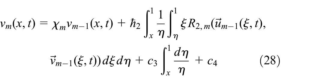
Now, applying the inverse of the operator L, namely, $L^{-1}(·)={\int }_x^1\frac{1}{\eta }{\int }_{\eta }^1\xi (·)d\xi d\eta$ , to both sides of equations (25) and (26), the solutions of the mth-order deformation equations $(25)$ and $(26)$ , for $m\ge 1$ , can be obtained recessively by employing the iterative schemes

$$u_m(x,t)={\chi }_m{u}_{m-1}(x,t)+{\hslash }_1{\int }_x^1\frac{1}{\eta }{\int }_{\eta }^1\xi R_{1,m}({\overrightarrow{u}}_{m-1}(\xi ,t),{\overrightarrow{v}}_{m-1}(\xi ,t))d\xi d\eta +c_1{\int }_x^1\frac{d\eta }{\eta }+c_2$$

(27)

$$v_m(x,t)={\chi }_m{v}_{m-1}(x,t)+{\hslash }_2{\int }_x^1\frac{1}{\eta }{\int }_{\eta }^1\xi R_{2,m}({\overrightarrow{u}}_{m-1}(\xi ,t),{\overrightarrow{v}}_{m-1}(\xi ,t))d\xi d\eta +c_3{\int }_x^1\frac{d\eta }{\eta }+c_4$$

(28)

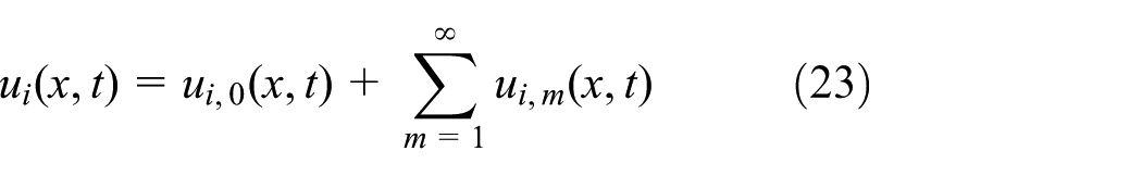
where $c_i,i=1,2,\dots ,4$ are constants of integration which can be determined using the conditions $(2)\mathrm{and}(3)$ , which lead to $c_i=0$ for $i=1,2,\dots ,4.$ Hence, the series solutions of the systems (1)–(3) are given by

$$u(x,t)=u_0(x,t)+\sum _{i=1}^{\infty }{u}_i(x,t)$$

and

$$v(x,t)=v_0(x,t)+\sum _{i=1}^{\infty }{v}_i(x,t)$$

Numerical examples

To test the efficiency of the method, we apply the iterative schemes (27) and (28) to two examples. In the first one, we consider a homogeneous system, and in the second one, we deal with a nonhomogeneous system. In both cases, we consider the same parameter values, namely, $a=b=\mu =1$ , and the auxiliary parameters as ${\hslash }_1={\hslash }_2=h$ .

Example 1: homogeneous system

Consider the systems $(1)-(3)$ with $f(x,t)=g(x,t)=0$ , initial conditions $u(x,0)=1-x,u_t(x,0)=1-x,v(x,0)=-4\ln (x),$ and boundary conditions as in (3). We choose the initial guesses as

$$u_0(x,t)=(1+t)(1-x),\mathrm{and}{v}_0(x,t)=-4\ln (x)$$

Then, in view of equations $(27)\mathrm{and}(28)$ , the first few terms of the series solutions are given by

$$\begin{array}{c}\multicolumn{1}{c}{u_1(x,t)=\frac{1}{9}h(-1+2t)(-1+x^3-3\ln (x))}\\ \multicolumn{1}{c}{u_2(x,t)=\frac{1}{9}h(-1+2t)(-1+x^3-3\ln (x))}\\ \multicolumn{1}{c}{-\frac{h^2}{7200}((-1+x)(433+433x}\\ \multicolumn{1}{c}{-767x^2+833x^3-292x^4-100x^5}\\ \multicolumn{1}{c}{+400t(-1-x+8x^2))-60(-6+40t+15x^4)\ln (x))}\end{array}$$

and

$$\begin{array}{l}{v}_1(x,t)=(h(\frac{1}{72}(-1+x)(7-144t-65x+25x^2+9x^3)\\ +(-\frac{2}{3}+2t+x^2)\ln (x)))\\ v_2(x,t)=\frac{1}{1800}(h((-1+x)(-25(-7+144t+65x\\ -25x^2-9x^3)+h(-827+3600t+973x\\ -977x^2-177x^3+48x^4))-60(-10(-2+6t+3x^2)\\ +h(-31+60t+15x^2))\ln (x))))\end{array}$$

Hence, the truncated series solutions of orders 1 and 2 are as follows

$$\begin{array}{c}\multicolumn{1}{c}{u^1(x,t)=\frac{1}{9}h(-1+2t)(-1+x^3-3\ln (x))+(1+t)\ln (x)}\\ \multicolumn{1}{c}{u^2(x,t)=\frac{2}{9}h(-1+2t)(-1+x^3-3\ln (x))+(1+t)}\\ \multicolumn{1}{c}{\ln (x)-\frac{1}{7200}(h^2((-1+x)(433+433x}\\ \multicolumn{1}{c}{-767x^2+833x^3-292x^4-100x^5+400t(-1-x+8x^2))}\\ \multicolumn{1}{c}{-60(-6+40t+15x^4)\ln (x))v^1(x,t)=(1-2t)(1-x)}\\ \multicolumn{1}{c}{+h(\frac{1}{72}(-1+x)(7-144t-65x+25x^2+9x^3)}\\ \multicolumn{1}{c}{+(\frac{-2}{3}+2t+x^2)\ln (x))}\\ \multicolumn{1}{c}{v^2(x,t)=(1-2t)(1-x)}\\ \multicolumn{1}{c}{+h(\frac{1}{72}(-1+x)(7-144t-65x+25x^2+9x^3)}\\ \multicolumn{1}{c}{+(\frac{-2}{3}+2t+x^2)\ln (x))}\\ \multicolumn{1}{c}{+\frac{1}{1800}(h((-1+x)(-25(-7+144t+65x}\\ \multicolumn{1}{c}{-25x^2-9x^3))+h(-827+3600t+973x}\\ \multicolumn{1}{c}{-977x^2-177x^3+48x^4))-60(-10(-2+6t+3x^2)}\\ \multicolumn{1}{c}{+h(-31+60t+15x^2))\ln (x)))}\end{array}$$

Figure 1 shows the h-curves based on the approximate solutions of order 9. It shows that the acceptable values of the auxiliary parameter h required for the convergence of the series solutions are $0.5\le h\le 1.4.$

Figure 1.

The h-curves for $u_{\mathrm{xxx}}(1,0)(--)$ and $v_{\mathrm{xxx}}(1,0)(-)$ based on ninth-order approximation.

Tables 1–8 show the values of the mth-order truncated series solutions $u^m(x,t)$ and $v^m(x,t)$ , computed for different values of the dependent variables x and t when $h=1$ . In fact, direct evaluation shows that the values of these solutions of any order $m\ge 1$ vanish at $x=1$ for all $t>0$ . These tables show that the method converges rapidly just after few terms.

Table 1.

Values of the truncated series solutions of order m at $t=0.1$ and $x=0.1,0.2,0.3$ .

m	x	$u^m(x,t)$	$v^m(x,t)$	x	$u^m(x,t)$	$v^m(x,t)$	x	$u^m(x,t)$	$v^m(x,t)$
1	0.1	−3.05807	1.94203	0.2	−2.11139	1.54145	0.3	−1.55894	1.25079
2		−3.49136	1.44657		−2.37479	1.27292		−1.72697	1.09644
3		−3.42633	1.37811		−2.34062	1.23671		−1.7084	1.07668
4		−3.41881	1.37811		−2.33686	1.23671		−1.7065	1.07668
5		−3.41881	1.37811		−2.33686	1.23671		−1.7065	1.07668
6		−3.41881	1.37811		−2.33686	1.23671		−1.7065	1.07668

Table 2.

Values of the truncated series solutions of order m at $t=0.1\mathrm{and}x=0.5,0.7,0.9$ .

m	x	$u(x,t{)}^m$	$v(x,t{)}^m$	x	$u^m(x,t)$	$v^m(x,t)$	x	$u^m(x,t)$	$v^m(x,t)$
1	0.5	−0.869523	0.77605	0.7	−0.429056	0.38819	0.9	−0.119904	0.0981165
2		−0.931524	0.728864		−0.443534	0.378839		−0.120501	0.0977819
3		−0.926897	0.723946		−0.442921	0.378196		−0.120493	0.0977737
4		−0.926517	0.723946		−0.442888	0.378196		−0.120493	0.0977737
5		−0.926517	0.723946		−0.442888	0.378196		−0.120493	0.0977737
6		−0.926517	0.723946		−0.442888	0.378196		−0.120493	0.0977737

Table 3.

Values of the truncated series solutions of order m at $t=1$ and $x=0.1,0.2,0.3$ .

m	x	$u^m(x,t)$	$v^m(x,t)$	x	$u^m(x,t)$	$v^m(x,t)$	x	$u^m(x,t)$	$v^m(x,t)$
1	0.1	−3.94864	−2.20263	0.2	−2.79262	−1.35554	0.3	−2.11473	−0.916364
2		−3.93686	−2.69809		−2.80679	−1.62407		−2.13647	−1.07071
3		−3.87183	−2.76654		−2.77262	−1.66028		−2.1179	−1.09047
4		−3.86431	−2.76654		−2.76886	−1.66028		−2.116	−1.09047
5		−3.86431	−2.76654		−2.76886	−1.66028		−2.116	−1.09047
6		−3.86431	−2.76654		−2.76886	−1.66028		−2.116	−1.09047

Table 4.

Values of the truncated series solutions of order m at $t=1\mathrm{and}x=0.5,0.7,0.9$ .

m	x	$u^m(x,t)$	$v^m(x,t)$	x	$u^m(x,t)$	$v^m(x,t)$	x	$u^m(x,t)$	$v^m(x,t)$
1	0.5	−1.25247	−0.471615	0.7	−0.667458	−0.253825	0.9	−0.205712	−0.0915324
2		−1.26902	−0.518801		−0.673034	−0.263176		−0.206001	−0.091867
3		−1.2644	−0.523719		−0.672421	−0.263818		−0.205993	−0.0918752
4		−1.26402	−0.523719		−0.672388	−0.263818		−0.205993	−0.0918752
5		−1.26402	−0.523719		−0.672388	−0.263818		−0.205993	−0.0918752
6		−1.26402	−0.523719		−0.672388	−0.263818		−0.205993	−0.0918752

Table 5.

Values of the truncated series solutions of order m at $t=5$ and $x=0.1,0.2,0.3$ .

m	x	$u^m(x,t)$	$v^m(x,t)$	x	$u^m(x,t)$	$v^m(x,t)$	x	$u^m(x,t)$	$v^m(x,t)$
1	0.1	−7.90676	−20.6233	0.2	−5.82031	−14.231	0.3	−4.58492	−10.5481
2		−5.91686	−21.1188		−4.72679	−14.4996		−3.95647	−10.7025
3		−5.85183	−21.1872		−4.69262	−14.5358		−3.9379	−10.7223
4		−5.84431	−21.1872		−4.68886	−14.5358		−3.936	−10.7223
5		−5.84431	−21.1872		−4.68886	−14.5358		−3.936	−10.7223
6		−5.84431	−21.1872		−4.68886	−14.5358		−3.936	−10.7223

Table 6.

Values of the truncated series solutions of order m at $t=5$ and $x=0.5,0.7,0.9$ .

m	x	$u^m(x,t)$	$v^m(x,t)$	x	$u^m(x,t)$	$v^m(x,t)$	x	$u^m(x,t)$	$v^m(x,t)$
1	0.5	−2.95444	−6.01679	0.7	−1.72702	−3.10722	0.9	−0.587082	−0.934417
2		−2.76902	−6.06398		−1.69303	−3.11658		−0.586001	−0.934751
3		−2.7644	−6.0689		−1.69242	−3.11722		−0.585993	−0.934759
4		−2.76402	−6.0689		−1.69239	−3.11722		−0.585993	−0.934759
5		−2.76402	−6.0689		−1.69239	−3.11722		−0.585993	−0.934759
6		−2.76402	−6.0689		−1.69239	−3.11722		−0.585993	−0.934759

Table 7.

Values of the truncated series solutions of order m at $t=10$ and $x=0.1,0.2,0.3$ .

m	x	$u^m(x,t)$	$v^m(x,t)$	x	$u^m(x,t)$	$v^m(x,t)$	x	$u^m(x,t)$	$v^m(x,t)$
1	0.1	−12.8544	−43.6492	0.2	−9.60493	−30.3254	0.3	−7.67265	−22.5879
2		−8.39186	−44.1446		−7.12679	−30.594		−6.23147	−22.7422
3		−8.32683	−44.2131		−7.09262	−30.6302		−6.2129	−22.762
4		−8.31931	−44.2131		−7.08886	−30.6302		−6.211	−22.762
5		−8.31931	−44.2131		−7.08886	−30.6302		−6.211	−22.762
6		−8.31931	−44.2131		−7.08886	−30.6302		−6.211	−22.762

Table 8.

Values of the truncated series solutions of order m at $t=10$ and $x=0.5,0.7,0.9$ .

m	x	$u^m(x,t)$	$v^m(x,t)$	x	$u^m(x,t)$	$v^m(x,t)$	x	$u^m(x,t)$	$v^m(x,t)$
1	0.5	−5.08191	−12.9483	0.7	−3.05148	−6.67397	0.9	−1.06379	−1.98802
2		−4.64402	−12.9955		−2.96803	−6.68332		−1.061	−1.98836
3		−4.6394	−13.0004		−2.96742	−6.68397		−1.06099	−1.98836
4		−4.63902	−13.0004		−2.96739	−6.68397		−1.06099	−1.98836
5		−4.63902	−13.0004		−2.96739	−6.68397		−1.06099	−1.98836
6		−4.63902	−13.0004		−2.96739	−6.68397		−1.06099	−1.98836

Example 2: nonhomogeneous system

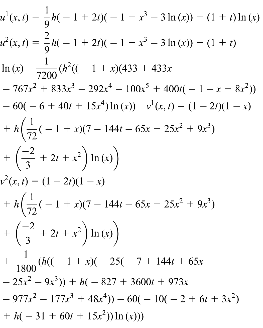
Consider the systems $(1)-(3)$ with $f(x,t)=0,g(x,t)=-2x^2-4\mathrm{lnx},$ initial conditions $u(x,0)=1-x^2,u_t(x,0)=1-x^2,v(x,0)=(1-x)$ , and boundary conditions as in (3). Let us take the initial guesses as

$$u_0(x,t)=(1+t)(1-x^2),\mathrm{and}{v}_0(x,t)=(1+t^2)(1-x)$$

Then, in view of equations (22) and (23), the first few terms of the series solutions are given by

$$\begin{array}{l}{u}_1(x,t)=\frac{1}{9}h(-8-9t+t^2+9(1+t)x^2-(1+t^2)x^3+3(-5+(-6+t)t)\ln (x))\\ u_2(x,t)=\frac{1}{3600}(h(400(-8-9t+t^2+9(1+t)x^2-(1+t^2)x^3+3(-5+(-6+t)t)\\ \ln (x))+h(3682+3771t+100t^2\\ -100(5+3t)(8+3t)x^2+800(1+t^2)x^3+225(-2+t)x^4\\ -32(1+3t)x^5+30(217+246t-20t^2+20x^2+15x^4)\ln (x))))\end{array}$$

and

$$\begin{array}{c}{v}_1(x,t)=\frac{1}{18}h((-1+x)(18t^2-18x+t(5+5x-4x^2))\hfill \\ \multicolumn{1}{c}{-6(t+3t^2-3x^2)\ln (x))}\\ v_2(x,t)=\frac{1}{7200}(h(400((-1+x)(18t^2-18x\hfill \\ \multicolumn{1}{c}{+t(5+5x-4x^2))-6(t+3t^2-3x^2)\ln (x))}\\ +h(2439-7200t^2(-1+x)+x(-7200+3700x\hfill \\ \multicolumn{1}{c}{+1125x^3-64x^4)-32t(19}\\ +x^2(75-100x+6x^3))+60(57-4t+120t^2\hfill \\ \multicolumn{1}{c}{-10(13+6t)x^2)\ln (x))))}\end{array}$$

Hence, the truncated series solutions of orders 1 and 2 are as follows

$$\begin{array}{l}{u}^1(x,t)=(1+t)(1-x^2)+\frac{1}{9}h(-8-9t+t^2+9(1+t)\\ x^2-(1+t^2)x^3+3(-5+(-6+t)t)\ln (x))\\ u^2(x,t)=(1+t)(1-x^2)+\frac{1}{9}h(-8-9t+t^2+9(1+t)\\ x^2-(1+t^2)x^3+3(-5+(-6+t)t)\ln (x)\\ +\frac{1}{3600}(h(400(-8-9t+t^2+9(1+t)x^2-(1+t^2)x^3\\ +3(-5+(-6+t)t)\ln (x))+h(3682+3771t+100t^2\\ -100(5+3t)(8+3t)x^2+800(1+t^2)x^3+225(-2+t)x^4\\ -32(1+3t)x^5+30(217+246t-20t^2+20x^2+15x^4)\ln (x)))))\end{array}$$

and

$$\begin{array}{l}{v}^1(x,t)=(1+t^2)(1-x)+\frac{1}{18}h((-1+x)(18t^2-18x\\ +t(5+5x-4x^2))-6(t+3t^2-3x^2)ln(x))\\ v^2(x,t)=(1+t^2)(1-x)+\frac{1}{18}h((-1+x)(18t^2-18x\\ +t(5+5x-4x^2))-6(t+3t^2-3x^2)\ln (x))\\ +\frac{1}{7200}(h(400((-1+x)(18t^2-18x+t(5+5x-4x^2))\\ -6(t+3t^2-3x^2)\ln (x))+h(2439-7200t^2(-1+x)\\ +x(-7200+3700x+1125x^3-64x^4)-32t(19+x^2(75\\ -100x+6x^3))+60(57-4t+120t^2-10(13+6t)x^2)\ln (x))))\end{array}$$

Figure 2 shows the h-curve based on the approximate solutions of order 9. It shows that the acceptable values of the auxiliary parameter h required for the convergence of the series solutions are $0.4\le h\le 1.5$ .

Figure 2.

The h-curves for $u_{\mathrm{xxx}}(1,0)(--)$ and $v_{\mathrm{xxx}}(1,0)(-)$ based on ninth-order approximation.

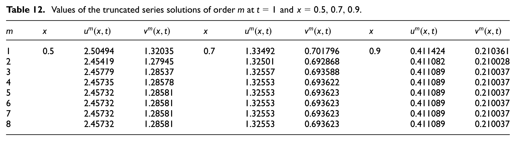
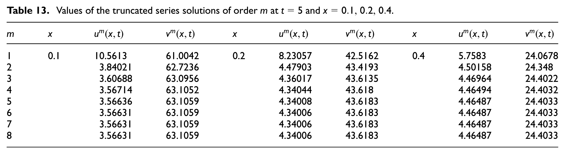
Tables 9–16 show the values of the mth order truncated series solutions $u^m(x,t)$ and $v^m(x,t)$ , computed for different values of the dependent variables x and t when $h=1$ . In fact, direct evaluation shows that the values of these solutions of any order $m\ge 1$ vanish at $x=1$ for all $t>0$ . These tables show that the method converges rapidly just after few terms.

Table 9.

Values of the truncated series solutions of order m at $t=0.1$ and $x=0.1,0.2,0.4$ .

m	x	$u^m(x,t)$	$v^m(x,t)$	x	$u^m(x,t)$	$v^m(x,t)$	x	$u^m(x,t)$	$v^m(x,t)$
1	0.1	4.40259	1.03945	0.2	3.11024	0.939409	0.4	1.8124	0.711899
2		4.19609	0.331094		2.99631	0.526697		1.77365	0.562527
3		4.28141	0.367606		3.04491	0.543447		1.78919	0.566162
4		4.27853	0.377201		3.04358	0.547972		1.78893	0.567161
5		4.27775	0.377881		3.04322	0.548293		1.78886	0.567227
6		4.27769	0.377881		3.0432	0.548293		1.78885	0.567227
7		4.27769	0.377881		3.0432	0.548293		1.78885	0.567227
8		4.27769	0.377881		3.0432	0.548293		1.78885	0.567227

Table 10.

Values of the truncated series solutions of order m at $t=0.1\mathrm{and}x=0.5,0.7,0.9$ .

m	x	$u^m(x,t)$	$v^m(x,t)$	x	$u^m(x,t)$	$v^m(x,t)$	x	$u^m(x,t)$	$v^m(x,t)$
1	0.5	1.38976	0.588694	0.7	0.738334	0.339785	0.9	0.226734	0.105746
2		1.36843	0.505318		0.733908	0.322441		0.226568	0.105112
3		1.3762	0.50682		0.73501	0.322583		0.226583	0.105113
4		1.3761	0.507227		0.735004	0.322617		0.226583	0.105113
5		1.37607	0.507252		0.735002	0.322618		0.226583	0.105113
6		1.37607	0.507252		0.735002	0.322618		0.226583	0.105113
7		1.37607	0.507252		0.735002	0.322618		0.226583	0.105113
8		1.37607	0.507252		0.735002	0.322618		0.226583	0.105113

Table 11.

Values of the truncated series solutions of order m at $t=1$ and $x=0.1,0.2,0.4$ .

m	x	$u^m(x,t)$	$v^m(x,t)$	x	$u^m(x,t)$	$v^m(x,t)$	x	$u^m(x,t)$	$v^m(x,t)$
1	0.1	7.89728	3.76409	0.2	5.58524	2.78198	0.4	3.2623	1.70311
2		7.38437	3.50164		5.30164	2.61095		3.16802	1.63264
3		7.41117	3.59977		5.31948	2.66029		3.17484	1.64557
4		7.40152	3.60936		5.31477	2.66482		3.17376	1.64657
5		7.40074	3.61004		5.31441	2.66514		3.17369	1.64663
6		7.40068	3.61004		5.31439	2.66514		3.17369	1.64663
7		7.40068	3.61004		5.31439	2.66514		3.17369	1.64663
8		7.40068	3.61004		5.31439	2.66514		3.17369	1.64663

Table 12.

Values of the truncated series solutions of order m at $t=1\mathrm{and}x=0.5,0.7,0.9$ .

m	x	$u^m(x,t)$	$v^m(x,t)$	x	$u^m(x,t)$	$v^m(x,t)$	x	$u^m(x,t)$	$v^m(x,t)$
1	0.5	2.50494	1.32035	0.7	1.33492	0.701796	0.9	0.411424	0.210361
2		2.45419	1.27945		1.32501	0.692868		0.411082	0.210028
3		2.45779	1.28537		1.32557	0.693588		0.411089	0.210037
4		2.45735	1.28578		1.32553	0.693622		0.411089	0.210037
5		2.45732	1.28581		1.32553	0.693623		0.411089	0.210037
6		2.45732	1.28581		1.32553	0.693623		0.411089	0.210037
7		2.45732	1.28581		1.32553	0.693623		0.411089	0.210037
8		2.45732	1.28581		1.32553	0.693623		0.411089	0.210037

Table 13.

Values of the truncated series solutions of order m at $t=5$ and $x=0.1,0.2,0.4$ .

m	x	$u^m(x,t)$	$v^m(x,t)$	x	$u^m(x,t)$	$v^m(x,t)$	x	$u^m(x,t)$	$v^m(x,t)$
1	0.1	10.5613	61.0042	0.2	8.23057	42.5162	0.4	5.7583	24.0678
2		3.84021	62.7236		4.47903	43.4193		4.50158	24.348
3		3.60688	63.0956		4.36017	43.6135		4.46964	24.4022
4		3.56714	63.1052		4.34044	43.618		4.46494	24.4032
5		3.56636	63.1059		4.34008	43.6183		4.46487	24.4033
6		3.56631	63.1059		4.34006	43.6183		4.46487	24.4033
7		3.56631	63.1059		4.34006	43.6183		4.46487	24.4033
8		3.56631	63.1059		4.34006	43.6183		4.46487	24.4033

Table 14.

Values of the truncated series solutions of order m at $t=5\mathrm{and}x=0.5,0.7,0.9$ .

m	x	$u^m(x,t)$	$v^m(x,t)$	x	$u^m(x,t)$	$v^m(x,t)$	x	$u^m(x,t)$	$v^m(x,t)$
1	0.5	4.83827	18.1579	0.7	3.08692	9.30156	0.9	1.13409	2.74038
2		4.16193	18.3057		2.95574	9.33004		1.12961	2.74139
3		4.14702	18.3313		2.95384	9.33333		1.12958	2.74143
4		4.14506	18.3317		2.95367	9.33336		1.12958	2.74143
5		4.14504	18.3317		2.95367	9.33336		1.12958	2.74143
6		4.14503	18.3317		2.95367	9.33336		1.12958	2.74143
7		4.14503	18.3317		2.95367	9.33336		1.12958	2.74143
8		4.14503	18.3317		2.95367	9.33336		1.12958	2.74143

Table 15.

Values of the truncated series solutions of order m at $t=10$ and $x=0.1,0.2,0.4$ .

m	x	$u^m(x,t)$	$v^m(x,t)$	x	$u^m(x,t)$	$v^m(x,t)$	x	$u^m(x,t)$	$v^m(x,t)$
1	0.1	−15.6525	236.171	0.2	−7.64433	164.609	0.4	−0.186059	93.2568
2		−41.2607	240.367		−21.9616	166.854		−4.99802	93.9753
3		−41.8191	241.082		−22.2513	167.23		−5.07841	94.0811
4		−41.8965	241.091		−22.2898	167.234		−5.08763	94.0821
5		−41.8973	241.092		−22.2902	167.234		−5.0877	94.0822
6		−41.8973	241.092		−22.2902	167.234		−5.0877	94.0822
7		−41.8973	241.092		−22.2902	167.234		−5.0877	94.0822
8		−41.8973	241.092		−22.2902	167.234		−5.0877	94.0822

Table 16.

Values of the truncated series solutions of order m at $t=10\mathrm{and}x=0.5,0.7,0.9$ .

m	x	$u^m(x,t)$	$v^m(x,t)$	x	$u^m(x,t)$	$v^m(x,t)$	x	$u^m(x,t)$	$v^m(x,t)$
1	0.5	1.73273	70.3964	0.7	3.21179	36.1016	0.9	1.81202	10.6441
2		−0.861708	70.7801		2.70647	36.1769		1.79465	10.6468
3		−0.899747	70.8303		2.7015	36.1834		1.79459	10.6469
4		−0.903611	70.8307		2.70116	36.1834		1.79459	10.6469
5		−0.903637	70.8308		2.70116	36.1834		1.79459	10.6469
6		−0.903638	70.8308		2.70116	36.1834		1.79459	10.6469
7		−0.903638	70.8308		2.70116	36.1834		1.79459	10.6469
8		−0.903638	70.8308		2.70116	36.1834		1.79459	10.6469

Conclusion

Some well-posed results of a linear singular thermoelastic system are obtained. Moreover, the system is solved numerically by HAM. The derived schemes are tested numerically using two examples, one of them is homogeneous and the second one is nonhomogeneous. These examples show that the truncated series solutions converge rapidly just after few terms, showing the efficiency and effectiveness of the HAM method.