Sage Journals: Discover world-class research

Abstract

In this article, we present an efficient method for solving nonlinear Fredholm integral equations of the second kind. The proposed method is based on the Galerkin method and transformations of shifted Chebyshev polynomials. This method is simple and computationally very attractive. Finally, illustrative examples and also the application of the proposed method to solve a functional differential equation are presented to show the validity and applicability of the technique.

Keywords

Hammerstein equations nonlinear Fredholm integral equation shifted Chebyshev polynomials Taylor expansion Galerkin method

Introduction

Integral equations play a very vital role in science, such as numerous problems in mathematics and engineering (see, for example,^1–5 and the references therein). For instance, one of the most important domains of applications of the ideas and methods of nonlinear functional analysis and also the theory of nonlinear operators of monotone type is integral equations of the Fredholm–Hammerstein.⁶ Furthermore, this kind of integral equations appears in nonlinear physical phenomena such as electro-magnetic fluid dynamics, reformulation of boundary value problems (BVPs) with a nonlinear boundary condition.⁷ This equation is as follows

u (t) - \int_{a}^{b} K (t, y) {[u (y)]}^{m} dy = f (t)

(1)

where $f (t) \in L^{2} [a, b] and K (t, y) \in L^{2} [a, b] \times [a, b]$ are known functions, $u (t)$ is the unknown function to be determined, $t \in I = [a, b]$ , and $m > 1$ is a positive integer.⁸ Since we use the shifted Chebyshev polynomials and these polynomials are an orthogonal set on the interval $[0, 1]$ , throughout this article, without loss of generality, we assume that $a = 0 and b = 1$ .

Numerous numerical methods have been proposed for approximating the solution of above Fredholm–Hammerstein integral equations. For example, Tricomi⁹ (section 4.6) introduced the classical method of successive approximations. Kumar and Sloan¹⁰ have considered the solution of the Fredholm–Hammerstein integral equations and presented a collocation-type method to solve it. Brunner¹¹ used this method for the numerical solution of nonlinear Volterra integral and integro-differential equations. Guoqiang¹² obtained the asymptotic error expansion of this method and showed that the Richardson’s extrapolation can be performed on the solution and this will greatly increase the accuracy of numerical solution. Elnagar and Kazemi¹³ investigated the Chebyshev spectral method to an equivalent equation of nonlinear Volterra–Hammerstein integral equations and discussed some convergence results. Hernandez et al.¹⁴ applied a one-parametric family of secant-type iterations for equation (1) and established a semilocal convergence result for these iterations by means of a technique based on a new system of recurrence relations. Kaneko et al.¹⁵ developed the Petrov–Galerkin method and the iterated Petrov–Galerkin method for equation (1) and established a framework for fast algorithms to obtaining approximate solutions based on Alpert’s Wavelets. Contea and Prete¹⁶ proposed discrete collocation methods for Volterra integral equations of Hammerstein type, where the Laplace transform of the kernel rather than the convolution kernel itself is known a priori. For details of the application of the spectral methods for solving some differential equations,^17–21 In recent years, numerous numerical methods have been proposed to find Hammerstein integral equations. These methods include Nyström type methods,^22,23 projection methods,^24,25 methods of special functions,^25–29 wavelets,^30–41 homotopy techniques, the Adomian decomposition method,^42,43 Toeplitz matrix method,⁴⁴ polynomial interpolation procedures,^45–47 and multigrid methods.⁴⁸ The main problem for solution of equation (1) is $[u (y)]^{m}$ . Some methods used quadrature formula methods and spline approximations (e.g. see the studies by Maleknejad and Lotfi⁴⁵). Some methods considered $[u (y)]^{m}$ as an independent variable (e.g. see equation (7) in Babolian and Shahsavaran³⁹). Some methods applied equivalent equation as follows

{[u (y)]}^{m} = ψ (y, u (y)) = ψ (y, \sum_{i = 1}^{n} c_{i} \int_{a}^{b} K (t, y) b_{i} (y) dy + f (y))

These require a huge number of arithmetic operators, high computational costs, and a large storage capacity.^13,15,34

Some methods also used operational vector. For example, in Mahmoudi,³³ equation (1) is investigated using Legendre wavelets basis. The method proposed there only works under the condition that the operational vector $Y^{*}$ is a vector function of Y; moreover, this function must be explicitly known (see equation (4.2) in Mahmoudi³³). Generally, it is difficult to meet this requirement in practice.

The existing results presented above for solving the Hammerstein integral equations motivate the study of this type of functional integral equations. Therefore, the main contribution of this article is to correct these models, with regard to the computational costs. In this article, we present an efficient algorithmic method which is new and different from all the existing methods. Our method is based on Galerkin methods and transformations of orthogonal polynomials. This method is very simple to apply and offers several advantages in reducing computational costs.

This article is organized as follows. In sections “Properties of shifted Chebyshev polynomials” and “Galerkin method,” we, respectively, give an overview of shifted Chebyshev polynomials and Galerkin method with their relevant properties needed hereafter. In section “Main results,” the way of constructing the proposed method for solving Hammerstein integral equations is described. Numerical experiments and also the application of the proposed method to solve a BVP are presented in section “Illustrative examples.” Finally, conclusions are given in section “Conclusion.”

Solving the Hammerstein integral equations

Properties of shifted Chebyshev polynomials

Chebyshev polynomials are important in approximation theory and numerical analysis and in some quadrature rules based on these polynomials such as Gauss–Chebyshev rule that appears in the theory of numerical integration.^49–51

Consider the well-known shifted Chebyshev polynomials of order $n, T_{n} (x),$ which is derived from the following recursive formula (for $x \in [0, 1]$ )

\begin{matrix} T_{0} (x) = 1 \\ T_{1} (x) = 2 x - 1 \\ T_{n} (x) = 2 (2 x - 1) T_{n - 1} - T_{n - 2} \end{matrix}

(2)

Moreover, these polynomials are orthogonal with respect to the weight function $ω (x) = \frac{1}{\sqrt{x (1 - x)}}$ on the interval [0, 1] and satisfy

\int_{0}^{1} \frac{T_{i} T_{j}}{\sqrt{x (1 - x)}} = ϒ_{i} δ_{ij}

where $δ_{ij}$ is the Kronecker delta and

ϒ_{i} = {\begin{matrix} π / 2, i \neq 0 \\ π, i = 0 \end{matrix}

Furthermore, for $x^{n}$ in terms of shifted Chebyshev polynomials, we have the following formula

x^{n} = 2^{1 - 2 n} {\frac{1}{2} (\begin{matrix} 2 n \\ n \end{matrix}) T_{0} (x) + \sum_{k = 0}^{n - 1} (\begin{matrix} 2 n \\ k \end{matrix}) T_{n - k} (x)}, n \geq 1

(3)

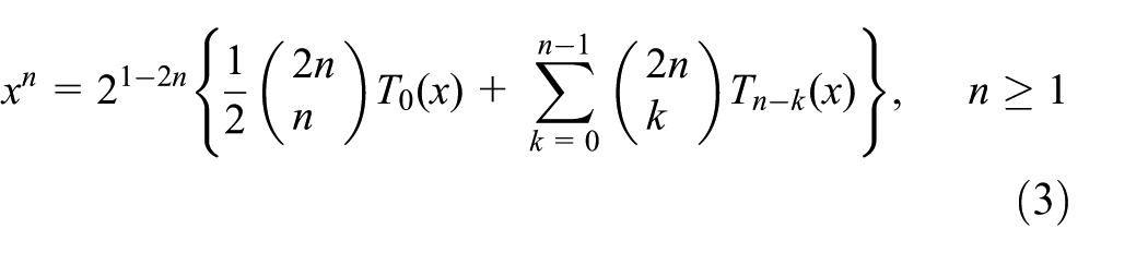
The first few powers in terms of shifted Chebyshev polynomials are (see the work by Mason and Handscomb (section 2.3)⁵⁰ and Synder⁵¹)

\begin{matrix} 1 = T_{0} (x) \\ x = \frac{1}{2} [T_{0} (x) + T_{1} (x)] \\ x^{2} = \frac{1}{8} [3 T_{0} (x) + 4 T_{1} (x) + T_{2} (x)] \\ x^{3} = \frac{1}{32} [10 T_{0} (x) + 15 T_{1} (x) + 6 T_{2} (x) + T_{3} (x)] \\ x^{4} = \frac{1}{128} [35 T_{0} (x) + 56 T_{1} (x) + 28 T_{2} (x) + 8 T_{3} (x) + T_{4} (x)] \\ ⋮ \end{matrix}

For some recent application of these polynomials, see Doha et al.⁵² and Bhrawy and Alofi.⁵³

Galerkin method

The basic idea of the weighted residual method is to assume that the unknown function $u (t)$ in equation (1) can be approximated by the sum of $N + 1$ trail functions $b_{i} (t)$ , that is

u (t) \approx u_{app} = \sum_{i = 0}^{N} c_{i} b_{i} (t)

(4)

And by assuming that the function $u_{app}$ is a linear combination of $b_{i} (t)$ , its expansion coefficients $c_{i}$ are to be determined uniquely.

Substituting the approximate solution given by equation (4) into equation (1), the result is the residual function defined by

E (t, c_{i}) = L [u_{app}] - f (t)

(5)

where

L [u_{app}] = u_{app} - \int_{a}^{b} K (t, y) {[u_{app}]}^{m} dy

(6)

Since the residual function is identically equal to zero for the exact solution, the challenge is to choose the coefficients $c_{i}$ so that the residual function is minimized. In integral form, this can be achieved with the following condition

\int_{a}^{b} ω_{i} (t) E (t, c_{i}) dt = 0

(7)

where $ω_{i} (t)$ is the weight function. The Galerkin approach makes the residual $E (t, c_{i})$ orthogonal to $N + 1$ , given the independent function on the domain $[a, b]$ . In this approach, the weighting function is chosen to be identical to the trail functions.

Main results

Consider the approximate solution given by equation (4) which is $b_{i} (t) = t^{i}$ , that is

u_{app} = \sum_{i = 0}^{N} c_{i} t^{i}

(8)

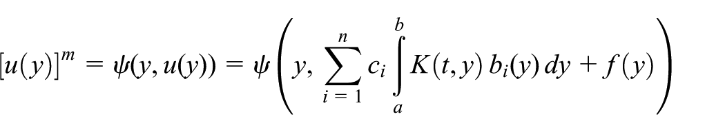
Then, by equation (1), we have

ψ (y, u (y)) = [u_{app}]^{m} = {[\sum_{i = 0}^{N} c_{i} y^{i}]}^{m}

(9)

Now, by Taylor expansion of $ψ (t, y)$ about zero, we can write

\begin{matrix} ψ (y, u (y)) = ψ (y = 0, u (y)) + (\frac{\partial}{\partial y} ψ (y = 0, u (y))) y + (\frac{1}{2!} \frac{\partial^{2}}{\partial y^{2}} ψ (y = 0, u (y))) y^{2} \\ \begin{matrix} + \dots + (\frac{1}{N!} \frac{\partial^{N}}{\partial y^{N}} ψ (y = 0, u (y))) y^{N} + \dots + (\frac{1}{(D)!} \frac{\partial^{D}}{\partial y^{D}} ψ (y = 0, u (y))) y^{D} \end{matrix} \end{matrix}

(10)

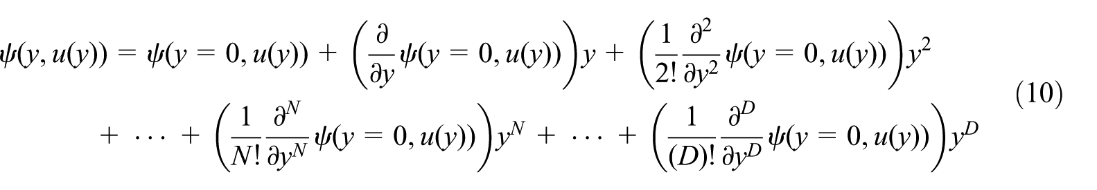
where $D = m \cdot N$ .

Then, we have

\begin{matrix} ψ (y, u (y)) = {({[\sum_{i = 0}^{N} c_{i} y^{i}]}^{m})}_{y = 0} + {(\frac{\partial}{\partial y} {[\sum_{i = 0}^{N} c_{i} y^{i}]}^{m})}_{y = 0} y + {(\frac{1}{2!} \frac{\partial^{2}}{\partial y^{2}} {[\sum_{i = 0}^{N} c_{i} y^{i}]}^{m})}_{y = 0} y^{2} \\ \begin{matrix} + \dots + {(\frac{1}{N!} \frac{\partial^{N}}{\partial y^{N}} {[\sum_{i = 0}^{N} c_{i} y^{i}]}^{m})}_{y = 0} y^{N} + \dots + {(\frac{1}{D!} \frac{\partial^{D}}{\partial y^{D}} {[\sum_{i = 0}^{N} c_{i} y^{i}]}^{m})}_{y = 0} y^{D} \end{matrix} \end{matrix}

(11)

Moreover, since

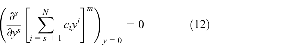
{(\frac{\partial^{s}}{\partial y^{s}} {[\sum_{i = s + 1}^{N} c_{i} y^{i}]}^{m})}_{y = 0} = 0

(12)

We obtain the following expansion for the above relation

\begin{matrix} ψ (y, u (y)) = ([c_{0}]^{m}) + {(\frac{\partial}{\partial y} {[c_{0} + c_{1} y]}^{m})}_{y = 0} y + {(\frac{1}{2!} \frac{\partial^{2}}{\partial y^{2}} {[\sum_{i = 0}^{2} c_{i} y^{i}]}^{m})}_{y = 0} y^{2} + {(\frac{1}{3!} \frac{\partial^{3}}{\partial y^{3}} {[\sum_{i = 0}^{3} c_{i} y^{i}]}^{m})}_{y = 0} y^{3} \\ + \dots + {(\frac{1}{N!} \frac{\partial^{N}}{\partial y^{N}} {[\sum_{i = 0}^{N} c_{i} y^{i}]}^{m})}_{y = 0} y^{N} + {(\frac{1}{(N + 1)!} \frac{\partial^{N + 1}}{\partial y^{N + 1}} {[\sum_{i = 0}^{N} c_{i} y^{i}]}^{m})}_{y = 0} y^{N + 1} + \dots + {(\frac{1}{D!} \frac{\partial^{D}}{\partial y^{D}} {[\sum_{i = 0}^{N} c_{i} y^{i}]}^{m})}_{y = 0} y^{D} \end{matrix}

Therefore, we can write

[u_{app}]^{m} = \sum_{i = 0}^{D} P_{i} y^{i}

(13)

where

P_{s} = {\begin{matrix} {(\frac{1}{s!} \frac{\partial^{s}}{\partial y^{s}} {[\sum_{i = 0}^{s} c_{i} y^{i}]}^{m})}_{y = 0}, & for s = 0, 1, \dots, N \\ {(\frac{1}{s!} \frac{\partial^{s}}{\partial y^{s}} {[\sum_{i = 0}^{N} c_{i} y^{i}]}^{m})}_{y = 0}, & for s = N + 1, \dots, D \end{matrix}

(14)

Now, by transformations of orthogonal polynomials based on formula (3), we will obtain an efficient method to solve equation (1). This method is as follows.

Algorithm 1

Step 1. Choose $u_{app} = \sum_{i = 0}^{N} c_{i} t^{i}$ and $[u_{app}]^{m} = \sum_{i = 0}^{D} P_{i} y^{i}$ .

Step 2. Use formula (3) and set $u_{app} = \sum_{i = 0}^{N} α_{i} T_{i} (t)$ and $[u_{app}]^{m} = \sum_{i = 0}^{D} β_{i} T_{i} (y)$

Step 3. Apply Galerkin method and solve the following nonlinear equations:

ϒ_{j} α_{j} - \sum_{i = 0}^{D} β_{i} K_{i, j} = f_{j}, \begin{matrix} j = 0, \dots, N, \begin{matrix} i = 0, \dots, D \end{matrix} \end{matrix}

(15)

where,

f_{j} = \int_{0}^{1} ω (t) f (t) P_{j} (t) dt

(16)

K_{i, j} = \int_{0}^{1} \int_{0}^{1} ω (t) K (t, y) P_{i} (y) P_{j} (t) dydt

(17)

Illustrative examples

In this section, we give some numerical experiments to illustrate the results obtained in previous sections.

Example 1

Consider the following nonlinear Fredholm–Hammerstein integral equation

u (t) = - \frac{1}{4} (t - 4 e^{t} + t e^{2}) + \int_{0}^{1} ty {[u (y)]}^{2} dy

with exact solution $u (t) = e^{t}$ .

To solve the above problem using our method, we do the following steps:

Let us consider $N = 2$ . Then, we construct trail space as follows

u_{app} = \sum_{i = 0}^{2} c_{i} t^{i} = c_{0} + c_{1} x + c_{2} x^{2}

and using formula (3), we have

u_{app} = \sum_{i = 0}^{2} α_{i} T_{i} (t)

where

α_{0} = c_{0} + \frac{1}{2} c_{1} + \frac{3}{8} c_{2}, α_{1} = \frac{1}{2} c_{1} + \frac{1}{2} c_{2}, α_{2} = \frac{1}{8} c_{2}

Similarly,

[u_{app}]^{2} = \sum_{i = 0}^{4} P_{i} y^{i}

where

P_{0} = c_{0}^{2}, P_{1} = 2 c_{0} c_{1}, P_{2} = c_{1}^{2} + 2 c_{0} c_{2}, P_{3} = 2 c_{1} c_{2}, P_{4} = c_{1}^{2}

and using formula (3), we have

[u_{app}]^{2} = \sum_{i = 0}^{4} β_{i} T_{i} (y)

where

\begin{matrix} β_{0} = P_{0} + \frac{1}{2} P_{1} + \frac{3}{8} P_{2} + \frac{10}{32} P_{3} + \frac{35}{128} P_{4} \\ β_{1} = \frac{1}{2} P_{1} + \frac{1}{2} P_{2} + \frac{15}{32} P_{3} + \frac{56}{128} P_{4} \\ β_{2} = \frac{1}{8} P_{2} + \frac{6}{32} P_{3} + \frac{28}{128} P_{4} \\ β_{3} = \frac{1}{32} P_{3} + \frac{8}{128} P_{4} \\ β_{4} = \frac{1}{128} P_{4} \end{matrix}

So, we have

\sum_{i = 0}^{2} α_{i} T_{i} (t) - \int_{0}^{1} ty [\sum_{i = 0}^{4} β_{i} T_{i} (y)] dy = - \frac{1}{4} (t - 4 e^{t} + t e^{2})

Now, we multiply both sides of the above relation with ${ω (t) T_{j} (t)}_{j = 0}^{2}$ ; from the orthogonality of shifted Chebyshev polynomials, we obtain the following nonlinear equations

\begin{array}{l} [\begin{matrix} π α_{0} \\ \frac{π}{2} α_{1} \\ \frac{π}{2} α_{2} \end{matrix}] - [\begin{matrix} π / 4 & π / 12 & - π / 12 & - π / 20 & - π / 60 \\ π / 8 & π / 24 & - π / 24 & - π / 40 & - π / 120 \\ 0 & 0 & 0 & 0 & 0 \end{matrix}] \\ [\begin{matrix} β_{0} \\ β_{1} \\ β_{2} \\ β_{3} \\ β_{4} \end{matrix}] = [\begin{matrix} 2741 / 1238 \\ - 828 / 2659 \\ 98 / 593 \\ 93 / 6788 \\ 17 / 19915 \end{matrix}] \end{array}

Therefore, we get

c_{0} = \frac{983}{975}, c_{1} = \frac{533}{628}, c_{2} = \frac{2440}{2899}

Table 1 and Figure 1 show the absolute values of error for N = 2, 3, and 4.

Table 1.

Absolute errors for Example 1.

$t_{i}$	N = 2	N = 3	N = 4
0.0	8.204694227216480e−003	9.399459517538400e−004	5.264158677142916e−005
0.1	3.676928165183391e−003	2.104507185856086e−004	2.103582406087767e−005
0.2	9.786081585507978e−003	3.966020978720675e−004	8.800910186401723e−006
0.3	1.128605335619359e−002	1.269715662108872e−004	1.416823584632354e−005
0.4	9.462474795363329e−003	2.123214919784733e−004	1.710423227496705e−005
0.5	5.736188247173812e−003	3.703687183107540e−004	7.833777755372751e−007
0.6	1.677467349557205e−003	2.456930481757880e−004	1.669461628006630e−005
0.7	9.782671394225062e−004	9.803546290454435e−005	1.562245218034164e−005
0.8	3.130786673284369e−004	4.146309650350233e−004	7.946079886966828e−006
0.9	5.792680466306877e−003	2.561964602918465e−004	2.300074817274123e−005
1.0	1.968158325660552e−002	1.048090343907404e−003	5.763926725288471e−005

Figure 1.

Comparison plot of exact and approximation solution of Example 1, for N = 2, 3, and 4.

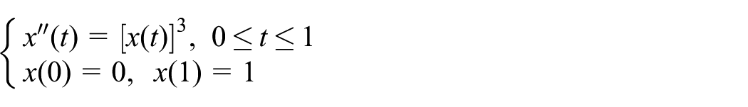
Example 2

As the second example, consider the following integral equation

u (t) = \sin (\frac{π}{2} t) - \frac{11 t}{6} + \int_{0}^{1} 4 π ty \sin (π y) {[u (y)]}^{4} dy

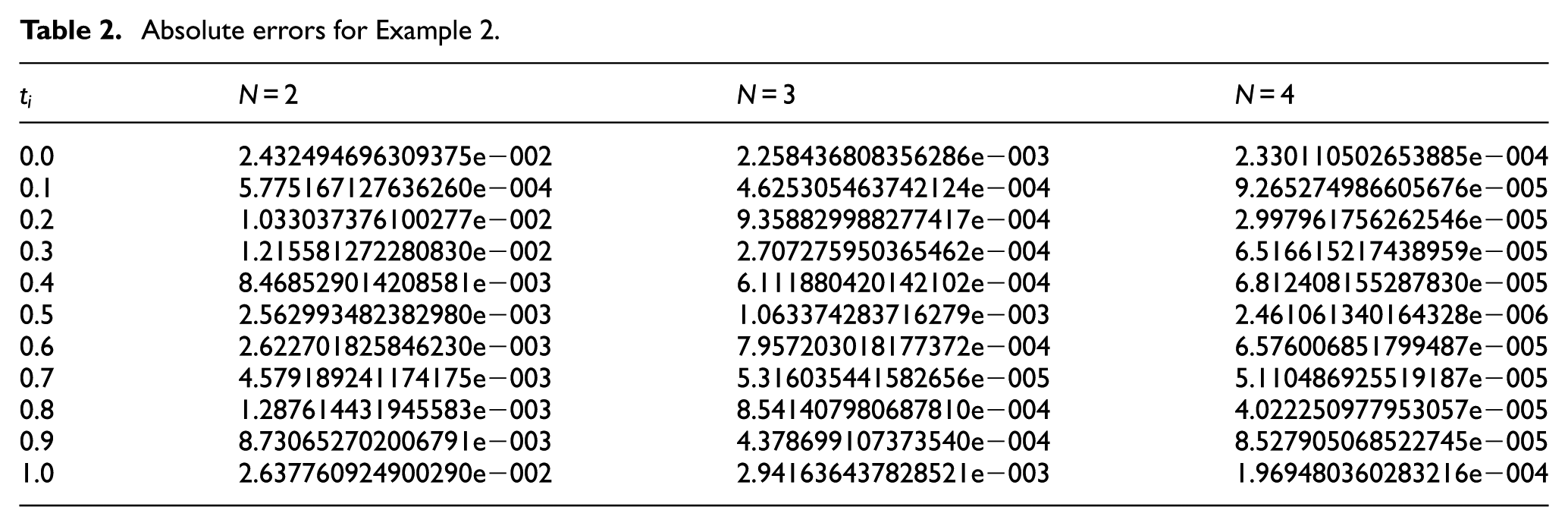
with exact solution $u (t) = \sin (\frac{π}{2} t)$ . Table 2 and Figure 2 show the numerical results for Example 2.

Table 2.

Absolute errors for Example 2.

$t_{i}$	N = 2	N = 3	N = 4
0.0	2.432494696309375e−002	2.258436808356286e−003	2.330110502653885e−004
0.1	5.775167127636260e−004	4.625305463742124e−004	9.265274986605676e−005
0.2	1.033037376100277e−002	9.358829988277417e−004	2.997961756262546e−005
0.3	1.215581272280830e−002	2.707275950365462e−004	6.516615217438959e−005
0.4	8.468529014208581e−003	6.111880420142102e−004	6.812408155287830e−005
0.5	2.562993482382980e−003	1.063374283716279e−003	2.461061340164328e−006
0.6	2.622701825846230e−003	7.957203018177372e−004	6.576006851799487e−005
0.7	4.579189241174175e−003	5.316035441582656e−005	5.110486925519187e−005
0.8	1.287614431945583e−003	8.541407980687810e−004	4.022250977953057e−005
0.9	8.730652702006791e−003	4.378699107373540e−004	8.527905068522745e−005
1.0	2.637760924900290e−002	2.941636437828521e−003	1.969480360283216e−004

Figure 2.

Comparison plot of exact and approximation solution of Example 2, for N = 2, 3, and 4.

Example 3 (application to the BVP functional differential equations)

One of the important problems in science and engineering is a BVP for functional differential equations which is investigated by numerous researchers.^54,55 This problem can be converted, using Green’s function technique, into a Hammerstein integral equation.^56–59 Here, we consider an example of this problem as an application of our methods.

Consider the two-point BVP

{\begin{matrix} x ″ (t) = [x (t)]^{3}, 0 \leq t \leq 1 \\ x (0) = 0, \begin{matrix} x (1) = 1 \end{matrix} \end{matrix}

This BVP is equivalent with the following Hammerstein integral equation

u (t) - \int_{0}^{1} K (t, y) {[u (y)]}^{3} dy = t, \begin{matrix} t \in [0, 1] \end{matrix}

where

K (t, y) = {\begin{matrix} - y (1 - t), y \leq t \\ - t (1 - y), y \geq t \end{matrix}

is the Green function.

To solve this problem, we applied three methods.

Method I (using the shifted Chebyshev polynomials and Galerkin methods with approach of operational vector)

In this approach, first, we use the shifted Chebyshev polynomials as $Ψ (y) = [ψ_{1} (y), ψ_{2} (y), \dots, ψ_{N} (y)]^{T}$ .³³ Then, we approximate $[u (y)]^{m}$ as follows:

[u (y)]^{m} = [U^{T} Ψ (y)]^{m} = U_{m}^{* T} Ψ (y)

where $U_{m}^{* T}$ is a column vector, whose elements are nonlinear combinations of the elements of the vector U. $U_{m}^{* T}$ is called the operational vector of the mth power of the function $u (y)$ (see equation (4.2) in Mahmoudi³³).

Method II (using the shifted Chebyshev polynomials and Galerkin methods with the approach of the equivalent equation)

In this approach, first, by using the shifted Chebyshev polynomials, we obtain^13,15,34

u (y) \approx \sum_{i = 0}^{N} c_{i} b_{i} (t)

Then, we approximate $[u (y)]^{m}$ as follows

[u (y)]^{m} = ψ (y, u (y)) = ψ (y, \sum_{i = 1}^{n} c_{i} \int_{a}^{b} K (t, y) b_{i} (y) dy + f (y))

Method II (present method—Algorithm 1)

After testing these three methods on the mentioned example, we see that where the absolute errors in all three methods for Example 3 with different N, t is almost the same; however, the computational costs in these methods are different. In Table 3, we report the total CPU time for the corresponding methods.

Table 3.

CPU time for Example 3.

Method	N = 4	N = 8	N = 16	N = 32
Method I	4.6137	9.7566	21.2418	42.334
Method II	3.2564	7.9783	15.3990	27.6430
Present method	1.9705	5.0370	9.0375	18.2325

From the results, we can see that the present method works better than the other two existing approaches.

Conclusion

In this article, we have proposed a new algorithmic method for the solution of Hammerstein integral equation. This method is very simple to apply and to make an algorithm. Numerical examples are given to further compare the approximation solution of this method with the exact solution, which shows the feasibility and effectiveness of the method for solving Hammerstein integral equation.

Footnotes

Academic Editor: Yi Wang

Declaration of conflicting interests

The author(s) declared no potential conflicts of interest with respect to the research, authorship, and/or publication of this article.

Funding

The author(s) received no financial support for the research, authorship, and/or publication of this article.

References

Corduneanu

Integral equations and applications. New York: Cambridge University Press, 1973.

Burton

TA.

Volterra integral and differential equations. New York: Academic Press, 1983.

Lovitt

WW.

Linear integral equations. New York: Dover, 1950.

Agarwal

O’Regan

Wong

PJY

. Positive solutions of differential, difference and integral equations. Dordrecht: Kluwer Academic, 1999.

Ladopoulos

EG.

Singular integral equations linear and non-linear theory and its applications in science and engineering. Berlin; Heidelberg: Springer, 2000.

Cardinali

Papageorgiou

NS.

Hammerstein integral inclusions in reflexive Banach spaces. American Math Soc 1999; 127: 95–103.

Atkinson

KE.

The numerical solution of integral equations of the second kind. Cambridge: Cambridge University Press, 1997.

Hammerstein

Nichtlineare integralgleichungen nebst anwendungen. Acta Math 1930; 54: 117–176.

Tricomi

FG.

Integral equations. Mineola, NY: Dover Publications, 1982.

10.

Kumar

Sloan

IH.

A new collocation-type method for Hammerstein integral equations. Math Comput 1987; 48: 123–129.

11.

Brunner

Implicitly linear collection methods for nonlinear Volterra equations. Appl Numer Math 1992; 9: 35–47.

12.

Guoqiang

Asymptotic error expansion of a collection type method for Volterra–Hammerstein integral equations. Appl Numer Math 1993; 13: 357–369.

13.

Elnagar

Kazemi

Chebyshev spectral solution of nonlinear Volterra–Hammerstein integral equations. J Comput Appl Math 1996; 76: 147–158.

14.

Hernandez

Rubio

Ezquerro

JA.

Secant-like methods for solving nonlinear integral equations of the Hammerstein type. J Comput Appl Math 2000; 115: 245–254.

15.

Kaneko

Noren

Novaprateep

Wavelet applications to the Petrov–Galerkin method for Hammerstein equations. Appl Numer Math 2003; 45: 255–273.

16.

Contea

Prete

ID.

Fast collocation methods for Volterra integral equations of convolution type. J Comput Appl Math 2006; 196: 652–663.

17.

Dehghan

Saadatmandi

A tau method for the one-dimensional parabolic inverse problem subject to temperature overspecification. Comput Math Appl 2006; 52: 933–940.

18.

Doha

Bhrawy

AH.

Efficient spectral-Galerkin algorithms for direct solution of fourth-order differential equations using Jacobi polynomials. Appl Numer Math 2008; 58: 1224–1244.

19.

Bhrawy

Alofi

AS.

A Jacobi-Gauss collocation method for solving nonlinear Lane-Emden type equations. Commun Nonlinear Sci 2012; 17: 62–70.

20.

Bhrawy

AH.

A Jacobi–Gauss–Lobatto collocation method for solving generalized Fitzhugh–Nagumo equation with time-dependent coefficients. Appl Math Comput 2013; 222: 255–264.

21.

Bhrawy

AH.

An efficient Jacobi pseudospectral approximation for nonlinear complex generalized Zakharov system. Appl Math Comput 2014; 247: 30–46.

22.

Sommariva

A fast Nyström–Broyden solver by Chebyshev compression. Numer Algorithms 2005; 38: 47–60.

23.

Cheng

Huang

Extrapolation algorithms for solving nonlinear boundary integral equations by mechanical quadrature methods. Numer Algorithms 2011; 58: 45–554.

24.

Cai

A fast Fourier-Galerkin method for solving singular boundary integral equations. SIAM J Numer Anal 2008; 46: 965–1984.

25.

Alipanah

Dehghan

Numerical solution of the nonlinear Fredholm integral equations by positive definite functions. Appl Math Comput 2007; 190: 754–1761.

26.

Jiang

Fast Fourier-Galerkin methods for solving singular boundary integral equations: numerical integration and precondition. J Comput Appl Math 2010; 234: 792–2807.

27.

Bhrawy

Abdelkawy

Tenreiro Machado

. Legendre–Gauss–Lobatto collocation method for solving multi- dimensional Fredholm integral equations. Comput Math Appl. Epub ahead of print 28 April 2016. DOI: 10.1016/j.camwa.2016.04.011.

28.

Bhrawy

Tohidi

Soleymani

A new Bernoulli matrix method for solving high-order linear and nonlinear Fredholm integro-differential equations with piecewise intervals. Appl Math Comput 2012; 219: 482–497.

29.

Chen

Wang

Fast Fourier-Galerkin methods for nonlinear boundary integral equations. J Sci Comput 2013; 56: 94–514.

30.

Hashemizadeh

Rostami

Numerical solution of Hammerstein integral equations of mixed type using the Sinc-collocation method. J Comput Appl Math 2015; 279: 31–39.

31.

Das

Gnaneshwar

Guangqing Long

Discrete Legendre spectral projection methods for Fredholm–Hammerstein integral equations. J Comput Appl Math 2015; 278: 293–305.

32.

Jang

G-W

Kim

Choi

KK.

Remesh-free shape optimization using the wavelet-Galerkin method. Int J Solids Struct 2004; 41: 6465–6483.

33.

Mahmoudi

Wavelet Galerkin method for numerical solution of nonlinear integral equation. Appl Math Comput 2005; 167: 1119–1129.

34.

Maleknejad

Karami

Rabbani

Using the Petrov–Galerkin elements for solving Hammerstein integral equations. Appl Math Comput 2006; 172: 831–845.

35.

Xiao

J-Y

Wen

L-H

Zhang

Solving second kind Fredholm integral equations by periodic wavelet Galerkin method. Appl Math Comput 2006; 175: 08–518.

36.

Lepik

. Haar wavelet method for nonlinear integro-differential equations. Appl Math Comput 2006; 176: 324–333.

37.

Maleknejad

Lotfi

Rostami

Numerical computational method in solving Fredholm integral equations of the second kind by using Coifman wavelet. Appl Math Comput 2007; 186: 212–218.

38.

Ordokhani

Razzaghi

Solution of nonlinear Volterra–Fredholm–Hammerstein integral equations via a collocation method and rationalized Haar functions. Appl Math Lett 2008; 21: 4–9.

39.

Babolian

Shahsavaran

Numerical solution of nonlinear Fredholm integral equations of the second kind using Haar wavelets. J Comput Appl Math 2009; 225: 87–95.

40.

Aziz

Siraj-ul-Islam . New algorithms for the numerical solution of nonlinear Fredholm and Volterra integral equations using Haar wavelets. J Comput Appl Math 2013; 239: 333–345.

41.

Najafi

Aminikhah

Edalatpanahand

SA.

Linear Legendre multi-wavelets method for solving systems of Fredholm integral equations. Math Rep 2016; 18: 41–50.

42.

Abbasbandy

Numerical solutions of the integral equations: homotopy perturbation method and Adomian decomposition method. Appl Math Comput 2006; 173: 493–500.

43.

Dong

Chen

Jiang

A modified homotopy perturbation method for solving the nonlinear mixed Volterra–Fredholm integral equation. J Comput Appl Math 2013; 239: 359–366.

44.

Abdou

El-Borai

El-Kojok

MM.

Toeplitz matrix method and nonlinear integral equation of Hammerstein type. J Comput Appl Math 2009; 223: 65–776.

45.

Maleknejad

Lotfi

Numerical expansion method for solving integral equation by interpolation and Gauss quadrature rules. Appl Math Comput 2005; 168: 111–124.

46.

Bica

Curila

About a numerical method of successive interpolations for functional Hammerstein integral equations. J Comput Appl Math 2012; 236: 2005–2024.

47.

Bazm

Bernoulli polynomials for the numerical solution of some classes of linear and nonlinear integral equations. J Comput Appl Math 2015; 275: 44–60.

48.

Atkinson

Han

Theoretical numerical analysis: a functional analysis framework (vol. 39, Texts in Applied Mathematics). New York: Springer, 2007.

49.

Chihara

TS.

An introduction to orthogonal polynomials. New York: Gordon & Breach Science Publisher, 1978.

50.

Mason

Handscomb

DC.

Chebyshev polynomials. Boca Raton, FL: CRC Press, 2003.

51.

Synder

MA.

Chebyshev methods in numerical approximation. London: Prentice Hall, 1966, p. 40.

52.

Doha

Bhrawy

Ezz-Eldien

SS.

Efficient Chebyshev spectral methods for solving multi-term fractional orders differential equations. Appl Math Model 2011; 35: 5662–5672.

53.

Bhrawy

Alofi

AS.

The operational matrix of fractional integration for shifted Chebyshev polynomials. Appl Math Lett 2013; 26: 25–31.

54.

Yao

Solvability of a fourth-order beam equation with all-order derivatives. Southeast Asian Bull Math 2008; 32: 563–571.

55.

Chen

. Fast multilevel augmentation methods for nonlinear boundary integral equations. SIAM J Numer Anal 2011; 49: 2231–2255.

56.

Madbouly

McGhee

Roach

GF.

Adomian’s method for Hammerstein integral equations arising from chemical reactor theory. Appl Math Comput 2001; 117: 241–249.

57.

Jankowski

Positive solutions for fourth-order differential equations with deviating arguments and integral boundary conditions. Nonlinear Anal: Theor 2010; 73: 1289–1299.

58.

Bica

AM.

The numerical method of successive interpolations for Fredholm functional integral equations. Numer Algorithms 2011; 58: 351–377.

59.

Infante

Paolamaria

Mattia Tenuta

Existence and localization of positive solutions for a nonlocal BVP arising in chemical reactor theory. Commun Nonlinear Sci 2014; 19: 2245–2251.

An efficient algorithmic method to solve Hammerstein integral equations and application to a functional differential equation

Abstract

Keywords

Introduction

Solving the Hammerstein integral equations

Properties of shifted Chebyshev polynomials

Galerkin method

Main results

Algorithm 1

Illustrative examples

Example 1

Example 2

Example 3 (application to the BVP functional differential equations)

Method I (using the shifted Chebyshev polynomials and Galerkin methods with approach of operational vector)

Method II (using the shifted Chebyshev polynomials and Galerkin methods with the approach of the equivalent equation)

Method II (present method—Algorithm 1)

Conclusion

Footnotes

Declaration of conflicting interests

Funding

References