
Abstract
Tire wear quantity and difference is one of the main points that affect the intension of tire road print feature and is under a tight link not only with tire road friction energy but also with vehicle dynamics. The proposed methodology aims to provide a mathematical method to analyze tire marks’ feature for prediction the vehicle operating status in pro- and post-crash phases. The kinetic sliding friction coefficient considering the road effect is simplified with the new real contact area model. After, a simplified 9 degrees of freedom vehicle dynamics model by coupling the tire dynamic model is set up, and the effectiveness of the model is evaluated with vehicle stability measurement equipment. Furthermore, a theoretical model of tire wear quantity and difference as a function of road properties and vehicle dynamics is set up combined with vehicle–road coupling algorithm, and important parameters (e.g. vehicle speed, steering angle, braking force, and road feature) are analyzed to assess the tire wear quantity and difference feature when the vehicle is in unsteady condition. Results show that vehicle speed, braking force, and road surface feature have a significant impact to tire wear quantity and difference, the right rear exhibits a fluctuation and the tire wear quantity and difference between rear axle and the right side is obvious, and lay a strong foundation for tire road print analysis.
Keywords
Introduction
Accident reconstruction is commonly found on police accident scene reports, on witness testimonials, and especially on traces discovered at the accident scene and vehicles involved in the accident. Even with the increasing use of event data recorders, tire marks are still remaining as a major element of gaining reliable information about vehicle trajectories, initial velocities, and vehicle dynamics during pro- and post-crash phases of an accident. During this phase, the amount of tire tread wear lead the intensity of tire marks and the amount distribute lead tire marks explicit–inexplicit characteristic, as shown in Figure 1, we call this as tire wear quantity and difference (TWQD). In particular, the connection between the emergence of tire marks, road properties, and vehicle dynamic parameters is not well characterized.

The explicit–inexplicit feature of tire marks.
Tire wear has long been a research topic with the pressing need from civil needs, and TWQD is considered the main reason impacting the tire marks’ feature. From the reasonable point of view, tire materials, vehicle dynamics, and road properties are three core factors which impact the tire wear.1,2 In nature, the tire wear is caused by the sliding between the tire tread and the road and depends on frictional work developed by tire–road contact (level and vertical).2–4 In recent years, a dynamic sliding friction is proposed to analyze the mechanisms of interaction between tire and road surface,5–7 which can compute the frictional work when tire–road is in a sliding condition. Meantime, in order to obtain the tire wear quantity, the numerical calculation 8 from the energy aspect and the finite element analysis method 9 has been proposed. For example, Braghin et al. 10 have predicted the global tire wear qualitatively using a mathematical model with an empirical local friction and wear correlation.
Some literatures indicated that the rough-road properties have a significant impact to the friction coefficient. 11 Using dynamic sliding friction and vehicle dynamic model, researchers can analyze the road properties to the vehicle dynamics, four wheels’ tire forces, and difference under different conditions. 12 In a recent study, an approach combined with vehicle dynamics and qualitative formula for tire wear is proposed to estimate the tire wear quantity during longitudinal and cornering maneuvers. 13 However, few research attempts have been made to investigate TWQD between four wheels with consideration of the vehicle dynamics based on road properties.
In this study, a theoretical model describing the TWQD is proposed using the vehicle–road coupling algorithm, and this model is the function of road properties, tire feature, and vehicle dynamics. The simplified kinetic friction model is utilized to evaluate the rough-road properties and tire tread feature. By coupling the sliding friction model, tire model, and a simplified 9 degrees of freedom (DOF) vehicle dynamic model, the road features’ effect on tire road friction dissipation energy and tire wear can be computed qualitatively based on vehicle dynamic parameters. After validation, the impact of vehicle dynamics, road properties to TWQD, is considered in this model. Additionally, some expressions found in the literature allow the researcher to predict TWQD using simplified models and these standard expressions for prediction of the vehicle operating status in accident reconstruction.
The construct of TWQD coupling system
The objective of this research is to analyze the TWQD with respect to three main categories of influencing factors, such as tire–road friction, tire–road dynamics, and vehicle dynamics, as shown in Figure 2.

Cause and effect chain of TWQD.
The basic approach of TWQD analysis involves the development of equations for road properties and vehicle dynamics. The category “tire–road friction” describes the friction between tire and rough road. By fitting this kinetic sliding friction coefficient, the effect of road properties and tire feature to tire dynamic is achieved. The category “vehicle dynamics” could explore the four wheels’ tire forces and difference under unsteady condition impacted by vehicle dynamics, such as vehicle speed, braking force, and steer angle. After coupling, the vehicle dynamics and tire–road dynamics, we get the vehicle–road-coupled model and could obtain four wheels’ tire force and difference under vehicle unsteady condition. Finally, TWQD will be calculated as a function of given road properties, tire feature, and vehicle dynamics combined with the wear quantity method. In the following sections, the models of these categories are explained in detail.
Modeling and validation of the simplified kinetic rubber sliding friction coefficient
The simplified real contact area model
Understanding the contact mechanism is imperative to study the friction performance between the tire and rough pavement. In general case, the micro-bulge on the rough pavement is irregular and follows the Gauss distribution, 7 and accurate calculations are rather difficult because a number of small contacting asperities within an apparent contact region can easily deform because of their low elasticity. In nature, when the tire contacts with the rough road, it is not contacted every region and the real contact area is the total of the micro-contact region. 11 For one micro-contact, supposing the curvature of spheres is dependent on the asperity height and summits of very large heights behave as perfectly spherical, 7 the contact area model can be further simplified. The contact mechanism is shown in Figure 3.

The simplified contact mechanism.
After being simplified, the probability density distribution function of the micro-convex body in the contact area

Then, the normal force

In range of vertical load, the contact between tire and the micro-bulge is in the large separation and the contact is at the Hertz theory state,5,6 then the real contact area is as follows

Meantime, the relationship between the real contact area and the normal force is simplified as follows

The simplified kinetic sliding friction coefficient
The modeling of kinetic sliding friction coefficient on self-affine surfaces has been treated by several authors based on the hysteretic energy losses arising from the rubber deformation by surface asperities. 14 After appropriate simplification of the real contact area, combined with the simplification of the viscoelastic energy loss, the kinetic sliding friction coefficient calculation also has two components: the hysteretic friction coefficient and the adhesion friction coefficient. 12 Here, the friction coefficient depends on the sliding velocity, normal force, tire feature, and road self-affine characteristics; the calculation can be simplified as follows
The surface roughness power spectrum

Here

Verification of friction coefficient
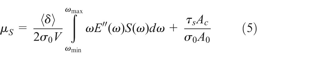
A rather simple but useful kinetic sliding friction coefficient of Savkoor 15 for the dynamic application 10 is employed to validate the proposed simplifying dynamic sliding friction coefficient; the function is as follows

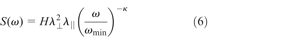
As the most commonly used in vehicle dynamic analysis, it can characterize the effect of sliding velocity, the normal force. To eliminate the effect of contact pressure, the comparison between two models is conducted at 0.3 MPa. The Savkoor fitting parameters are listed in Table 1, the road self-affine parameters are listed in Table 2, and the comparison results are shown in Figure 4.
The fitting parameters of Savkoor.
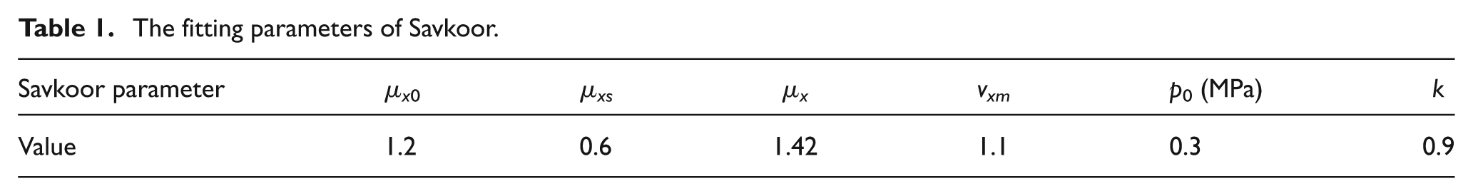
Road self-affine parameter.

Comparison results between two kinetic sliding friction coefficients.
From the comparison results in Figure 4, the discrepancy between Savkoor and simplified kinetic sliding friction coefficient is less than 3% and the validation of the simplified sliding friction model is verified. With the utilization of this simplified sliding friction coefficient, the impact of road properties and tire feature to the kinetic sliding friction coefficient and tire dynamics can be well characterized and illustrated.
Power function of TWQD
The proposed mathematic method is to evaluate the TWQD based on road properties, tire feature and vehicle dynamics. So, a qualitative formulation for tire wear quantity is derived for vehicle dynamics responses considering the road effect to provide the vehicle–road coupling dynamic response in the subsequent sections. First, tire slip quantities that define the frictional work between the tire and road surface is introduced.
Definition of the tire slide quantities
When imposed on the braking torque, the tire is working at sliding condition and the slip ratio is used to illustrate the proportion of the sliding part. Figure 5 shows a diagram of longitudinal and lateral tire slip quantities that are introduced in the SAE axis system.

Diagram of the vertical contact pressure and tire slip quantities.
As shown in Figure 5, the longitudinal slide velocity

Similarly, the lateral slip velocity of the tire is equal to the lateral speed at the point of contact with the road plane; that is

The longitudinal and lateral slip ratios

and

Definition of the friction dissipation energy and road feature
The tire wear quantity is corresponding to the friction energy rates. The tire friction energy rates produced in each wheel are computed by the dynamic frictional rolling analysis of tire model. According to the law of energy conservation, the friction energy rates of each direction under sliding condition are as follows


Considering the tire dynamic characteristic and fitting the friction coefficient, the Fiala nonlinear tire dimensionless model is employed 16 to characterize the force within the tread contact area. The formula can be written as follows

Here

Qualitative formulation for TWQD
Previous study has been proved that the wear quantity and the friction dissipation energy have a proportional relationship. 10 Therefore, this simple model 17 is employed here to predict the quantity of wear. The expression is as follows

The fitting parameters of rubber wear and friction power of tire 17 obtained from tests are shown in Table 3.
The fitting parameters of rubber wear quantity.

The relationship between wear quantity and wear energy under different conditions is shown in Figure 6.
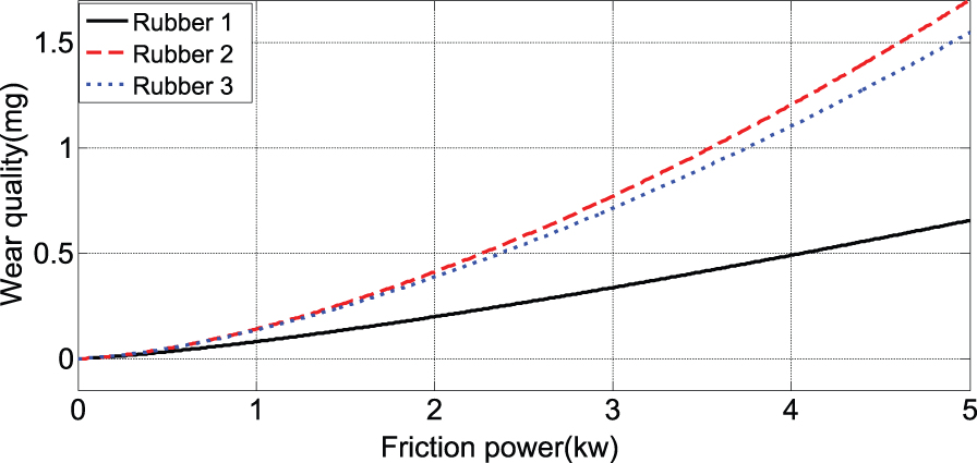
Relationship of the wear quantity and friction power.
Theoretically speaking, the wear quantity refers to the total friction dissipation energy, and the expressions of each tire wear quantity are as follows

So, the wear quantity difference between front tires and rear tire can be written as follows


Similarly, the wear quantity difference between right and left sides can be evaluated in the same way. Therefore, equations (20)–(22) together serve as the tire wear quantity model which may be used to describe TWQD under unsteady state from braking and cornering maneuvers exerted until the vehicle stopped. To computerize TWQD, the product of longitudinal and lateral forces at unsteady state should be obtained first, which is the function of the normal force and the vehicle dynamics.
Simplified vehicle model for evaluation of nonlinear dynamics
Vehicle dynamic model
An accurate and realistic vehicle model is essential for the effective vehicle dynamic analysis. Many different vehicle models have been developed and the assumptions made in their development depend on their application. 14 In order to better represent the vehicle lateral and yaw dynamics as well as coupling of yaw–roll motion due to the transient lateral load transfer 18 during extreme maneuvers, a 9 DOF model is valid for applications which do not involve wheel lift-off. 14 So, the selection of 9 DOF vehicle models is advantageous. The nonlinear model can be derived from the summation of forces and moments in the bicycle model shown in Figure 7.
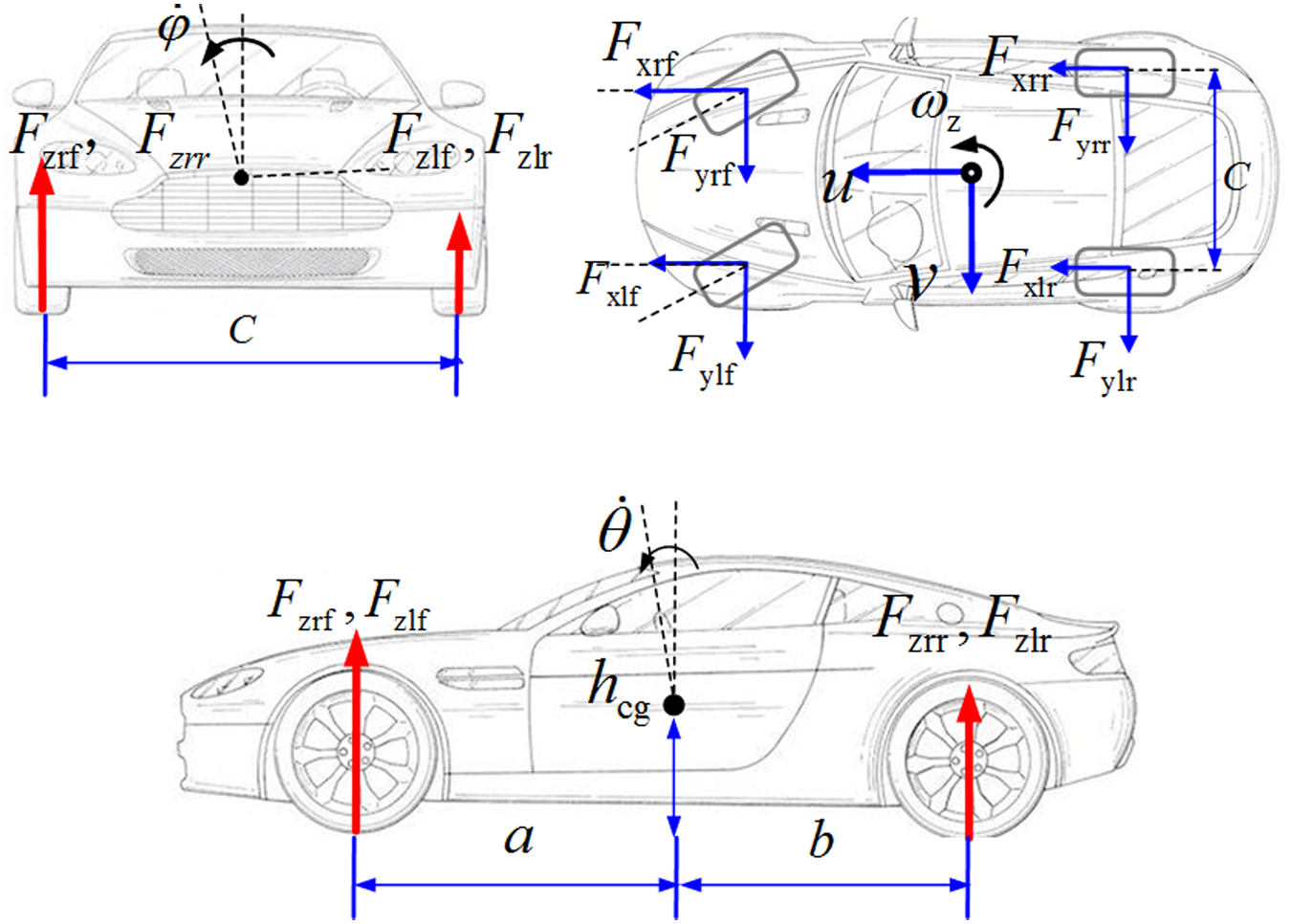
Vehicle dynamic model with 9 DOFs.
According to the rigid body kinematics and dynamics of principle, the equations of motion for 5 DOFs of the sprung mass model can be derived from the direct application of Newton’s laws for the system as follows


The normal forces at the four tires are determined as follows


Verification of vehicle dynamic model
The yaw rate, as the main dynamic parameters of the vehicle, is employed to validate the 9 DOF vehicle dynamics model using the stability measurement system with the combined steering–braking maneuver at 25 km/h initial velocities. The steering angle is fixed at −1 rad, the braking torque is 600 and 400 N m for front and rear wheels, respectively. The vehicle stability measurement system consists VBOX (data acquisition system based on Global Positioning System (GPS)), gyroscope (measuring the vehicle dynamic parameters), steering angle measurement, power, data acquisition module, computer, and so on, as shown in Figure 8. The vehicle structure parameters are determined in Table 4, and the verification results are presented in Figure 9.

Measurement system of vehicle stability.
The vehicle structural parameters.


Verification of the proposed vehicle dynamics: (a) yaw rate and (b) braking speed.
From Figure 9, it is clearly that the simulations of the vehicle dynamics model approach a fairly agree with the experimental results at response time, change trends, and maximum value. The maximum yaw rate reached at about 0.08 rad/s and illustrated that the vehicle is in the stable state. So, the 9 DOF vehicle dynamics models can effectively analyze the vehicle unsteady dynamics and provide the longitudinal, lateral, and normal force to analyze TWQD reliability.
Qualitative analysis and discussion
It is difficult to evaluate TWQD in random conditions because there are too many variations in parameter uncertainties owing to various excitations. Therefore, some parameters were varied in order to determine their effects by modifying the single parameters at one time. For the vehicle dynamics, such as vehicle speed, braking force, and steering angle are the inputs to analyze the desired dynamic responses. For the road effect, the parameters of kinetic sliding friction coefficient could be changed and evaluated. The road self-affine parameters are shown in Table 2, the parameters of rubber 1 in Table 3 are chosen, and the vehicle structural parameters are listed in Table 4.
The impact of vehicle dynamics to TWQD
For dynamic vehicle dynamic responses, the vehicle speeds, braking force, and steering angle have been determined.
Vehicle speed effect to TWQD
On dry asphalt road, the steering angle is −1.5 rad, the front and rear braking torques are fixed at 700 and 450 N, respectively. Then, we can obtain the effect of vehicle speed to TWQD at three alternatives: 15, 20, and 25 m/s. The comparison results are shown in Figures 10 and 11.

The impact of vehicle speed to wear quantity of four tires: wear quantity of (a) right-front tires, (b) left-front tires, (c) right-rear tires, and (d) left-rear tires.

The impact of vehicle speed to wear quantity difference between four tires: wear quantity difference of (a) the front axle tires, (b) the rear axle tires, (c) the right-side tires, and (d) the left-side tires.
The whole braking process could be divided into three phases: initial braking phase (0–1 s), post-braking phase (1–2 s), and end-braking phase (2s-stopping). It is obvious that the total braking process has a significant impact to TWQD in initial braking phase and post-braking phases.
As shown in Figure 10, the maximum wear quantity of front and rear axis are 0.08, 0.12, 0.25 mg and 0.02, 0.035, 0.08 mg, respectively, and indicate that the tire wear degree of the front axis is more serious than rear axis. Moreover, the simulation results also show a nonlinear proportion between tire wear quantity and vehicle speed. Exceptionally, the wear quantity of right-rear wheel exhibits a fluctuation when the vehicle speed is 25 m/s and speculation leading the tire marks different intensity and is continuous, but the normal force in this wheel is relatively smaller in this condition.
When comparing four simulation results (tire wear difference with braking time) at the same condition together, we can also find that the tire wear quantity difference is larger with the vehicle speed increase, as shown in Figure 11. When the vehicle speed is 25 m/s, the biggest differences of wear quantity are 0.006, 0.03, 0.102, and 0.108 mg corresponding to front axle tires, rear axle tires, right-side tires, and left-side tires, respectively. It is obvious that rear axle and two-side wheel have large tire wear quantity difference. Relatively speaking, the tire wear quantity of right rear (minimum vertical load) is highest in rear axle. The right-side tire wear quantity difference could lead the tire marks intensity difference.
Braking force effect to TWQD
On dry asphalt road, the steering angle is −1.5 rad, and the vehicle speed is fixed at 20 m/s. Then, we can obtain the effect of braking force to TWQD at three alternatives’ braking force: 600–350 N, 700–450 N, and 800–550 N, respectively. The comparison results are shown in Figures 12 and 13.
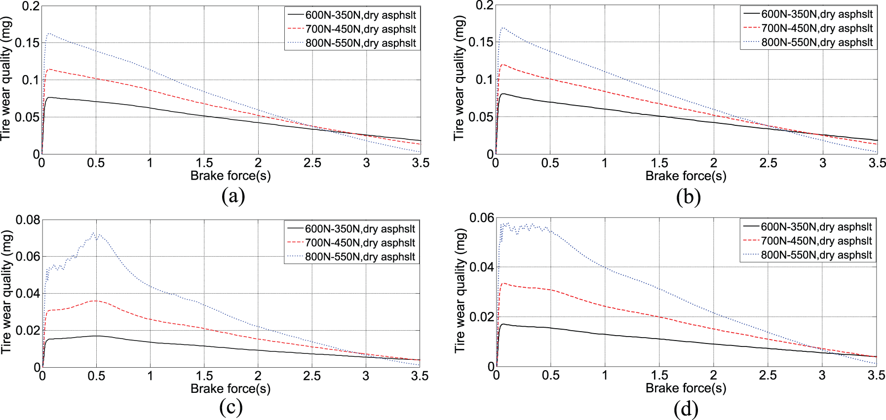
The impact of braking force to wear quantity of four tires: wear quantity of (a) right-front tire, (b) left-front tire, (c) right-rear tire, and (d) left-rear tire.
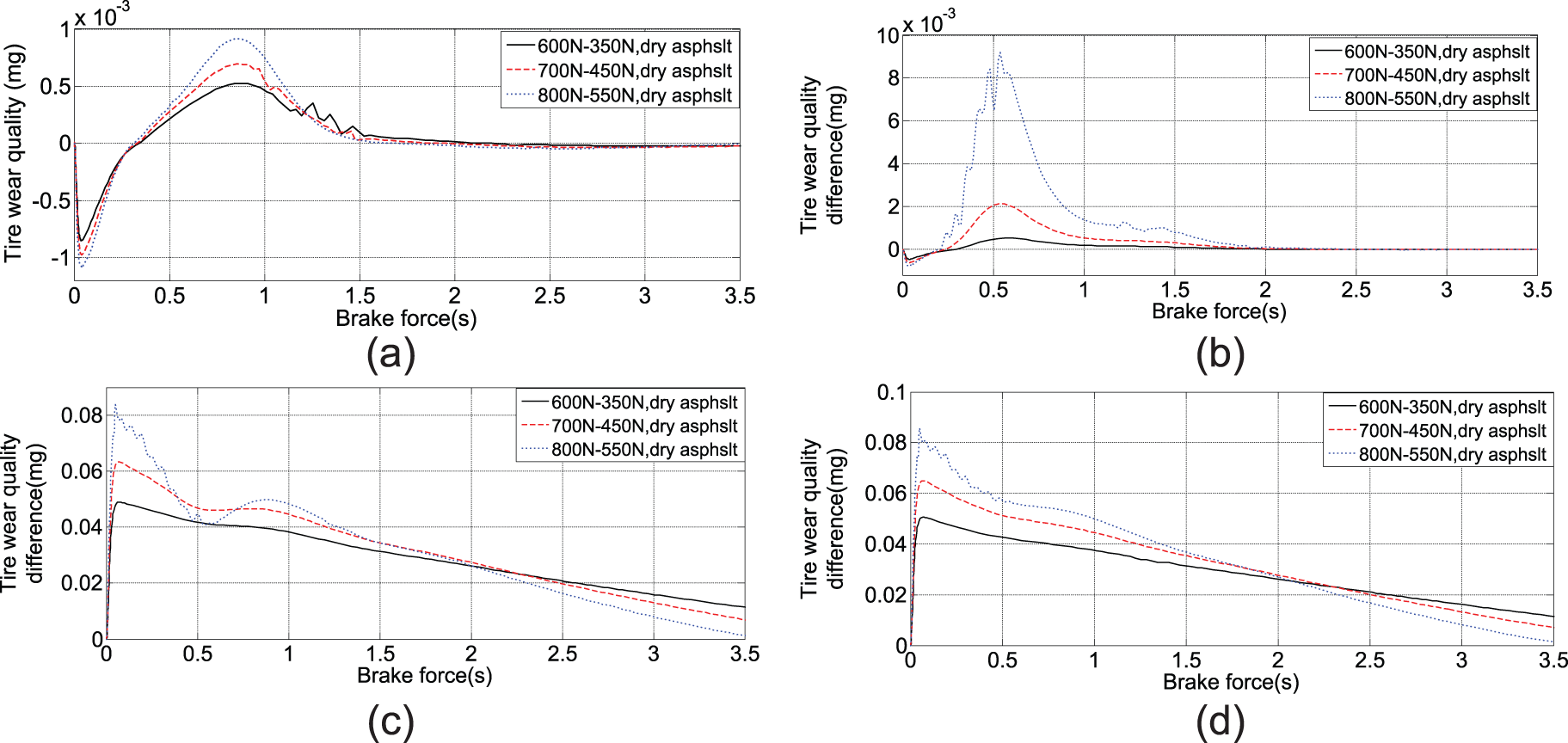
The impact of braking force to wear quantity difference between four tires: wear quantity difference of (a) the front axle tires, (b) the rear axle tires, (c) the right-side tires, and (d) of the left-side tires.
Steering angle effect to TWQD
On dry asphalt road, the vehicle speed is fixed at 20 m/s, the front and rear braking torques are fixed at 700 and 450 N. Then, we can obtain the effect of steering angle to TWQD at three steering angles: −1, −1.5, and −2 rad. The comparison results are shown in Figures 14 and 15.

The impact of steering angle to wear quantity of four tires: wear quantity of (a) right-front tire, (b) left-front tire. (c) right-rear tire, and (d) left-rear tire.

The impact of steering angle to wear quantity difference between four tires: wear quantity difference of (a) the front axle tires, (b) the rear axle tires, (c) right-side tires, and (d) the left-side tires.
Figures 12 and 13 show that the impact of braking force to TWQD is also significant and similar to vehicle speed, but the total impact is smaller. The maximum wear quantities are 0.16, 0.17, 0.07, and 0.06 mg corresponding to right front, left front, right rear, and left rear, respectively, and the wear quantity differences are 0.0008, 0.09, 0.08, and 0.08 mg corresponding to the front axle, rear axle, right side, and left side, respectively. However, compared to the effect of braking force and vehicle speed, the impact of steering angle is weak and can be neglected, as shown in Figures 14 and 15.
Compared with Figures 12 and 14, Figure 10 illustrates that the vehicle speed affects the tire wear quantity severely; therefore, the vehicle speed is a dominate parameter impacting TWQD. Based on the analysis, an interesting result is that the smaller normal force side has higher wear quantity. TWQD has an inverse relationship with the lateral force and is a combined result of many factors such as vehicle speed, steering angle, and braking force.
The impact of road properties to TWQD
In this condition, tire rubber 1 parameter is utilized. In this section, the steering angle is set at −1.5 rad, the vehicle speed is fixed at 20 m/s, the front and rear wheel braking torques are 800 and 550 N, respectively. Simulation results of TWQD are presented in Figures 16 and 17, respectively.

The impact of road surface features to wear quantity of four tires: wear quantity of (a) right-front tire, (b) left-front tire, (c) right-rear tire, and (d) left-rear tire.

The impact of road surface features to wear quantity difference between four tires: wear quantity difference of (a) the front axle tires, (b) the rear axle tires, (c) the right-side tires, and (d) the left-side tires.
Figures 16 and 17 show that the front tire wear quantity is higher and the maximum value is about 0.2 mg, but there is no significant difference between different road properties. The influence of road properties on the front and rear axle wheel in the first period is significantly. The tire wear quantity on dry asphalt is least and on wet asphalt is higher. Because the dry asphalt has a higher kinetic sliding friction coefficient, so we can surmise that the TWQD have an inverse relationship with kinetic sliding friction coefficient.
The wear quantity difference between four tires on different roads is not obvious, and the maximum values are 0.06, 0.08, and 0.08 mg corresponding to rear axle, right side, and left side, respectively. But, the TWQD in wet asphalt (lower kinetic sliding friction coefficient) exhibits the fluctuation, the probable reason is that the vehicle already transits to unsteady state for the tire force provided by pavement which is not bigger enough to maintain the vehicle stability. In this condition, the tire has a severe wear and more complex factors contribute to TWQD and need a further study.
Conclusion
In this article, a theoretical model describing TWQD as a function of road properties, tire feature, and vehicle dynamics is established using the vehicle–road coupling algorithm. The kinetic sliding friction model is utilized to evaluate the road properties, and a simplified 9 DOF vehicle dynamics model is developed to evaluate the vehicle dynamics. The vehicle stability measurement system is set up and the effectiveness of model is evaluated. Simulation results show TWQD is a combined result of many factors such as vehicle speed, steering angle and braking force, road properties, and tire feature. Three clear conclusions can be observed:
The vehicle speed is a dominating parameter impacting TWQD, and the total impact of braking force is smaller and the impact of steering angle is weaker and can be neglected.
The right-rear tire wear exhibits a fluctuation and the wear quantity difference between rear axle and the right side is obvious.
TWQD has an inverse relationship with the lateral force and kinetic sliding friction coefficient.
The proposed methodology aims to provide a mathematic method to predict the tire marks’ features of accident vehicle for prediction the vehicle operating status in accident reconstruction.
Footnotes
Appendix 1
Academic Editor: Yongjun Shen
Declaration of conflicting interests
The author(s) declared no potential conflicts of interest with respect to the research, authorship, and/or publication of this article.
Funding
The author(s) disclosed receipt of the following financial support for the research, authorship, and/or publication of this article: This research was supported partly by the outstanding talent financing plan of Beijing Municipal Party Committee Organization Department (no. 2014000020124G098), Chinese National Natural Science Foundation (no. 51608040), Chinese National Natural Science Foundation (no. 51275053), Science and Technology Program of Beijing Municipal Education Commission (no. KM201611232002), the Construction of Scientific Research Base Project of Beijing Municipal Education Commission (no. PXM2016_ 014224_000004).