Sage Journals: Discover world-class research

Abstract

The known studies in the area of gas turbine lifetime prediction do not result in the algorithms for on-line engine monitoring. This article introduces and investigates a new method for developing “light” mathematical models to estimate static thermal boundary conditions for gas turbine hot elements. In contrast to the previous developments, these models allow on-line lifetime monitoring of such elements. The blade of the high-pressure turbine of a two-spool free turbine power plant was chosen as a test case. The models of blade boundary conditions were developed based on well-known thermodynamic relations and a steady-state nonlinear physics-based model of this engine. Many candidate models are analyzed in the article, and the best models are selected by their accuracy and robustness to engine faults using instrumental and truncation errors as criteria. The instrumentation errors are induced by measurement inaccuracy of gas path variables used. For the analysis of the model robustness, the truncation errors are computed. They appear when performance of an engine deviates from a baseline due to normal degradation of the engine and because of its faults. The gas path parameters under healthy and faulty engine health conditions are simulated by the thermodynamic model. These simulated quantities are used as the input data to perform the comparison of the candidate models. The final accuracy analysis shows that the proposed method improves the estimates of the thermal boundary conditions. As a result, prediction of an engine lifetime becomes significantly more accurate. The article also determines the positive effect of the compressor discharge temperature sensor. When it is installed in addition to a standard gas path measurement system, the accuracy of the measurement-based lifetime prediction grows drastically.

Keywords

Gas turbine turbine blade thermodynamic relations thermal boundary conditions lifetime prediction

Introduction

Lifetime monitoring is an effective way to realize condition-based maintenance of gas turbine engines.^1–3 The usage of gas path parameters for the on-line thermal analysis of critical engine elements is an integral part of such monitoring. This allows a better use of the available lifetime and improves the reliability of the engine through continuous monitoring of damage accumulation.

Many approaches exist to predict the lifetime. The disadvantage of some of the approaches^4–6 is that they are not applicable to on-line lifetime monitoring because the engine must be removed for its inspection. The other approaches use energy-based models,^7,8 statistical methods,⁹ neural networks,^10–13 or finite element analysis (FEA).^14–16 Their main disadvantage is the need of large amount of computer resources, making these approaches not suitable for on-line use.

In contrast to the studies cited above, the thesis by Oleynik¹⁷ (thesis abstract is given in Appendix 2) proposes a “light” methodology to form algorithms for on-line (on-board) monitoring of the engine useful lifetime. This methodology is based on simple models to calculate the temperature and stress at critical points of the engine components. The other advantage is that the methodology employs only standard measurements.

Following the above methodology, the present paper determines the boundary conditions to estimate the temperature and stress in the critical points. As shown in Figure 1, the approach employed in the article is presented by two main blocks; both use recorded data of gas path parameters and ambient conditions. The first block performs the thermal condition (TC) monitoring and the second block is responsible for the stress condition (SC) monitoring. Both types of monitoring need thermal boundary conditions (gas temperatures around a critical element and heat transfer coefficients between the gas and the metal) that are not measured and should be determined. The contribution by Oleynik¹⁷ is related to lifetime prediction when thermal boundary conditions are known. To estimate useful lifetime, he proposed and proved the methodology to compute the temperature and stress in a critical point as a dynamic function of time and the changes in thermal boundary conditions. The methodology has been proven through a practical application for the monitoring of some Ukrainian engines.

Figure 1.

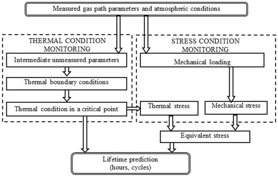
Scheme of the approach used for engine lifetime prediction.

Following the above approach, this article focuses on estimating static thermal boundary conditions, which are necessary to calculate the engine lifetime. Since these conditions are not measured, they are presented by models that employ measured engine parameters as the input data. The article proposes a new method for developing such models using thermodynamic relations between gas path variables. In these relations, some necessary intermediate unmeasured parameters are determined by polynomial functions of the measured quantities. The article emphasizes on the accuracy of the developed models regardless of engine-to-engine differences and an actual healthy or faulty engine condition. The model accuracy is verified on the engine steady-state data simulated by a nonlinear physics-based gas turbine model, also known as thermodynamic model. To take into account different engine health conditions, the data are simulated for both nominal and shifted performance maps of different engine components (compressor, combustion chamber, turbines, etc.). Such simulation of the component degradation is widely used in gas turbine monitoring and diagnostics.^18,19 To confirm a high accuracy of the proposed physics-based method, it is compared with the reference method previously developed in Maravilla et al.²⁰ on the basis of the similarity theory. To finally validate the applicability of the method, the influence of the inaccuracy of the thermal boundary conditions on the errors of engine lifetime prediction is evaluated. To realize and prove the approach briefly described above, a turbine blade is chosen as a test case.

Test case

A turbine blade with three cooling channels (see Figure 2) has been chosen as the critical engine element for which the thermal boundary condition models will be developed. This blade is mounted in the first stage of the high-pressure turbine (HPT) of a two-spool free turbine engine. The eight gas path parameters measured in this engine are as follows:

G_f: fuel consumption;

$T_{C}^{*}$ : compressor discharge temperature;

$p_{C}^{*}$ : compressor discharge pressure;

$T_{HPT}^{*}$ : HPT discharge temperature, also known as exhaust gas temperature (EGT);

$p_{HPT}^{*}$ : HPT discharge pressure;

$T_{LPT}^{*}$ : low-pressure turbine discharge temperature;

$n_{HP}$ : HPT rotation speed;

n_LP: low-pressure turbine rotation speed.

Figure 2.

Critical points in the turbine blade mid-span section.

Based on the experience accumulated in the Zhukovsky National Aerospace University “KhAI” in the analysis of destruction of gas turbine hot elements, the blade mid-span section has been chosen as a critical place. The two-dimensional (2D) analysis of this section was then conducted using the specialized FEA package developed in the university. A mesh has been first generated on the section, and all nodes (points) of the mesh were numbered. A finite model of the blade was then built, the boundary conditions were set, and the distribution of the blade temperature and stress was finally obtained. After the simulation, the points with the minimal safety factor have been chosen. These critical points are the points with numbers 101, 102, 103, and 69. As shown in Figure 2, the first three points are located at the leading edge and the last point is situated at the trailing edge. To make it easier to analyze these critical points, they are divided into two groups: the first group named ga consists of points 101–103 while the second group gb includes critical point 69. The boundary condition models will be created for both groups.

A thermodynamic model is available for the engine under analysis. Such nonlinear physics-based models are widely used in the area of gas turbine diagnostics and are described in detail, for example, in Yepifanov et al.²¹ In this study, the thermodynamic model is not used directly in the boundary condition models developed; it is only a source of data for determining and validating these models.

The rest of the article presents formulation and results related to the test case engine and its test case hot element, turbine first-stage blade. This material is structured as follows. Section “Turbine blade thermal SC” briefly describes the algorithms to compute thermal SCs (temperature and stress in the critical points). This section focuses on the input variables to these algorithms, namely, thermal boundary conditions. Section “Model development methodology” presents a detailed description of the methodology to develop the boundary condition models. Development and verification of these models are given in section “Development and verification of boundary condition models” while section “Models’ accuracy analysis” analyzes their accuracy. Section “Discussion” generalizes the accuracy analysis and shows perspectives of further accuracy enhancement.

Turbine blade thermal SC

In our previous article,²⁰ the models first proposed in Oleynik¹⁷ for calculating the blade temperature and thermal stress were applied to the same test case blade critical points that were described in the previous section. It was concluded after the comparison that the best model of the blade temperature at the critical points is

t_{c r} = T_{S 1}^{*} + Θ (k_{α}) \cdot (T_{S 2}^{*} - T_{S 1}^{*})

(1)

where $t_{cr}$ is the blade temperature at a critical point, $T_{S 1}^{*}$ the cooling temperature, $T_{S 2}^{*}$ the heating temperature, $Θ$ the dimensionless parameter, and $k_{α} = α_{i} / α_{ref}$ the relation of the heat transfer coefficients at current and reference engine operating modes, respectively.

It was also found that the best model to estimate the thermal stress is given by

σ_{t} = \bar{S} (k_{α}) \cdot n^{2}

(2)

where $σ_{t}$ is the thermal stress at a critical point, n the rotational speed, and $\bar{S}$ is the dimensionless parameter.

The dimensionless parameters $\bar{S}$ and $Θ$ are calculated using polynomial functions as dependence of the coefficient $k_{α}$ that is a generalized parameter that depends on two particular quantities, coefficient k_αS₁ for a cooling surface and coefficient k_αS₂ for a heating surface.

The four parameters $T_{S 1}^{*}$ , $T_{S 2}^{*}$ , k_αS₁, and k_αS₂ that are the input data in equations (1) and (2) are called thermal boundary conditions. Since they are usually unmeasured, numerous alternative models to calculate these conditions are developed and compared in this study to choose the best model for each boundary condition. In this way, the accuracy of equations (1) and (2) is improved by choosing the best models for estimating the thermal boundary conditions, which are the input data of these equations. In its turn, the lifetime prediction that uses temperature (equation (1)) and stress (equation (2)) as the input data will be enhanced as well. The next section describes the methodology used for developing different boundary condition models and chooses the best model for each condition.

Model development methodology

Determination of the boundary condition models

Given that the models of the boundary conditions are intended for on-line monitoring, they must meet the following main requirements:

All the models must use the gas path measuring parameters as the input data.

The models should have a simple structure, making it possible to use them in real time.

The measurement errors of the gas path parameters, which are the input data of the models, must be taken into account.

The models should have a high robustness to changes in engine health conditions.

To meet these requirements, it is proposed to develop models based on the use of basic physical relations, such as mass and energy conservation equations, thermodynamic relations, and kinematic relations, which describe the motion of the working fluid.

Let us introduce the following designations:

Z: vector of unmeasured parameters to estimate (thermal boundary conditions);

Y: vector of gas path measured parameters;

W: vector of intermediate unmeasured parameters that characterize the thermodynamic properties of the working fluid, such as efficiencies and pressure loss factors;

$T_{H}^{*}, p_{H}^{*}$ : ambient conditions (temperature and pressure).

Taking into account the requirements previously considered, the general dependence for a boundary condition z can be given by a general function

z = f (Y, W, T_{H}^{*}, p_{H}^{*})

(3)

However, expression (3) cannot be computed in practice as long as the parameters of vector W are unknown. To determine each necessary parameter w, it is proposed to describe it as a function A (internal model) that has as an argument one of the measured parameters x defining the engine operation mode. Thus, the function looks as w = A(x), where x is measured. All the function parameters are corrected to standard atmosphere (temperature of 288.15 K and pressure of 101.3 kPa) to take into the account the influence of the atmospheric conditions.²² With regard to this assumption, expression (3) is rewritten and further used as

z_{c o r} = f (Y_{c o r}, A (x_{c o r}))

(4)

To better illustrate the above-described algorithm of the development of the boundary condition models, Figure 3 presents the block diagram of this development. Using the mentioned algorithm, the models for the four necessary boundary conditions $T_{S 1}^{*}$ , $T_{S 2}^{*}$ , k_αS₁, and k_αS₂ are developed.

Figure 3.

Algorithm for developing the boundary condition models.

Model verification

As stated in the model requirements, gas path measured parameters are the input data for the boundary condition models. To choose which measured parameter should be used as an argument in each internal model, a total mean square error (MSE) is computed to be used as a criterion. The total MSE $σ_{TT}$ characterizes the robustness and accuracy of the boundary condition model and consists of two components: truncation error $σ_{TR}$ and instrumental error $σ_{INS}$ . In this way

σ_{T T} = σ_{T R} + σ_{I N S}

(5)

Truncation error

The mean square truncation error for one health condition is calculated as

σ_{T R j} = \sqrt{\frac{\sum_{j = 1}^{N_{j}} {(z_{j i m} - z_{j i})}^{2}}{N_{j}}}

(6)

and the average error percentage for all conditions is given by

σ_{T R m} = \frac{1}{n} \sum_{j = 1}^{n} σ_{T R j} \cdot 100 %

(7)

where value z_{j m} is calculated by the boundary condition model, z_{i j} is a true value generated by the thermodynamic model, N_j stands for the sample size (number of the engine operating points) for the engine health condition number j, and n denotes the number of engine health conditions.

Instrumental error

The MSE of the instrumental error is calculated for one health condition according to an expression

σ_{INS} = \sqrt{{\sum_{q = 1}^{Q} (\frac{\partial z}{\partial y_{q}})}_{i} \cdot σ_{y q}^{2} + {\sum_{k = 1}^{K} (\frac{\partial z}{\partial x_{k}})}_{i} \cdot σ_{x k}^{2} + {(\frac{\partial z}{\partial T_{H}^{*}})}_{i} \cdot σ_{T_{H}^{*}}^{2} + {(\frac{\partial z}{\partial p_{H}^{*}})}_{i} \cdot σ_{p_{H}^{*}}^{2}}

(8)

and on average is given by

σ_{I N S m} = \frac{1}{N} \sum_{j = 1}^{n} σ_{I N S j} \cdot 100 %

(9)

where N is the number of the engine operation modes for a healthy engine.

Robustness analysis

All true data corresponding to a healthy engine and 10 deteriorated (faulty) engine conditions were simulated using the thermodynamic model.²¹ These conditions are determined by the fault parameters that shift by 3% the performances of engine components as shown in table 1. The instrumental error was calculated for each of these deteriorated engine conditions using expressions (8) and (9).

Table 1.

Engine component deterioration conditions simulated by the thermodynamic model.

Designation	Fault parameter	Deteriorated condition
C0	−	Healthy engine
C1	δη_C	Compressor efficiency decrease
C2	δG_C	Compressor air flow decrease
C3	δη_CC	Combustion chamber efficiency decrease
C4	δσ_CC	Decrease in the combustion chamber total pressure
C5	δη_HPT	HPT efficiency decrease
C6	δF_{NB HPT}	HPT nozzle box area increment
C7	δσ_HPT-LPT	Decrease in the total pressure between HPT and LPT
C8	δη_LPT	LPT efficiency decrease
C9	δF_{NB LPT}	LPT nozzle box area increment
C10	δG_ST	Increment of the air bleed for gas pumping station needs

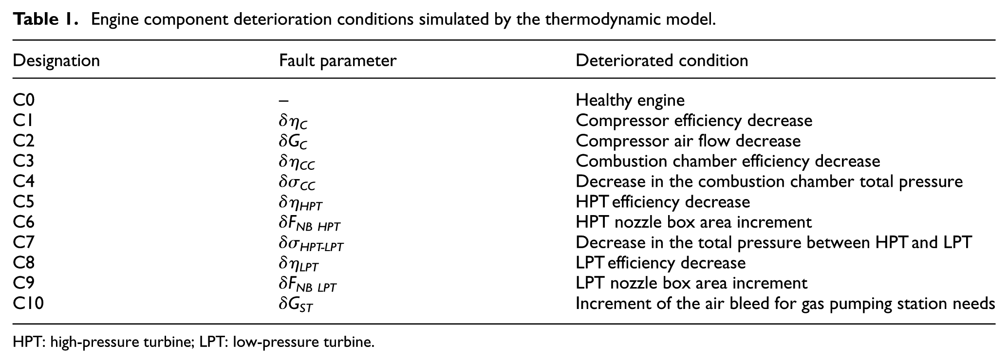
HPT: high-pressure turbine; LPT: low-pressure turbine.

Development and verification of boundary condition models

Models’ development

As described in section “Turbine blade thermal SC,” to estimate the turbine blade thermal SC according to equations (1) and (2), it is necessary to specify the initial data, thermal boundary conditions $T_{S 1}^{*}$ , $T_{S 2}^{*}$ , k_αS₁, and k_αS₂.

For this study, the following particular gas path parameters have been chosen for the boundary temperatures:

The cooling temperature: $T_{S 1}^{*} = T_{C}^{*}$ ;

The heating temperature: $T_{S 2}^{*} = T_{W}^{*}$ .

where $T_{C}^{*}$ is the compressor discharge temperature, and $T_{W}^{*}$ presents the temperature of gases in relative motion in front of the first turbine stage.

Alternative models for all the four boundary conditions have been developed. Although the compressor discharge temperature is a measured parameter in the test case engine, the models of this parameter were developed as well. This allows estimating a positive effect from the inclusion of parameter $T_{C}^{*}$ in a measurement system on lifetime monitoring. Since many alternative models were developed, only two of them are described in depth and given below as examples.

Example 1: model of the compressor discharge temperature

For developing the model, we use the thermodynamic relation that describes the work of compression L_c

L_{C} = C_{p} \cdot (T_{C}^{*} - T_{H}^{*}) = C_{p} \cdot T_{H}^{*} \cdot [{(\frac{p_{C}^{*}}{p_{H}^{*}})}^{\frac{k - 1}{k}} - 1] \cdot \frac{1}{η_{C}^{*}}

(10)

where k is the isentropic factor, C_p is the specific heat at constant pressure, and $η_{C}^{*}$ is the efficiency of compression.

As in expression (10), the parameters k and $η_{C}^{*}$ are unmeasured; instead of them, internal models $A_{1} = (k - 1) / (k)$ and $A_{2} = 1 / η_{C}^{*}$ are introduced. These models are calculated as a polynomial function of an engine power set parameter that is measured. If the rotation speed n is such a parameter, the functions are written by A₁ = f(n_cor); A₂ = f(n_cor).

Solving equation (10) for $T_{C}^{*}$ and making correction to the standard ambient conditions, we arrive at the following expression

T_{C_{cor}}^{*} = T_{0} {1 + A_{2} [{(\frac{p_{C_{cor}}^{*}}{p_{0}})}^{A_{1}} - 1]}

(11)

After an inverse correction, we have the necessary model of the compressor discharge temperature $T_{C}^{*}$ . Let us consider the second example, namely the model of the heat transfer coefficient at the leading edge of the blade.

Example 2: model of the heat transfer coefficient

According to Kopelev,²³ a basic expression for the model is

\frac{α \cdot L}{λ} = A \cdot R e^{d} \cdot K_{rot}

(12)

where $Re = (ρ \cdot W \cdot L) / (μ)$ ; $K_{rot} = 1 + Z \cdot ((u \cdot h) / (W \cdot D))^{q}$ ; K_rot is the coefficient that takes into account the influence of rotation; $α$ , $λ$ , and $μ$ are the heat transfer, heat conductivity, and dynamic viscosity coefficients, respectively; A, d, Z, and q are the constants; L is the hydraulic diameter; D is the blade section diameter; u is the circumferential speed; h is the blade length; $ρ$ is the viscosity; and W is the relative velocity.

According to Kopelev,²³ $μ = T^{0.64}$ and $λ = T^{0.76}$ . Taking into account the above definitions, expression (12) is rewritten for the heat transfer coefficient resulting in

α_{i} = A \cdot {(\frac{p_{1} \cdot W_{1} \cdot L}{R_{g} \cdot T_{1} \cdot μ_{1}})}^{d} \cdot [1 + Z {(\frac{π \cdot n_{HP} \cdot h}{60 \cdot W_{1}})}^{q}] \cdot \frac{λ_{1}}{L}

(13)

To compute this coefficient, the following values were used: A = 0.74, Z = 0.20, L = 3.4 × 10⁻² m, h = 4.57 × 10⁻² m, D = 0.6075 m, d = 0.5, and q = 0.17. To determine the other necessary variables p₁, w₁, and T₁ at the entrance of the blade, the corresponding internal models were developed using polynomial functions.

Structure of the alternative models developed

In total, for all the boundary conditions, the alternative models for the following unmeasured boundary conditions $T_{C}^{*}$ and $T_{W}^{*}$ as well as intermediate parameters p₁, w₁, and T₁ were developed according to the method presented in Figure 3. Several models were developed based on different source expressions. Figure 4 shows a general scheme for developing alternative models. According to this scheme, a total of 31 models were developed. Their names and arguments are shown in Figure 5. Appendix 3 contains a detailed list of these models.

Figure 4.

Scheme of the development of the alternative models.

Figure 5.

Structure of the alternative models developed.

Models’ verification

As a result of the internal model verification, the measured parameter used as argument and the degree of the polynomial were chosen for each internal model A(x). Let us consider as an example the model MTG1 that is used to monitor the gas temperature $T_{g}^{*}$ at the inlet of the turbine. This model has the following structure

T_{g cor}^{*} = A_{TG 1} \cdot (T_{C cor}^{*} - T_{0}) + T_{HPT cor}^{*}

(14)

where $A_{TG 1} = (C_{p a} / C_{p g}) \cdot (ν / η_{m})$ ; $ν = G_{a} / G_{g}$ ; C_{p a} and C_{p g} are the air and gas specific heat at constant pressure, respectively; G_a and G_p are the air and gas consumption, respectively; $T_{HPT}^{*}$ is the gas temperature after the HPT.

The model MTG1 includes an internal model that describes A_TG₁ as a function of the mechanical efficiency $η_{m}$ , specific heat coefficients C_{p a}, and C_{p g}, and the relative consumption $ν$ . This internal model is defined as a polynomial function of a measuring gas path parameter A_TG₁ = f(x). The engine analyzed has eight gas path measuring parameters, and it is necessary to determine which one of them can be used as a function argument and what degree of polynomial is the best.

All the necessary data to obtain the value of the coefficients in the polynomial are obtained with the help of the thermodynamic model.²¹ These data were generated for a healthy engine condition at 245 operating modes uniformly distributed in space of the operating conditions. The generated data were then divided into two sets: reference set of 123 modes and validation set of 122 modes. Using the reference set, the polynomial coefficients were estimated by the least squares method. Many alternative polynomial functions were determined: polynomial degree was changed from 1 to 4 and different gas path parameters were used as a function argument.

After determining the coefficients for all the polynomials that describe the internal model A_TG₁, the value of $T_{g}^{*}$ was calculated as follows

T_{g}^{*} = [A_{TG 1} (x) \cdot (T_{C cor}^{*} - T_{0}) + T_{HPT cor}^{*}] \cdot \frac{T_{H}^{*}}{T_{0}}

(15)

The total error calculated using expression (5) is the main criteria to judge the accuracy of the monitoring models. The necessary truncation and instrumental errors were calculated on the validation set data using equations (6)–(9).

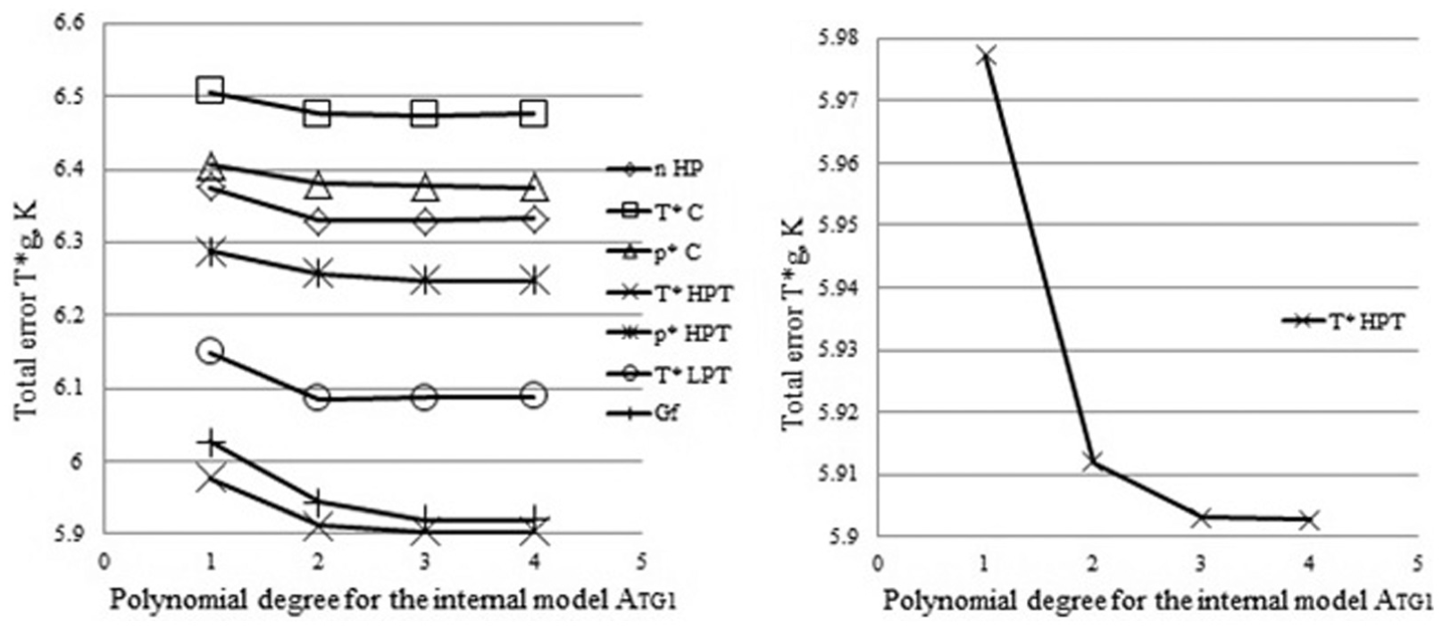
To test the model robustness, the truncation error was computed using expressions (6) and (7). The calculation was performed for one healthy and 10 faulty engine conditions (see Table 1) with the help of the thermodynamic model. The total error in the prediction of $T_{g}^{*}$ using model MTG1 is illustrated in Figure 6.

Figure 6.

Total $T_{g}^{*}$ error against the polynomial degree and different polynomial function arguments for model MTG1: (a) seven different arguments and (b) the best argument.

From Figure 6(a), it is clear that the best prediction of $T_{g}^{*}$ is obtained when the internal models are described by the measuring temperature $T_{HPT}^{*}$ . A more detailed analysis (Figure 6(b)) shows that it is sufficient to use a third-degree polynomial, since further increment in the degree of polynomial has no effect on the total error. According to the results, model MTG1 has the following structure

T_{g}^{*} = [A_{TG 1} (x) \cdot (T_{C cor}^{*} - T_{0}) + T_{HPT cor}^{*}] \cdot \frac{T_{H}^{*}}{T_{0}}

(16)

where $A_{TG 1} (x) = - 6.79 \cdot 10^{- 10} \cdot T_{HPT cor}^{* 3} + 2.19 \cdot 10^{- 6} \cdot T_{HPT cor}^{* 2} - 2.47 \cdot 10^{- 3} \cdot T_{HPT cor}^{*} + 1.87$ .

In the same way as in the above example of model MTG1, the best measured parameters used as arguments in the i-internal models and the best polynomial degree were selected for all the developed models. After the models’ verification, the finally selected models for all boundary conditions are presented in Figure 7.

Figure 7.

Selected models to monitor the thermal boundary conditions of the HPT first-stage blade.

Models’ accuracy analysis

Estimation of thermal boundary conditions

This section compares the accuracies of two different approaches for model development: physics-based models proposed in this article and the models previously developed with the help of the theory of similarity (reference models, see Oleynik¹⁷).

The models are compared for each of the four thermal boundary conditions, namely:

Cooling temperature: $T_{S 1}^{*} = T_{C}^{*}$ ;

Heating temperature: $T_{S 2}^{*} = T_{W}^{*}$ ;

Relation $k_{α g} = α_{i g} / α_{ref g}$ for the heat exchange with hot gases;

Relation $k_{α a} = α_{i a} / α_{ref a}$ for the heat exchange with cooling air.

The truncation errors of the estimation of these boundary conditions are presented in Figure 8 for four boundary variables and 11 health conditions. Analysis of these errors shows that on average the proposed models (blue color) are more accurate than the previous models.

Figure 8.

Truncation errors in the estimation of the thermal boundary conditions for different engine health conditions: (a) $T_{W}^{*}$ , (b) $T_{C}^{*}$ , (c) $k_{α g}$ , and (d) $k_{α a}$ ; blue color: physics-based models; red color: models developed on the theory of similarity.

The above accuracy analysis has been performed using the thermodynamic model as a reference and theoretical distribution of simulated errors. Nevertheless, this type of models has its intrinsic errors, and real measurement errors differ from the simulated ones. Therefore, it is important to try to verify the methodology of estimating unmeasured gas turbine parameters using empirical information. Fortunately, such information is available for the engine under analysis.

Accuracy analysis on real data

For the analyzed engine, the cooling temperature $T_{S 1}^{*} = T_{C}^{*}$ is a measured parameter (see section “Test case”), and it is not practically interesting to verify its accuracy. On the other hand, a heat transfer coefficient is too difficult to measure. For these reasons, the parameter most interesting for accuracy analysis is the heating temperature $T_{S 2}^{*} = T_{W}^{*}$ . However, this parameter is unmeasured because of too high temperatures in front of the first turbine stage. Since it is difficult to directly verify the accuracy of the heating temperature on real data, the following indirect verification is proposed.

The empirical information available for the engine presents steady-state measurements averaged and hourly recorded at field conditions, also known as snapshots. Since parameter $T_{W}^{*}$ is not among the recordings, let us choose the nearest measurement station (see section “Test case”), HPT discharge, and use EGT $T_{HPT}^{*}$ to verify a general possibility to estimate unmeasured hot part temperatures using measured gas path parameters and ambient conditions. Let us imagine that the EGT is not measured and create an EGT model as a function of the measured quantities. Such a data-driven model was created using a reference set of 1200 consecutive snapshots that include periods of compressor fouling (the most frequent mechanism of degradation of stationary gas turbines) and one compressor washing. For this EGT model, the average accuracy was determined on the extended set of 2000 snapshots (including the reference set) by comparing the EGT estimations and real measurements. This accuracy works out 0.085%. Considering that this number is obtained in the presence of engine degradation that increases the EGT by 1.8%, we can state that the EGT estimation through the other measured quantities is pretty accurate. Since there is no reason to suppose that the $T_{W}^{*}$ estimation should be less accurate, we can hope that in practice the accuracy of the estimated temperature $T_{W}^{*}$ will not be worse.

Thus, the above two sections dealt with accuracy of thermal boundary conditions themselves. The following two sections analyze how the boundary condition accuracy influences the accuracy of thermal stress and lifetime estimation.

Thermal stress estimation and lifetime prediction when the compressor temperature is not measured

The turbine blades’ thermal SC was assessed using expressions (1) and (2). The prediction of the lifetime of turbine blades is a very complex process in which a significant number of factors influence. Our study analyzes the impact that a new method to develop models has on the accuracy of the lifetime prediction. This makes possible to use a conservative prediction of the lifetime, which will be sufficient to assess the adequacy of the developed physics-based models.

One of the simple and easy practical ways to determine the lifetime is the Larson–Miller relation

t_{r} = 10^{\frac{PLM}{t_{cr}} - C}

(17)

where PLM is the Larson–Miller parameter; C is the coefficient that for our test case has the value of 20.

Two cases are considered:

When the thermal boundary conditions are calculated with the physics-based models;

When the thermal boundary conditions are calculated with the models developed using the theory of similarity.

The analysis of the results presented in Figure 9 shows that the use of physics-based models leads to a better estimation of TC (Figure 9(a)) and better prediction of lifetime t_r (Figure 9(e)). On the other hand, the prediction on SC is less affected (Figure 9(c)).

Figure 9.

Total error in the prediction of TC, SC, and t_r. Blue color: physics-based models; red color: models based on the theory of similarity. (a, c, e) $T_{C}^{*}$ is a unmeasured parameter; (b, d, f) $T_{C}^{*}$ is a measured parameter.

It is clear that the choice of the models to estimate the thermal boundary conditions affects the results in the prediction of lifetime t_r for both groups of critical points ga and gb. For example, for the group of critical groups ga, the results show that the use of physics-based models to calculate the thermal boundary conditions reduces the errors of the temperature at the critical point t_r from 1.03% to 0.59%. The lifetime errors reduce from 102.8% to 40.94% accordingly. We can observe a similar error change for the group of critical points gb. It can be concluded that the accuracy of the lifetime prediction is enhanced due to a more accurate estimation of the material temperature t_cr by physics-based models.

The previous results were obtained when the temperature after compressor $T_{C}^{*}$ is an unmeasured parameter.

Thermal stress estimation and lifetime prediction when the compressor temperature is measured

A temperature after compressor $T_{C}^{*}$ is not included in a standard measurement system. Therefore, it is of particular interest to know how its installation influences the accuracy of thermal stress and lifetime estimates. To this end, all the previous calculations were later repeated considering that the temperature after compressor $T_{S 1}^{*} = T_{C}^{*}$ is a measured parameter. The values of this temperature were obtained using the thermodynamic model.²¹

The results in the calculations of the TC, SC, and t_r are presented in Figure 9. The analysis of this figure shows that for the case of the physics-based models, the level of errors for the critical points ga decreases from 0.58% to 0.44%. This leads to a better prediction of lifetime t_r (errors decrease from 45.95% to 27.96%). The accuracy in the prediction of t_r for the critical points gb is also enhanced.

Thus, we can conclude that the measurement of the cooling temperature $T_{S 1}^{*} = T_{C}^{*}$ has a significant effect on the accuracy of the prediction of lifetime t_r. For example, if $T_{C}^{*}$ is measured, the errors in the prediction of t_r for the group of critical points ga reduce from 102.8% to 45.95% for the case of the physics-based models.

Discussion

The analysis performed in the previous section proves high accuracy of the developed models for the thermal boundary conditions. However, we need to keep in mind that the reference data employed to determine the models’ accuracy were also simulated. Let us discuss the following two issues:

Proper interpretation of the accuracy analysis performed in section “Models’ accuracy analysis” on simulated data;

Perspectives of further accuracy enhancement using real reference data.

The first issue is related to the boundary condition errors and stress and lifetime inaccuracy. To estimate the boundary condition errors, the thermodynamic model was employed in the article. Unfortunately, this model has its intrinsic errors, and, consequently, the boundary condition errors will possibly grow in practice.

When the stress and lifetime inaccuracy were determined in sections “Thermal stress estimation and lifetime prediction when the compressor temperature is not measured” and “Thermal stress estimation and lifetime prediction when the compressor temperature is measured,” the errors of only the thermal boundary conditions were taken into consideration, and the other errors determined in the thesis¹⁷ were not. This is natural because the boundary conditions are a principal object investigated in this article, and the article results show the possibility of real application of the proposed methodology. However, the above reasoning implies possible growth of the errors of lifetime monitoring under real conditions.

Within the second issue, the possibility of the enhancement of lifetime prediction is discussed. The point is that the thermodynamic model is used in this study only for data generation to determine and validate the boundary condition models. Thus, the thermodynamic model is not a part of the proposed methodology and can be replaced by real data. Although a standard measurement system is not sufficient for this purpose, additional instrumentation can be installed under engine test bed conditions. In this way, we can completely replace the thermodynamic model by real data and exclude all simulation errors.

There is another way to easily enhance the boundary condition and lifetime accuracy. In the analysis described in section “Models’ accuracy analysis,” the simulated measurement errors correspond to a single parameter recording time station. By uniting some consecutive stations for estimating average parameters, it is possible to further enhance the boundary condition and lifetime estimates.

Conclusion

The article proposes the method to develop simplified physics-based models for estimating the unmeasured thermal boundary conditions for hot elements of gas turbines. A turbine blade has been chosen as a test case for the proposed method. The blade is mounted in the first stage of the HPT of a two-spool turbo shaft engine. In the simplified models, the necessary intermediate unmeasured parameters were defined via internal polynomial functions (internal models). To determine polynomial coefficients by the least squares method, a great volume reference set with measured and unmeasured gas path parameters has been generated by the nonlinear thermodynamic model. To choose the best internal model of each intermediate parameter, a total of 31 alternative candidate models were developed. The best measured parameter used as an argument of the polynomial functions and the degree of polynomials was chosen for each candidate model. The candidates tailored in this manner on the reference set data were then compared using a validation set generated by the thermodynamic model for healthy and many faulty health conditions. The truncation and instrumental errors as well as the model robustness to engine faults were the criteria to choose the best candidate for each internal model. Finally, the internal models optimized in this manner were used in the simplified models of the boundary conditions.

Two methodologies for the development of the boundary condition models were compared: physics-based methodology (proposed in this article) and similarity-based methodology (reference). The results show that the physics-based methodology is less sensitive to engine faults and always provides a better estimation. It was found that the use of this methodology improves the estimates of the thermal boundary conditions, which lead to considerable improvement in the estimation of the temperature at the critical point and in the prediction of the lifetime. For example, the results show that the use of physics-based methodology reduces the errors of this temperature from 1.03% to 0.59%, which leads to reduction in the lifetime prediction errors from 102.8% to 40.94%. These results correspond to the case when the compressor discharge temperature is not measured.

It was proven that the measurement of the compressor discharge temperature $T_{C}^{*}$ in addition to standard gas path measurement system dramatically improves the effectiveness in the prediction of the lifetime. For example, the errors in the thermal boundary conditions can be lowered by 60%.

In this way, all the results of the accuracy analysis prove that after several stages of optimization, the developed thermal boundary condition models have acceptable accuracy. The discussion section shows the ways of further improvement of these models using real data.

Footnotes

Appendix 1

Appendix 2

Appendix 3

Academic Editor: Yonghui An

Declaration of conflicting interests

The author(s) declared no potential conflicts of interest with respect to the research, authorship, and/or publication of this article.

Funding

The author(s) disclosed receipt of the following financial support for the research, authorship, and/or publication of this article: This study was performed with the support of the National Polytechnic Institute of Mexico.

References

Jin

Lodwen

Pistor

. Remaining life assessment of power turbine disks. ASME paper GT2008-51010, 2008.

Alexander

. Gas turbine plant thermal performance degradation assessment. ASME paper GT2008-50032, 2008.

Phillip

David

. Remaining life assessment technology applied to steam turbines and hot gas expanders. ASME paper GT2011-45324, 2011.

Zbigniew

Edoskopic examinations of marine diesel engine’s turbocharging systems. J Pol CIMAC 2008; 4: 111–119.

Hunik

Rooth

. TINTELL: an innovative method for blade life management. ASME paper GT2002-30055, 2002.

Wan

John

Paul

. Combustion turbine F-class life management of 1st stage turbine blades. ASME paper GT2002-30301, 2002.

Letcher

Herman

Onome

. An energy based critical fatigue life prediction method. ASME paper GT2011-45443, 2011.

Wertz

Herman

Onome

. An energy based axial isothermal-mechanical fatigue lifing procedure. ASME paper GT2011-45261, 2011.

Giuseppe

Carlevaro

. Gas turbine maintenance policy: a statistical methodology to prove interdependency between number of starts and running hours. ASME paper GT2002-30281, 2002.

10.

Parthasarathy

Menon

Richardson

. Neural network models for usage based remaining life computation. ASME paper GT2006-91099, 2006.

11.

Yoon

Kim

Lee

. Simulation of performance deterioration of a microturbine and application of neural network to its performance diagnosis. ASME paper GT2008-51494, 2008.

12.

Fast

Assadi

. Condition based maintenance of gas turbines using simulation data and artificial neural networks: a demonstration of feasibility. ASME paper GT2008-50768, 2008.

13.

Palme

Breuhaus

Assadi

. Early warning of gas turbine failure by nonlinear feature extraction using an auto-associative neural network approach. ASME paper GT2011-45991, 2011.

14.

Blumenthal

Hutchinson

Zori

. Investigation of transient CFD methods applied to a transonic compressor stage. ASME paper GT2011-46635, 2011.

15.

Weiss

Subramanian

Hall

. Simulation of unsteady turbomachinery flows using an implicitly coupled nonlinear harmonic balance method. ASME paper GT2011-46367, 2011.

16.

Jeromin

Eichler

Noll

. Full 3D conjugate heat transfer simulation and heat transfer coefficient prediction for the effusion-cooled warm of a gas turbine combustor. ASME paper GT2008-50422, 2008.

17.

Oleynik

. Concepts and development of methods for lifetime monitoring based on the identification of the dynamics of the thermal-stress conditions of aviation gas turbine engine critical components. Thesis for scientific degree of the Doctor of Science (Engineering) on the speciality 05.07.05, Aircraft engines and power plants, Zhukovsky National Aerospace University, “KhAI”, Kharkiv, 2006.

18.

Romessis

Kamboukos

Mathioudakis

. The use of probabilistic reasoning to improve least squares based gas path diagnostics. ASME paper GT2006-90619, 2006.

19.

Borguet

Leonard

. A generalized likelihood radio test for adaptive gas turbine health monitoring. ASME paper GT2008-50117, 2008.

20.

Maravilla

Yepifanov

Loboda

. Improved turbine blade lifetime prediction. ASME paper GT2015-43046, 2015.

21.