
Abstract
In transportation planning works, critical links identification is helpful to evaluate the vulnerable parts of the designed network schemes. A new capacity-based network robustness index is presented for identifying critical links and evaluating the transportation system performance. It uses the change of the total network capacity as an evaluation measure. The advanced practical network capacity model is employed to estimate the throughput of transportation system. A sensitivity analysis based algorithm is also developed to solve the practical capacity model efficiently. The capacity-based network robustness index identifies the links which play critical roles in the transportation capacity of the whole network. The capacity-based network robustness index is an effective supplementary to the existing network evaluation indices. The experiments demonstrate the differences between the capacity-based network robustness index and the efficiency-based network robustness index. The capacity-based network robustness index can be used as a practical measure in the situations where the network robustness index is not significant.
Keywords
Introduction
In the studies of transportation systems, the disruption of transportation network has been drawing much attention of researchers because of natural disasters, terrorist attacks, and traffic accidents during the past two decades. The transportation system is vital to people’s health, safety, comfort, and economic activities as lifelines nowadays. 1 As a result, a large number of literatures sprang up, which focus on network disruption when network components are degraded or blocked. As experience shows, the blockages or failures of the network links that are heavily traveled or those containing bridges could have serious impacts on the whole transportation network. But there are many potential ordinary road segments whose losses of function also create system-wide influence. Hence, various measures for network performance evaluation have been developed in previous research.
Network vulnerability analysis finds the vulnerable components in a transportation network. It is applied to identify the critical links or nodes in the system to maintain its robustness. The approaches generally evaluate the impact on the system-wide performance as the degradation or removal of a single link. The evaluation indicators can be total travel time (TTT),2,3 connectivity,4,5 and accessibility.1,6
In practical transportation planning, the localized level of service is an often-used indicator for measuring link-level vulnerability. It utilizes the volume-to-capacity (V/C) ratio to reflect the network congestion. Although the V/C ratio has been used to address some complex decision-making in transportation management, it may not enable the traffic engineers to identify the most critical components in system-wide. 7 Similar link-based indicators can be found in Knoop et al. 8
The network robustness index (NRI) is a direct measure to reflect how vulnerable a single link is if it was completely removed. The NRI takes into account the spatial relationships and rerouting possibilities associated with the network’s topology, the origin and destination (OD) demand, and the capacity of individual highway segments. 7 The NRI employs the TTT in system-wide as a measurement, so as to reflect the change in transportation efficiency of the network. Using this indicator, the most critical links in the transportation network can be ranked by their effect to the system-wide efficiency. Nevertheless, this indicator based on travel time is not significant to reflect the throughput capacity of the transportation system. In the following section, we present a counter-example to show the insufficiency of the travel-time-based indicator.
Network reliability also reflects the system-wide performance when the supply or the capacity of system components is uncertain. The reliability indices are generally expressed as a multiplier of the probability that a specific event and the consequence of that event may occur. These include the following: network connectivity reliability, which is the probability that network nodes are connected; travel time reliability, which is the probability that a trip between a given OD pair can be made successfully within a given time interval and a specified level of service; and capacity reliability, which is the probability that the network capacity can accommodate a certain level of traffic demand.9–11 The reliability provides a probabilistic assessment of transportation networks under uncertainty. However, reliability is a user-oriented quality of the transportation system, while robustness, however, is a characteristic of the system itself. Thus, the robustness is more effective for network vulnerability analysis.
Furthermore, the concept of road network capacity is conducted to reflect how many travel demand can be allocated by a given road network. Wong and Yang 12 first proposed the reserve capacity model. Since the network capacity plays an important role in transportation infrastructure planning and evaluating, it is still now a hot topic in transportation network modeling and widely used. On the basis of the reserve capacity, Wang et al. 13 conducted a model incorporated with the stochastic user equilibrium, in order to determine the optimal investment strategy to improve the total road network capacity. Xu et al. 14 employed the reserve capacity with multi-mode to discuss the redundancy of the urban transport network. Although the reserve capacity model is easy to use, its assumption that all OD demands increase in the same rate is rather impractical. Beyond the reserve capacity model, Gao and Song 15 extended the reserve capacity model by considering OD-specific demand multipliers. Also, the concepts of ultimate capacity and practical capacity are proposed to conquer the drawbacks of the reserve capacity model.16,17
Hence, a new evaluation index is proposed in this article, that is, capacity-based network robustness index (CNRI). We defined the CNRI as the change in the total capacity of the network when a single link loses its own capacity. This new measure showed several merits according to the comparative experiments with the NRI. The reminder of this article is organized as follows. Section “Index for transportation network robustness” describes the formulation of the NRI. In section “Overview of network capacity models,” the network capacity model is introduced along with an efficient solution algorithm, following a simple case that illustrates the limitation of the NRI. The concept of CNRI is defined and formulated in section “CNRI.” In section “Numerical results,” the numerical experiments show the special features of the CNRI compared to the NRI. Finally, a short conclusion is summarized in section “Conclusion.”
Index for transportation network robustness
NRI
The original formulation of the NRI is proposed by Scott et al. 7 The NRI evaluates how critical a given link is to the overall transportation network. A link is more critical if its removal results in a relatively high increase in the TTT in system-wide. The NRI provides the transportation planners with objective information beyond anecdotal observations and is straightforward to be calculated using the traffic assignment tools. 18
The NRI is defined as the change in the TTT resulted from the reassignment of the travel demand in the network when a specific link is removed. It was presented as an alternative to both the V/C ratio and the network-wide gamma index for network connectivity. 7
The NRI is produced in two steps. First, the TTT is calculated when all links in the network are present. The TTT is given by the sum of the product of the travel time and traffic flow on each link in the network

where s is the TTT of the transportation network; ta is the travel time through link a at current traffic level, va; and A is the set of all links in the network. In applications, it is more realistic to represent the link travel time as a function of the flow on it, that is, ta = ta(va). 7
In the second step, the TTT is derived for each link a in the network when the individual link a is completely removed. It is obtained by

where sa is the TTT of the rerouted traffic flow after the removal of link a. Thereby, the NRI for link a is calculated as the change of the TTT by removing link a

To demonstrate the traffic flow change in system-wide, the user equilibrium assignment is employed for the evaluation of the NRI. It is also shown that the TTT is not always increased by removing a single link, so the value of NRI can be either positive or negative. The presence of the network robustness provided a novel approach to identify the critical links in a transportation network. The comparative experiments showed that the evaluation of a network using the NRI gives a better planning solution than those obtained using the traditional localized V/C ratio. 7 This approach is able to help with decision-making for emergency preparedness, supply-chain logistics, and network robustness. The NRI was further extended for the situation that the link capacity degrades in different levels. 18
A counter-example of NRI application
When the NRI was proposed, it was stated to have a better performance than the traditional V/C ratio. However, the NRI maybe not always reliable for the transportation network where complex OD relationships exist. A potential problem is illustrated in Figure 1 with two OD pairs. The travel demand from node 1 to node 2 is set to three, and the demand from node 1 to node 3 is one. Suppose that the link performance functions of all links is given by
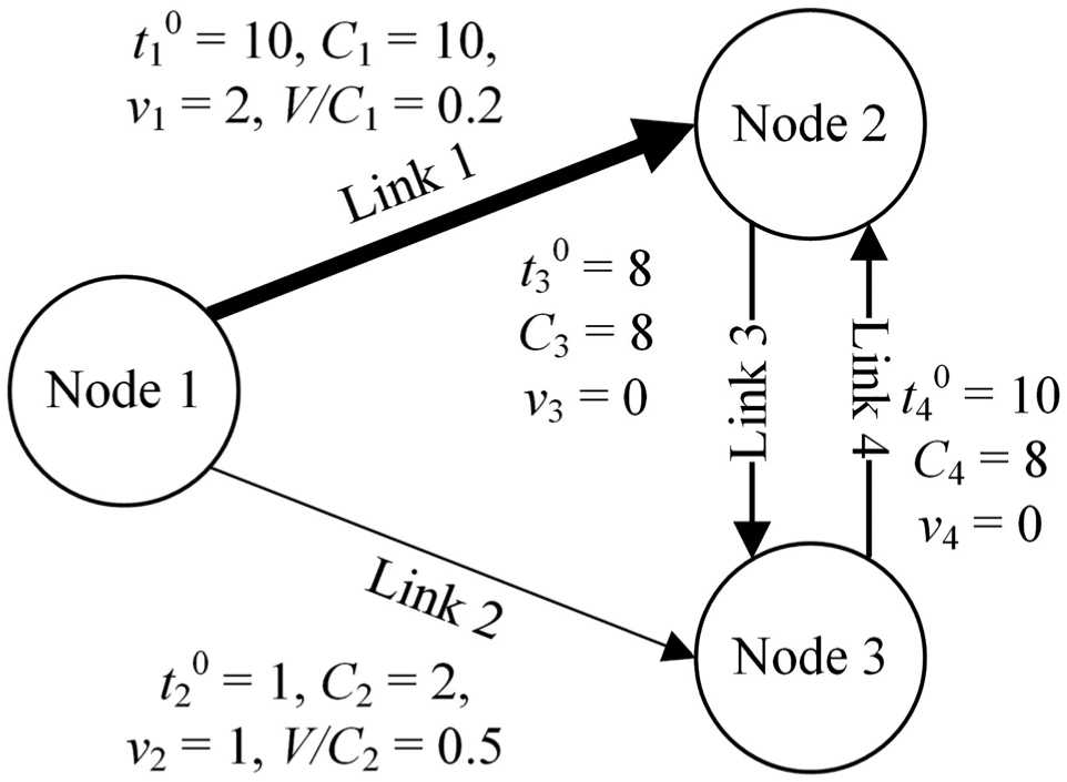
Example of critical links using NRI.
In this case, there is no traffic flow traverses in links 3 and 4. Obviously, the V/C ratios suggest that link 2 is the most critical link. Furthermore, the values of the NRI (NRI1 = 4.276 and NRI2 = 17.023) also indicate that link 2 is more critical. However, link 1 carries the most traffic demand in the transportation system. If link 1 was removed, the traffic from node 1 to node 2 would reroute to links 2 and 4. Thus, the flow in link 2 will exceed its capacity, which causes the failure of link 2 by traffic congestion. However, if link 2 was eliminated, rerouted traffic can be easily accommodated by links 1 and 3. Hence, link 1 is actually more critical to the network than the other links. In the above case, neither V/C ratio nor NRI is effective to represent the importance of links to the transportation network.
In summary, the TTT with the framework of equation (1) reflects the efficiency of the total travels. Although only a small number of drivers increase their travel time significantly (such as the counter-example), the TTT could be increased further. Another drawback of the efficiency-based evaluation is that the results allow traffic volumes exceeding links’ capacity, which results in a situation that the links have been blocked by traffic jams.
Overview of network capacity models
Models
The most popular framework of the network capacity problem in passenger transportation system is the bi-level model, in which the traffic flows are maximized under both the capacity constraints and the equilibrium constraints. Wong and Yang 12 first incorporated the reserve capacity concept into a signal-controlled road network. The reserve capacity is defined as the largest multiplier applied to a given OD demand matrix that can be allocated to a network, so the solution is significantly affected by the predetermined OD matrix.
However, it is unrealistic to assume that all OD flows increase in the same rate, especially for the areas under rapid changing. Another concept of ultimate capacity also turned up as an improvement of the reserve capacity model. 17 But it assumes that the OD distribution is totally variable, which may produce extreme results that cause the trip productions at some origins even below the current levels. Consequently, Yang et al. 16 suggested that the new increased OD demand pattern should be variable both in level and distribution, while the OD travel demands of the current trips are remained. Thereby, they introduced the equilibrium trip distribution-assignment model with variable destination costs (ETDA-VDC) to capture this characteristic when evaluating the capacity of transportation networks. 19 Yang’s model was also referred as the practical capacity in later research by Kasikitwiwat and Chen. 17 On the basis of the practical capacity model, Chen and Kasikitwiwat 20 discussed the limited flexibility of transportation networks. Then, Chen et al. 11 further employed the model for the network reliability analysis. Considering the aforementioned advantages of the practical capacity model, this study will extend it to evaluate the robustness of the transportation network.
The practical network capacity problem is defined over a network with a number of nodes, N, and directed links, A. Let
The practical network capacity assumes that the additional flow between each OD is changeable in terms of the travel utility. The utility could include the destination attractiveness, the cost along traveling route, and other factors. The attractiveness of destination is determined by the congestion at the destination zone and the expenses for the activity in that area. In network capacity model, the utility from origin p to destination q is formulated as Upq = –(Mq + τpq), in which τpq is the minimum travel cost from p to q, and Mq denotes the destination cost which could be an increasing function of the additional trip attraction, Dq, at destination q. Besides, the destination choices of travelers at each origin p are assumed to have certain randomness. Thus, the conditional probability that an individual will choose destination p is given by the standard logit function. So, the additional travel demand dpq is given by

where θ is the impedance parameter for trip distribution and reflects the sensitivity of the travelers to the cost from p to q. Zp is the set of destination nodes associated with origin p.
Following the choice behavior, the practical capacity model for road networks is formulated as the following MPEC (mathematical programming with equilibrium constraints) problem.
Upper-level problem


where
Lower-level problem: ETDA-VDC model
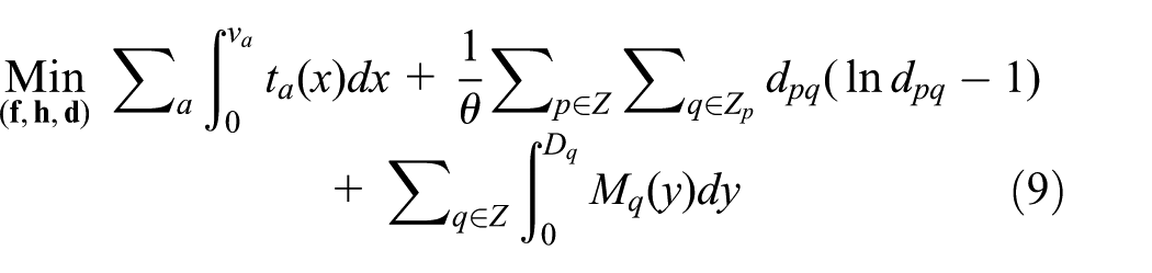


The upper-level problem defines a maximum trip production model. The objective is to maximize the summation of the additional trip production at origins. Equation (5) represents that the traffic flow on every link should not exceed its capacity. Constraints (6) and (7) are the limitation of the zonal trip production and attraction. This means the number of trips generated and attracted at each traffic zone should be limited by some upper bounds, namely
The lower-level problem is the ETDA-VDC model. The objective function (9) indicates the choice behavior of both the existing and additional travel demand. Constraint (11) shows that the amount of the existing flows are fixed for each OD, while constraints (10) and (12) show that the additional flows are only restrained by the origin productions. The relationship between the link flow and route flow is represented in equation (13), where
An sensitivity analysis based solution algorithm
Several solution methods can be used for the network capacity problems. In this study, we present a modified procedure based on the original sensitivity analysis based (SAB) algorithm. 21 The steps of the modified SAB algorithm are given as follows:
Step 0: initialization. Determine an initial value of trip production pattern
Step 1: solving lower-level problem. Solve the ETDA-VDC model in lower level for the given
Step 2: sensitivity analysis. Calculate the partial derivatives,
Step 3: local linear approximation. Formulate local linear approximations of the upper-level capacity constraints using the derivative information, and solve the approximate linear programming problem to produce an auxiliary trip production
Step 4: updating solution. Let
Step 5: convergence criterion. If the convergence criterion is satisfied or the maximum number of iteration is reached, then stop; otherwise, return to Step 1, and set k := k + 1.
Step 1: Route-based algorithm for the ETDA-VDC model
Initialization
Set n := 0, determine the initial link cost
Find the tree of minimum-cost routes rooting from p. For each minimum-cost route
Compute the initial variable OD demands by

For
Update the link costs using the initial link flows.
Main loop
For n = 1 to the number of main iterations (IMain):
1. Equilibrate route flows and retain the additional trip demands. Given the current additional OD demand
For each origin
1.1. Column generation. Update the route cost

Otherwise, tag the minimum route among the routes in
1.2. Shift flow from non-minimum routes to minimum route (a) Compute the route flow shift
where (b) Update the route flows and project it onto the feasible set
If (c) Update the link flows {va}, the link costs {ta}, and the derivative costs


1.3. Compute the new route flow proportions

2. Update OD flows and retain the route flow proportions. Given the route flow proportions 2.1. For each destination zone 2.2. For each OD pair, optimize the additional OD flows as follows: (a) Find the set of auxiliary trip demands
(b) Calculate the auxiliary traffic flow
(c) Let
where (d) Update the link flows and the additional trip demands
2.3. Compute the route flows
2.4. Update the link cost {ta} and the derivative cost


3. Check convergence. Terminate if the convergence criterion is satisfied; otherwise, start a new iteration of the main loop, and set n := n + 1.
Remark 1
The above solution algorithm is developed based on Evan’s algorithm for combined trip distribution and traffic assignment models. The steps are implemented in two stages, in which the trip demand dpq and link flow va are derived in turn. Since the OD demands in the stage for equilibrating route flows vary in each iteration, the route flow proportion
Remark 2
In the proposed algorithm, the route-based method with gradient projection (GP) is used for equilibrating traffic flows. We chose this method because it is easy for obtaining an equilibrated route set which is the necessary prerequisite to use the restriction sensitivity analysis approach in the next step. 22 In addition, the GP algorithm shows good performance for producing high-precision solutions, which is also a necessary requirement for sensitivity analysis. 24
Step 3: Local linear approximation procedure
The bi-level problem is linearized using first-order approximation at the given point,


where

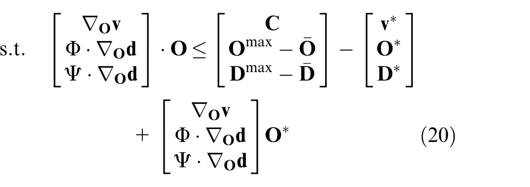
where
Remark 3
The original SAB procedure for the network capacity problem directly uses the solution to the linear approximation as the new start point in the next iteration. According to our tests, the original SAB only works to very small examples. When dealing with larger networks, using the original procedure may conduct an improved solution located outside the feasible region. If the deviation is sufficiently large, a non-solution linearized problem will be formed based on the infeasible point. Considering the linear programming in this step is only a local approximation, the value of the step length should not be too large. Therefore, the maximum step length is adopted to reduce the influence of the approximation errors. In our modified algorithm, the new solution is updated using the convex combination of the solution from the last iteration,
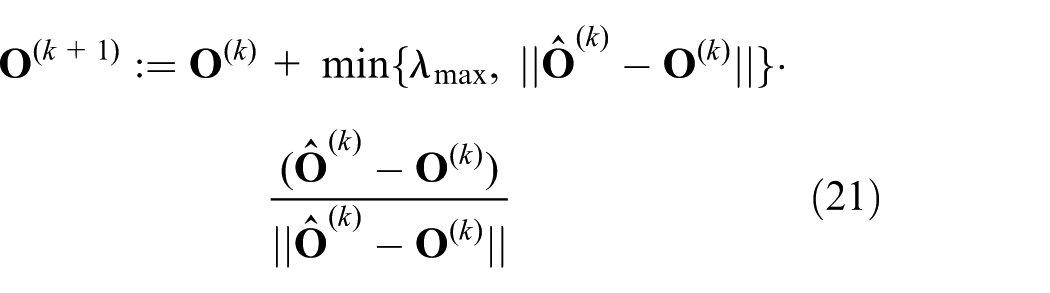
where
Use equation (21) to produce a temporary solution
Solve the lower-level problem based on the temporary origin production
Check the feasibility of the link flows and the zonal trip generations according to the capacity constraints in equations (5)–(7): (a) If the constraints are violated, lower the maximum step length (b) Otherwise, a feasible new point is found, and let
Remark 4
The practical network capacity model is formulated as a non-convex optimization which is hard to solve for a global optimum. In practice, the heuristic methods are usually used to deal with these types of problems. Yang 25 first suggested an iterative estimation assignment (IEA) algorithm in which the derivatives of the decision variables are approximated using the link choice and destination choice probabilities. An efficient method was conducted in Du et al. 26 recently and was shown to find a better solution compared to the original SAB and IEA algorithms. On the basis of our previous research, we further improved the lower-level solution algorithm and adopted a self-adaptive step length restraint. The modified SAB algorithm easily tackles the network capacity problems with larger scale than the previous works.
CNRI
The example in Figure 1 indicates that the NRI may provide a wrong guidance sometimes. The NRI uses the TTT as the evaluation index. The TTT only reflects the transportation efficiency other than the “transportation capacity” of the system. In this section, a new measure, namely CNRI, is suggested which takes the change of the system capacity as an index considering the elimination of the individual link in the transportation network.
Let T be the total capacity of the original network with all full-functional links. Then, Ta represents the capacity of the disrupted network by completely removing link a. So, the CNRI is derived for each link using the decrement in the network capacity when the link is blocked

Thus, the capacity robustness evaluation steps for a transportation network are described as follows, and a flowchart of the procedure is given in Figure 2.
Step 1. Evaluate the transportation capacity of the original network with all links, which produce the value of T. In this study, we employed the practical capacity model to describe the network capacity problem and used the proposed algorithm in the previous section for the model solution.
Step 2. For each individual directed link
Step 2.1. Solve the network capacity problem in the disrupted network where the link a is completely removed, and obtain the value of Ta.
Step 2.2. Compute the CNRI for link a using equation (22).
Step 3. Check if all links in the network have been visited. If not, go to step 2; otherwise, go to the next step.
Step 4. Collect system-wide statistics based on the above evaluation.
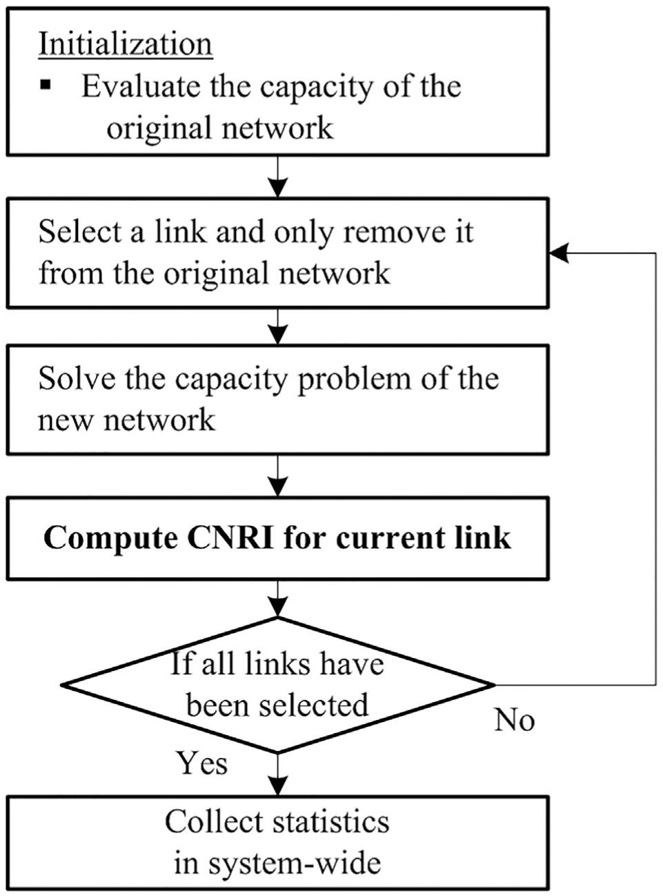
Flowchart of the CNRI evaluation procedure.
Numerical results
A simple example
In this section, we apply the CNRI evaluation procedure to a simple network. The numerical results are produced using the following data:
Test network in Figure 3 consists of 6 nodes, 9 directed links, 2 origins (node 1 and 2), and 2 destinations (nodes 3 and 4).
Link properties are illustrated in Figure 3, and the link travel time function used is the standard Bureau of Public Road (BPR) function:
Existing OD demands are d13 = 18, d14 = 12, d23 = 24, and d24 = 12 (as shown in Figure 3).
Destination cost functions for nodes 3 and 4 are assumed to be
Zonal capacities for the origins and destinations are

Test network.
The CNRI of each link is produced when

Results of the CNRI and NRI for each link.
Figure 5 shows the impact of the impedance parameter (i.e. the dispersion degree of the destination choice behavior) on the results of the CNRI. The impedance parameter θ is given from 0.01 to 10. Note that the overall trend of the CNRI for each link decreases with an increase in the value of the impedance parameter. It means that when the transportation network users are more sensitive to the trip expense, they prefer to choose those closer tourism destinations, and thus the disruption of links could have less influence on the capacity of the whole transportation system. The CNRI of link 1 is shown to be more sensitive to the value of θ, so it is meaningful to predetermine the parameter θ when we apply the proposed CNRI measure.

Impact of the impedance parameter on CNRI.
Sioux Falls network
Comparative experiments are conducted in this section between the CNRI and NRI for network evaluation. For simplification, the destination attractiveness term, Mq, of the travel utility is set to be zero. The results are produced using the following data:
Sioux Falls network comprises 24 nodes, 76 directed links, and 24 origin/destination nodes.
Link properties and travel demand are obtained from Bar-Gera, 27 and the existing OD demand is scaled down from the original data.
Link travel time function employs the BPR function given by
Zonal capacity for each origin or destination is 80,000 unit for both trip production and attraction.
Impedance parameter values are 0.1, 0.2, and 0.5.
The CNRI values are derived under three different values of the impendence parameter, which represent the distinct levels of sensitivity to the travel cost when travelers choose their trip destinations. When θ = 0.2, travelers are not sensitive, and this will produce a scattered trip distribution for the additional demand. As θ = 1.0, the trip distribution is sensitive to impendence, and thus, the distant destinations (with longer travel time) are avoided by travelers. Under different values of θ, the network capacities are evaluated at first. Then, the CNRI values are derived using the modified SAB algorithm. And the NRI is also produced as a reference. Results of CNRI and NRI are summarized in Table 1.
Summary statistics for NRI and CNRI.

NRI: network robustness index; CNRI: capacity-based network robustness index; TTT: total travel time.
According to the base value of the capacity in Table 1, when θ is small, the network generally shows a lower transportation capacity. It is because that more trips with long distance consume most of the resources of the system. In contrast, the capacity could be higher in the cases with larger θ. In Table 1, both the absolute values and the percentage changes from base values are listed. The means of the CNRI values are distinguished and decrease as θ grows. The standard deviations are not very different. The maximum value of CNRI is found when θ = 0.2, for both actual and percentage values. The minimum actual value of CNRI is produced under θ = 1.0, while according to the percentage value, the minimum value of CNRI is detected under θ = 0.2. These give the suggestion that the network with lower value of θ could be more sensitive to the disruption of the links. Note that the network capacity could either increase or decrease for the removal of the individual link. Though the absence of the link may improve the throughput of the network analytically, the system-wide travel time is generally increased according to the corresponding value of NRI.
The comparison of the CNRIs for all links (from link 1 to link 76) is illustrated in Figure 6. Obviously, similar trends are obtained for distinct values of θ in the three cases. For each pair of the three results, a scatterplot of the relationship is shown in Figure 7. A linear or monotonic relationship would suggest that the solutions to critical link identification are similar. The Spearman rank-order correlation coefficient is also computed using the SPSS software. For the three paired comparisons, the correlation coefficients (with p-values in parentheses) are 0.354 (0.002), 0.400 (<<0.01), and 0.278 (0.015), respectively, which means the correlations are significant.
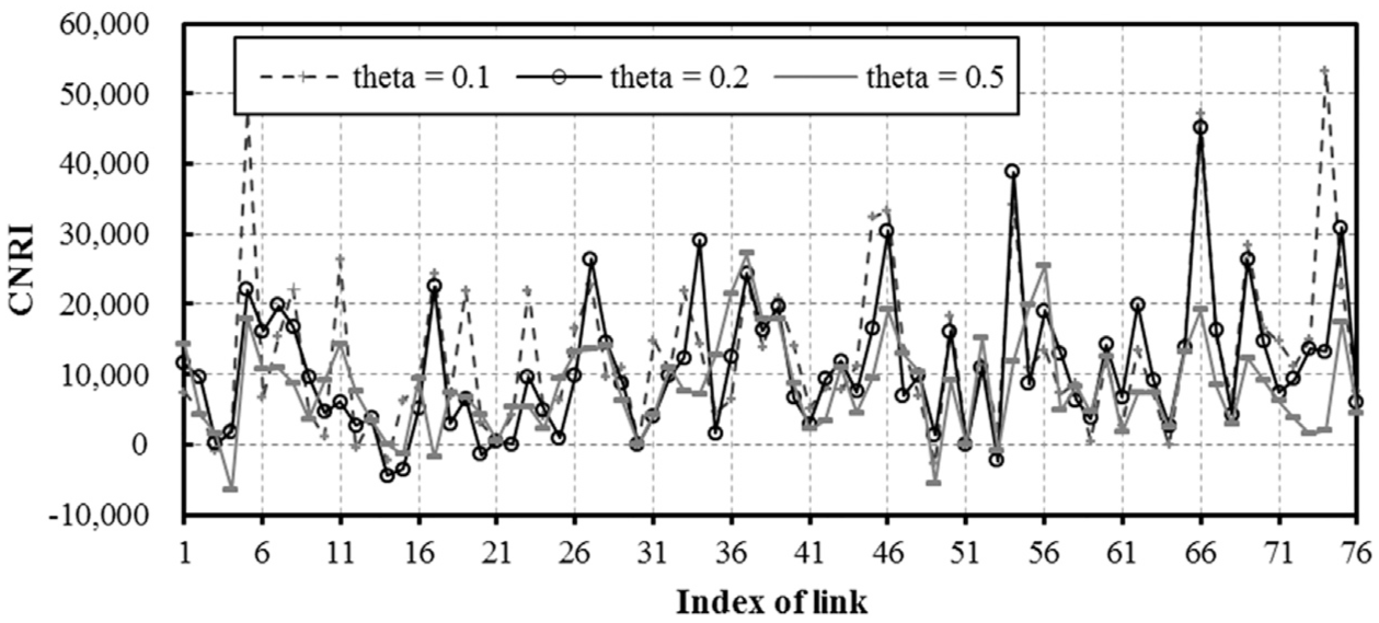
CNRIs of all links in Sioux Falls under different levels of θ.

Relationship among the CNRIs for different levels of θ.
Important differences in the results of critical link identification are reported in Table 2. Table 2 lists the top 10 links (ranked from highest to lowest values) identified according to each measure. There are apparent distinctions among the ranking according to the CNRI and the NRI. For the CNRI, there are four common links (i.e. links 5, 37, 46, and 66) identified in all the three cases; four links (i.e. links 17, 54, 69, and 75) are found twice in the three CNRIs. The results show that if these links are blocked by accidents, destroyed in disasters, or closed for construction, the whole system will lose a significant portion of its capacity for transportation. Compared to the NRI, links 37 and 46 are identified either using the CNRI or the NRI. The total values of the indices in the bottom row are obtained by summarizing the values of the top 10 links identified with deferent measures. The total values show that the transportation networks with lower impedance parameters, θ, are more vulnerable to the network degradation according to CNRI.
Comparative results of critical links by CNRI and NRI (top 10 links).

CNRI: capacity-based network robustness index; NRI: network robustness index.
The bold values signifies that the link is ranked in the top 10 in all three situations with different levels of θ. The italic values signifies that the link is ranked in the top 10 only in two out of three situations.
Besides, the NRI values of the top four links are very close as listed in Table 2. These four links are from two pairs of two-way arcs (i.e. links 16 and 19 connect the same two nodes in contrast directions; same for links 39 and 74). According to the NRI only, the importance of the four links is not clear. Thus, the CNRI can be used as a complement for making decision. For example, according to the CNRI, when θ = 0.2, the rank order is CNRI39 > CNRI74 > CNRI19 > CNRI16. Hence, the importance of the links can be distinguished well. In such situation, the CNRI could be used as an efficient alternate measure in transportation network evaluation.
Conclusion
This study proposed a novel index to evaluate network robustness of transportation system. The new measure was formulated based on the well-known practical network capacity model. The proposed CNRI was represented by the variation of the total capacity of the transportation system when a single link is completely blocked. Differing from the NRI which utilizes the travel time as the indicator, the CNRI is supposed to be more straightforward to reflect the impact on the system-wide transportation ability. A counter-example was also presented to show the effectiveness of the CNRI. According to the numerical experiments, the CNRI provides distinct solutions to the critical link identification compared to the NRI approach. The comparison also showed that the CNRI can give useful complementary information when the results from the NRI are not significant. The CNRI is suggested to be a necessary option to detect the robustness of transportation system. These conclusions were conducted on the Sioux Falls test network. Future research will focus on the practical applications of the CNRI using real transportation networks. Besides, more characteristics could be studied using different network capacity models with various travelers’ choice behaviors.
Footnotes
Academic Editor: Hai Xiang Lin
Declaration of conflicting interests
The author(s) declared no potential conflicts of interest with respect to the research, authorship, and/or publication of this article.
Funding
The author(s) disclosed receipt of the following financial support for the research, authorship, and/or publication of this article: This research was supported by the National Natural Science Foundation of China (nos 51408190, 51508161, and 71501061), the Natural Science Foundation of Jiangsu Province (nos BK20150817 and BK20150821), and the Fundamental Research Funds for the Central Universities (no. 2014B04514).