New design method for horizontal alignment of complex mountain highways based on “trajectory–speed” collaborative decision

Abstract

The safety evaluation of geometry features design based on actual driving behavior has always been a basic concept of highway design. However, current design methods, including both the design speed method and operating speed method, are still far away from real-world driving conditions. In this work, we propose a new alignment design method which can take into account typical handing patterns (driving styles) of human drivers and can pay special attention to dangerous driving behaviors. The core of the proposed method is forecasting the trajectories of typical direction control patterns within roadway width, which can be used by drivers. Then, forecast the driving speed of typical speed control patterns on the basis of the curvature of the preview trajectory just determined. Mathematical programming method was used in this study, whereby the objective functions and constraints were developed to model the typical driving patterns. This article provided five direction control patterns and four speed control patterns to designers so that they could select an appropriate pattern to predict the trajectory and speed for the designed road. Finally, the trajectory and speed are used to control the geometric features of the road. Geometric features can determine the driveway shape, such as curve radius, deflection angle, spiral length, tangent length, roadway/lane/shoulder width, and any or all of these can be adjusted by the designer. Meanwhile, as more than one driving pattern is optional and vehicle performance, driving stability, and ride comfort restrictions are introduced to trajectory/speed decision-making, the new method more closely approximates to real-world driving than conventional methods. The application example shows that the proposed method is especially suitable for the horizontal alignment design of low/medium design speed highways that traverse rugged terrain.

Introduction

Modern highways are designed primarily for use by motorized vehicles. Therefore, design theory and methodology applied to highway alignment should be able to support modern vehicle performance and to satisfy the driving habits of users. ¹ Unlike train drivers who must operate their vehicles in strict accordance with operational diagram, automobile drivers have the freedom to choose their trajectory and speed. ² For example, in curved mountain roads, many different direction control patterns can be observed. These include curve cutting, centering in the lane, driving around the outside or the inside of a curve, and encroaching onto the shoulder. At the same time, drivers exhibit different speed control habits such as traversing a curve at high speed (only slowing slightly), slowing down sharply through a curve, and traversing a curve at a constant low speed. Therefore, in reality, driving behavior exhibits characteristics of diversity and differentiation.

To enable actual driving reflected in highway design, the alignment/geometry design methods adopted around the world have been modified many times over the past several decades. In spite of this, these methods are still far away from the principle of “applying actual driving behavior and vehicle performance to highway geometric design.” The design speed assuming “drivers drive on highways at the constant design speed” is still the controlling variable when defining the horizontal and longitudinal alignment element values. Design policies of different countries differ in whether to use the operating speed when conducting a safety evaluation.^3,4 Furthermore, all previous revisions of design specification have not reflected the important role of the drivers’ direction control behavior (shown as the trajectory characteristic) although there is a close correlation between the trajectory and speed, which is manifested as different trajectory control habits inevitably corresponding to different speed selection behaviors. ⁵ On the other hand, the trajectory shape and topology can exert a direct control effect on both the horizontal alignment and cross-sectional design. ⁶ Because these factors are not considered, conflict between the highway design and driver behaviors will often appear, leading to frequent accidents. Obviously, the inherent defects in the design theory must take some responsibility for many crashes. ⁷

This article proposes a horizontal alignment design method for mountain highways that considers the typical driving patterns when human driver selected their target trajectory and speed. Using this method, trajectories of typical driving patterns are determined within the available pavement width, after which the driving speed is determined using the curvature of the determined trajectory. Therefore, any change in the geometry features such as radius, deflection angle, spiral, road width, length of tangent, curve deflection direction, and obstacles on road surface will affect the trajectory shape, this will inevitably be reflected in a change in the driving speed. Therefore, through cooperative control of “trajectory–speed,” the designer can evaluate and adjust more geometric elements and thus provide high-quality highway alignment that can fit with the natural driving habits of human drivers.

Literature review

The proposal of a new design method has been prompted primarily by the fact that the current methods neither satisfy the needs of road users nor meet the designer’s expectations. Thus, prior to presenting the method proposed herein, it is necessary to make a comparison with and analysis of current highway alignment design methods. Given that the US popularized the use of the automobile, the highway design methods adopted by countries around the world have mostly been based on the design speed method put forward by the American Association of State Highway and Transportation Officials (AASHTO) in 1938. ¹ At that time, road users did not know enough about vehicle performance and mostly lacked adequate driving experience which, when combined with poor road conditions poor performance of vehicles, made driving speeds generally slow. Thus, AASHTO defined the “design speed” as “the maximum approximately uniform speed which would probably be adopted by the faster group of drivers but not, necessarily, by the small percentage of reckless ones.” This definition remained in use until the fourth revision in 1954. Driving speeds have greatly increased owing to significant improvements in vehicle design and manufacturing technologies over the decades, which leading to the effect of road geometric factors on vehicle speeds becoming a major issue, in response to this, road design theory has also been improved. Therefore, in that revision, the design speed was defined as “Design Speed is a speed determined for design and correlation of the physical features of a highway that influence vehicle operation. It is the maximum safe speed that can be maintained over a specified section of highway when conditions are so favorable that the design features of the highway govern.” That is, in essence, it is the critical safe speed through difficult road sections. This definition remained in effect until the seventh revision in 1977. Over the past 20 years, the number of motorized vehicles in the United States has continued to increase, first leading to traffic jams in urban streets, and then expanding to trunk roads. Therefore, the restricting condition of “on a highway in ideal weather and with low traffic (free-flowing) conditions” was added to the definition to eliminate the interference arising from traffic jams. Also, in the 1970s, some scholars in Europe and America conducted extensive observations of highway driving speeds and discovered that the statement was not in fact rigorous, especially given the great discrepancy between the description of “a nearly consistent maximum or near-maximum speed that a driver could safely maintain on the highway” and the reality occurred in highway. Therefore, in the 2001 revision, the definition of the design speed was revised to “The Design Speed is a selected speed used to determine the various geometric design features of the roadway.”

When using such a classical design method, designers use the selected design speed V_d to determine the minimum radius of a horizontal curve, the super-elevation rate, sight distance, gradient, length of grade, and lane width, where the sight distance requirement can also be used as control parameter for the radius of a vertical curve. ⁸ At present, countries adopting the design speed method include the United States, Canada, Belgium, South Africa, China, Japan, and so on.

The design speed method simplifies the complicated and uncertain process of driving along a road into a certain problem, that is, “drivers steering their cars so as to track the centerline of the roadway at a constant speed equal to the selected design speed.” In reality, however, drivers select their target trajectory and speed based on the geometric features of the road, pavement conditions, operating status of the automobile, and personal physiological feelings. Especially when driving on a mountain road, the geometric features and available roadway for a driver change greatly along the route, which causes the trajectory and speed to change significantly along the distance traveled, while the diversity of the personal behaviors between different drivers also contributes to these changes. For example, unlike the constant or nearly constant driving speed adopt by drivers when traveling on expressways, as shown in Figure 1, the dramatic changes in driving speed of passenger cars measured on two-lane mountain roads can be seen in Figures 2 and 3, where the continuous speed of passenger cars was measured under free-flow conditions. The peak values of the speed profiles in Figures 2 and 3 are about twice V_d, and the minimum speed is lower than V_d, which indicates that for roads in mountainous regions, it is hard for designers to provide drivers with a driving environment that is consistent with the design speed. Since there is a very large difference between V_d and the actual speed, the super-elevation and sight distance determined by V_d do not coincide with the actual requirements of a moving vehicle.

Figure 1.

Driving speed of a passenger car measured on a four-lane expressway: (a) horizontal alignment and (b) measured speed of passenger car.

Figure 2.

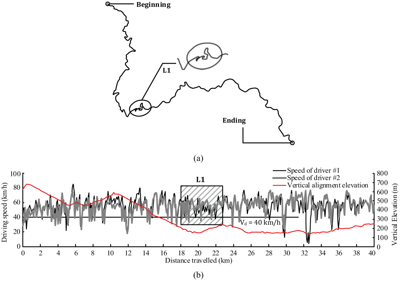
Alignment and driving speed of a province road section with design speed of 40 km/h: (a) horizontal alignment and (b) measured speed and vertical alignment elevation.

Figure 3.

Driving speed measured on a 25 km section of a province road with a design speed of 30 km/h: (a) horizontal alignment and (b) measured speed and vertical alignment elevation.

Moreover, by observing the speed profiles of two-lane mountain roads, for passenger cars, the change in the horizontal alignment remains the leading factor causing operating speed fluctuations, since no relationship between the speed and grade can be observed in these two figures. This shows that on mountain highways with long and steep downgrades, the main task of the drivers is still to deal with steering to keep their cars in the lane while adjusting their speed to safely negotiating the sharp curves. Therefore, on two-lane highways through mountainous regions, the horizontal alignment and cross section are factors affecting the speed of a passenger car, but the vertical alignment has almost no influence.

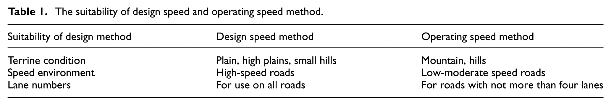
The operating speed method solves these problems brought by design speed method effectively. ⁹ Since the 1970s/1980s, some countries, such as Germany, Britain, France, Switzerland, Spain, and Australia, have begun to realize the disadvantages of the design speed method and have been gradually improving it so as to establish an operating speed method that is a reasonable approximation to the actual driving conditions. The operating speed is the speed at which a vehicle is driven under free-flow conditions and is obtained using certain observation means, often expressed with the 85th measured speed at the observation position, that is, V₈₅. The predicting models of operating speed, using geometric features as the independent variable, are often obtained through a regression analysis of the observation data. Designers substitute the element values of the initially proposed alignment in sequence along the roadway to obtain a profile of the operating speed, which can be used to control the smooth transition of the index value of adjacent alignment elements, and thus guarantee the consistency of the geometric design. Furthermore, V₈₅ can also be used to determine or check the super-elevation rate and sight distance. ¹⁰ However, in design practice, a nominal design speed is generally necessary to control the maximum or minimum values of geometric elements. Table 1 summarizes the suitability of these two design methods for road geometry.

Table 1.

The suitability of design speed and operating speed method.

Suitability of design method	Design speed method	Operating speed method
Terrine condition	Plain, high plains, small hills	Mountain, hills
Speed environment	High-speed roads	Low-moderate speed roads
Lane numbers	For use on all roads	For roads with not more than four lanes

The prediction models of V₈₅ are the core of the design method based on operating speed; in the last three decades, lots of V₈₅ models have been proposed by researchers from different countries and regions. Three-dimensional (3D) road surface can be decomposed into horizontal, vertical, and cross-sectional components. The horizontal alignment can be further decomposed into straight, spiral, and circular components. Most existing models have been developed for a specific type of road section or single/multiple geometric elements. Operating speed models currently in use include horizontal circular curve models,^11,12 straight road models, ¹³ curved slope models,^14,15 desired speed models, ¹⁶ roadside interference models, ¹⁷ and traffic impact models. ¹⁸ In addition to these models, Russo et al. ¹⁹ developed a predicting model to be used at the same time on tangents and circular curves.

Limitations in operating speed method

Compared with the design speed method, an improvement in operating speed method is that the influences of the geometry features on driver behavior can be reflected in highway design, as a result the super-elevation rate and the sight distance determined by V₈₅ are more reasonable, and the consistency of highway alignment is improved by controlling the difference between the radii of adjacent curves. However, based on the mass measurement data of driving behavior over mountain highways and discussions with practitioners, we believe that the operating speed design method currently used incurs the following disadvantages.

Geometric features adjustability is very limited

Since consistency evaluation and design improvement of the geometric features are conducted based on the V₈₅ profile, only those road variables incorporated into the V₈₅ model can be adjusted. However, the current V₈₅ model is specific to horizontal curves and the most commonly used variable that it incorporates is the curve radius R or the variation of R, such as the curvature change rate (CCR) and the degree of curvature (DC). ²⁰ In fact, elements such as deflection angle, roadway width, and spiral length can influence the speed choice behavior of drivers.

Interaction between adjacent curves is not taken into consideration

The current V₈₅ model for horizontal curves relates only to a single curve. This is acceptable for a highway crossing smooth terrain, since there is often a long tangent between two adjacent curves. However, for highways crossing rugged terrain, since the tangent between two adjacent curves is either short or not present at all, there is very obvious coupling between the adjacent curves in terms of driving behavior. As shown in Figure 4, the trajectory and speed selection behavior of drivers on curve C_i is influenced by its succeeding curve C_i + 1, and the trajectory and speed on C_i will change if the deflection angle, radius, and deflecting direction of C_i + 1 change.

Figure 4.

Influence of adjacent curves on vehicle trajectory: (a) trajectory through successive curves, (b) curvature of road centerline and trajectory, and (c) simulated speed and measured speed.

The assumption of speed changes within curve areas is unreasonable

Operating speed determined by the existing V₈₅ models is a constant value within the scope of a circular curve, which is equivalent to assumption that drivers negotiate a circular curve at a constant speed. On the other hand, there are two methods of handling a speed change at the entry to and exit from a circular curve: the first involves the assumption that drivers complete their speed adjustment on the spiral. ²¹ The second involves calculating the acceleration and deceleration distances based on a predefined acceleration rate. ¹¹ However, driving at a constant speed through a circular curve as assumed is not actually found from the measured speed for single vehicles; on the contrary, the deceleration behavior of drivers often continues into the circular, with the acceleration being reapplied after the lowest speed is reached. This is because drivers adjust their speed based on the trajectory curvature or the centrifugal force when driving around a curve, that is, accelerating when the centrifugal force decreases, and decelerating when the force increases. However, the trajectory curvature is not consistent with the horizontal curvature of the road. As shown in Figure 5, drivers can select a large trajectory radius within the roadway to reduce the discomfort when negotiating the curve. Trajectory adjustment begins before the curve entry to achieve the aim so that the start point for negotiating a curve is prior to the point TS, and a trajectory curvature peak appears in the middle of the curve.

Figure 5.

Trajectory shape and curvature when negotiating a curve: (a) trajectory when a vehicle negotiates a curve, (b) curvature of road centerline and trajectory, and (c) simulated speed and measured speed.

Insufficient consideration of direction control behavior (trajectory characteristics)

Both the design speed and operating speed methods take the curve radius R as a parameter for calculating the sideways force coefficient of a vehicle, that is, a design principle of “assuming the centerline of the road as the vehicle trajectory” is adopted. However, on an actual highway, different patterns of trajectory selection behaviors can be observed, and the above assumption is only suitable for those drivers whose habit is to keep their vehicle in the middle of the lane, KVMD. However, our observations show that the average occurrence of KVMD is less than 8% (the value quoted by Spacek ⁵ is less than 2%), while curve cutting appears to be the most common behavior on mountain roads. Therefore, when determining the values of the alignment parameters in highway design, we should consider all typical driving habits while paying special attention to the most common driving habits to increase the tolerance for error. The advantages of taking the trajectory radius as the basis for calculating the geometry parameters are clear from Figure 6. At present, the width of a standard lane in China is 3.00–3.75 m, while the shoulder width is 0.5–1.5 m. Considering the habit of drivers who encroach into the opposite lane by 0.5–1 m when the traffic flow is low, the pavement width available to drivers is generally 4.25–6.25 m, which indicates that drivers have ample opportunities to select their preferred trajectory. From figure 6, it can be seen that the trajectory radius R_t when driver cutting the curve is obviously higher than R, and the wider the lane, the greater the difference between R_t and R.

Figure 6.

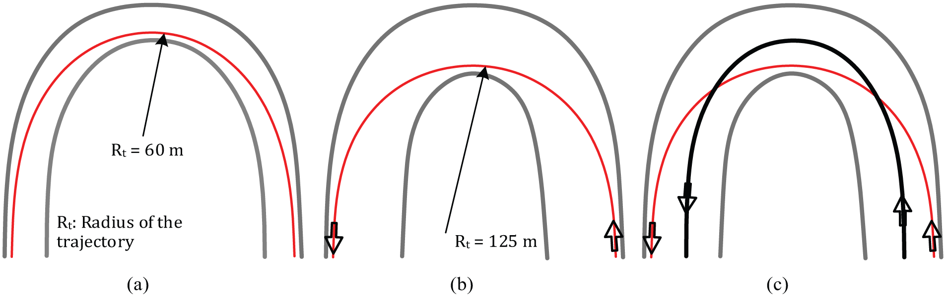
Difference between trajectory radius and curve radius: (a) available pavement width is 4 m, driver cut the curve; (b) available pavement width is 6 m, driver cut the curve; and (c) driver cutting the curve reaches the curve exit more quickly than when following the curve.

New design methods of horizontal alignment

Design concepts

There must be a design concept which supports the use of a certain design speed method. We can conclude that the design concept of the design speed method involves

assuming that drivers control their vehicles to track the centerline of the road while maintaining their speed at a constant amplitude (the design speed), and then determining the values for the geometric features of the roads based on the design speed.

This design concept is well-suited to the driving characteristics of a high-speed environment, so it is ideal for the design of high-grade highways over smooth terrain.

For lower-speed expressways (Vd 80 km/h) through mountainous areas, as well as two-lane mountain highways, the design speed method obviously becomes less applicable or even invalid since the driving conditions are fundamentally different. The operating speed method based on the design concept of

Drivers controlling their vehicles to track the centerline of the road and changing their speed based on approaching road geometry features, and then determining the values for the geometric features of roads based on V₈₅.

can be adapted to highway alignment design in intermediate- and low-speed driving environments to a certain extent, since it reflects the influence of the road geometry on the speed selection behavior of drivers.

However, there remains a great difference between operating speed design concept and actual driving characteristics. The selection of a desired speed by a driver in the real world mainly depends on the curvature of their preview trajectory, as the geometry features including the deflection angle, spiral, available pavement width, horizontal curve length, deflection direction, and tangent length can all affect the shape of the road in front, and thus furthermore affect the curvature of target trajectory. The trajectory shape and its curvature are also influenced by the driver’s habits and the vehicle’s characteristics. To apply such factors to the geometric design of roads, the design concept of

considering the natural driving habits of human drivers, predicting the trajectory of typical direction-control patterns within the pavement width that can be used by a driver, predicting the speed corresponding to typical speed-control patterns based on the trajectory curvature under the constraints of the dynamic properties of a vehicle, driving safety, and comfort, and thus determining the values for the geometric features of a road using the trajectory and speed of the selected driving pattern

is adopted as the new design method proposed in this article. The change in design concept of highway alignment is illustrated in Figure 7.

Figure 7.

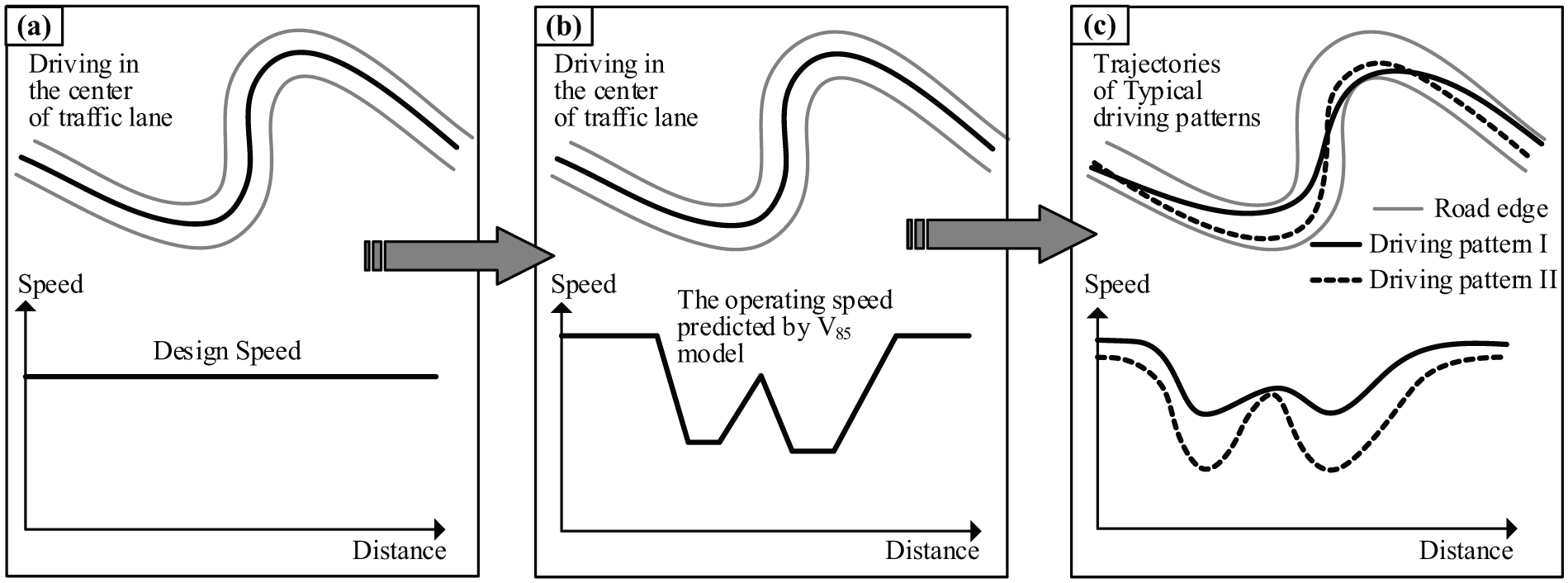
The change of the design concept of highway alignment: (a) the concept of design speed method, (b) concept of operating speed method, and (c) the concept of the new method proposed in this study.

Implementation technology

Two key problems need to be solved to complete the transformation from a design concept to a technological means that can be directly applied to highway alignment design: the first is that when the initial alignment and design vehicle are given, how to predict the trajectory of typical driving patterns within the boundaries of driveway; the second is how to predict the speed of the selected driving patterns based on the curvature characteristics of the predicted trajectories. These two technical issues were solved in our prior works.^22,23 How to link the two methods of trajectory decision and speed decision and the resulting global properties after the linking are described in the following.

Calculation strategy of “trajectory–speed” coupling

We adopted the parallel calculation process shown in Figure 8 for trajectory–speed decision, where the “trajectory” is the vehicle path on the designed road corresponding to a selected driving pattern of direction control, the “speed” is the velocity of the vehicle corresponding to a selected driving pattern of longitudinal control when following its path. In this study, trajectory decision and speed decision are intercrossed and interactional, which confirms the actual highway driving process. For example, when a vehicle is approaching a small-radius curve with a good sight distance, the driver can obtain a large trajectory radius by cutting the curve to negotiate it at a higher target speed, and the driving speed will increase accordingly if the centrifugal force decreases when around the curve owing to the flattened trajectory.

Figure 8.

Process for determining trajectory and speed.

The study presented a strategy of “selecting a trajectory point on a preview cross section within driver’s sight-window” for trajectory decision-making, as shown in Figure 9(a). Cross sections perpendicular to the direction of travel are marked within the driver’s sight window in front of the vehicle at specific intervals to create a set of candidate trajectory points, and then the trajectory choice behavior of a driver is simulated by sliding the point P_ti on the preview cross section P_liP_ri. For cross section P_liP_ri, a proportionality coefficient $S_i\in [0,1]$ is used to describe the movement of P_ti mathematically, as shown in Figure 9(b) and (d), where S_i → 0 indicates the trajectory point sliding toward the right. Since the two endpoints of a cross section can be obtained analytically for a given roadway, once S_i is solved, the position of P_ti can be determined. Therefore, the trajectory decision-making is in essence the process of determining variable {S_i| i = 1∼n}. Since a change in the position of P_ti will lead to a change in trajectory length, trajectory curvature, sideway force coefficient, and so on, adding these parameters to the objective functions and constraints can realize the simulation of a driver’s trajectory selection behavior.

Figure 9.

(a) “Trajectory–speed” calculation strategy: (1) drawing preview cross sections; (2) selecting a point on a preview cross section within the sight window; (3) rolling the sight window; (4) linking adjacent trajectory points; (5) calculating the curvature of the trajectory; (6) calculating the acceleration rate and then optimizing it; (7) desired speed decision-making. (b) Implication of proportionality coefficient S_i. (c) Illustration of constraint of roadway geometry on target trajectory selection. (d) Mathematical description of the trajectory.

The trajectory curvature K_i is determined at point P_ti after obtaining the target trajectory, then served as the input data for the speed decision in the format of (L_ti, K_i), where L_ti is the spacing between two neighboring trajectory points. Then, a decision variable V_i is set on each cross section, that is, the target speed. The expressions for the travel time t_i and longitudinal acceleration a_xi between any two adjacent cross sections can be constructed using L_ti and V_i, and the expression for the lateral acceleration a_yi can be constructed using K_i and V_i. The objective functions and constraints can be developed using t_i, a_xi and a_yi. Threshold values are set based on the performance of the selected vehicle and the tolerance of the driver, and then using a rolling horizon algorithm to determine the optimal value of the selected objective function that corresponds to a driving habit.

Decision model for trajectory and speed

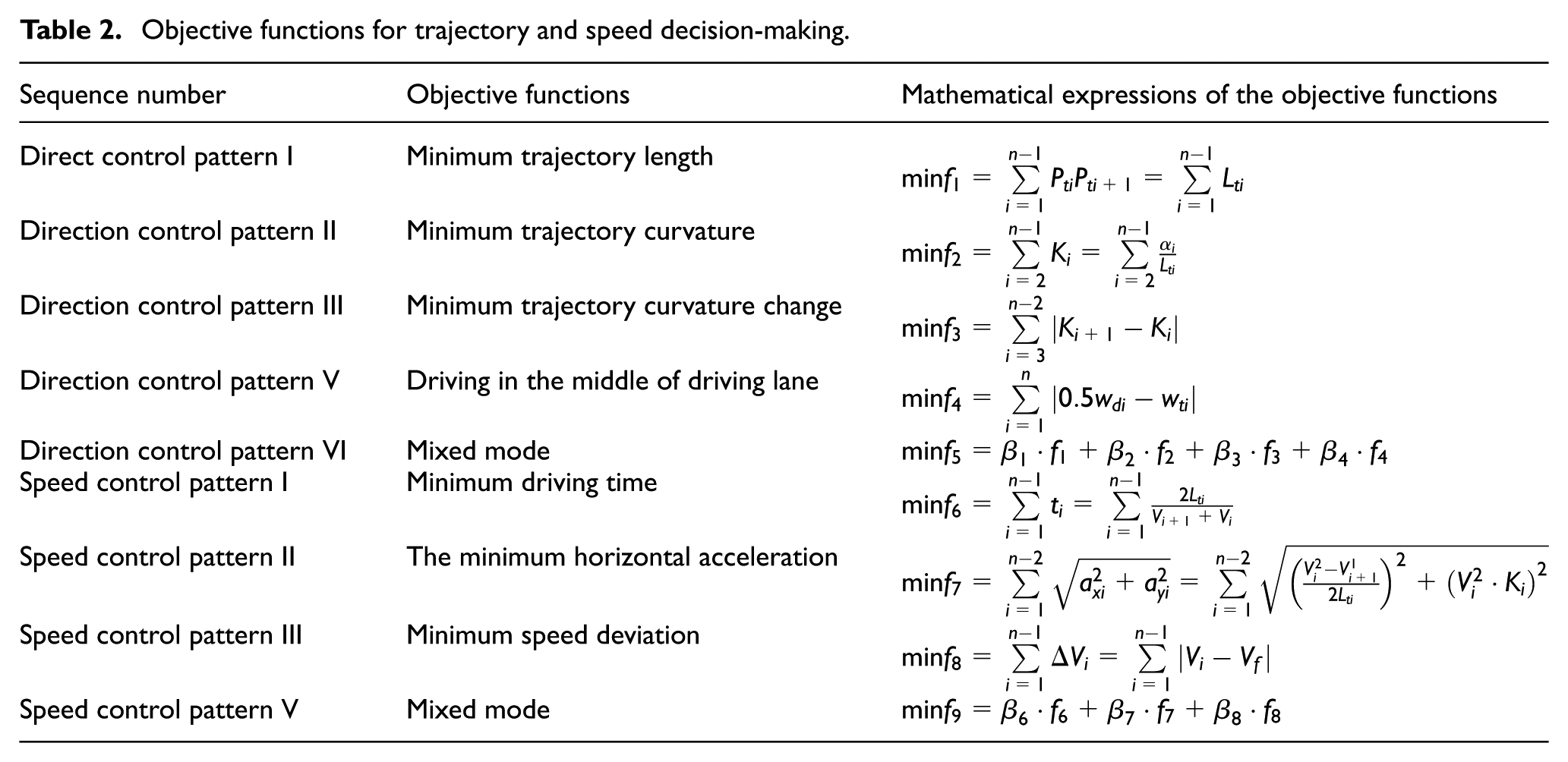
Since the trajectory and speed are calculated using the method of mathematical optimum, how to reflect driver behavior, environment, vehicle performance, and driving characteristics on the objective functions and constraints becomes very critical. Table 2 shows the objective functions corresponding to typical direction control patterns and typical speed control patterns derived from human drivers. Table 3 shows the constraints in “trajectory – speed” decision models. Refer to the research^22,23 for details of the rolling horizon algorithm used to determine decision variables S_i and V_i.

Table 2.

Objective functions for trajectory and speed decision-making.

Sequence number	Objective functions	Mathematical expressions of the objective functions
Direct control pattern I	Minimum trajectory length	$\min f_1=\sum _{i=1}^{n-1}{P}_{\mathrm{ti}}{P}_{\mathrm{ti}+1}=\sum _{i=1}^{n-1}{L}_{\mathrm{ti}}$
Direction control pattern II	Minimum trajectory curvature	$\min f_2=\sum _{i=2}^{n-1}{K}_i=\sum _{i=2}^{n-1}\frac{{\alpha }_i}{L_{\mathrm{ti}}}$
Direction control pattern III	Minimum trajectory curvature change	$\min f_3=\sum _{i=3}^{n-2}|K_{i+1}-K_i|$
Direction control pattern V	Driving in the middle of driving lane	$\min f_4=\sum _{i=1}^n|0.5w_{\mathrm{di}}-w_{\mathrm{ti}}|$
Direction control pattern VI	Mixed mode	$\min f_5={\beta }_1·f_1+{\beta }_2·f_2+{\beta }_3·f_3+{\beta }_4·f_4$
Speed control pattern I	Minimum driving time	$\min f_6=\sum _{i=1}^{n-1}{t}_i=\sum _{i=1}^{n-1}\frac{2L_{\mathrm{ti}}}{V_{i+1}+V_i}$
Speed control pattern II	The minimum horizontal acceleration	$\min f_7=\sum _{i=1}^{n-2}\sqrt{a_{\mathrm{xi}}^2+a_{\mathrm{yi}}^2}=\sum _{i=1}^{n-2}\sqrt{{\left(\frac{V_i^2-V_{i+1}^1}{2L_{\mathrm{ti}}}\right)}^2+{(V_i^2·K_i)}^2}$
Speed control pattern III	Minimum speed deviation	$\min f_8=\sum _{i=1}^{n-1}\Delta V_i=\sum _{i=1}^{n-1}|V_i-V_f|$
Speed control pattern V	Mixed mode	$\min f_9={\beta }_6·f_6+{\beta }_7·f_7+{\beta }_8·f_8$

Table 3.

Constraints for trajectory and speed decision-making.

Serial number	Constraint condition	Mathematical expressions of constraints
Trajectory constraint I	Roadway geometry constraint	$\mathrm{S}.\mathrm{t}\frac{w_b}{w_{\mathrm{di}}}\le S_i\le \frac{1-w_b}{w_{\mathrm{di}}}$
Trajectory constraint II	Rolling stability constraint	$\mathrm{S}.\mathrm{t}{K}_i<0.5·g·\frac{L_b}{V_i^2·H}$
Trajectory constraint III	Side-slipping stability constraint	$\mathrm{S}.\mathrm{t}{K}_i<g·\frac{f_r+h}{V_i^2}$
Trajectory constraint IV	Curve traffic-ability constraint	$\mathrm{S}.\mathrm{t}{R}_i=\frac{1}{K_i}>R_T$
Trajectory constraint V	Obstacle avoidance constraint	$\mathrm{S}.\mathrm{t}{S}_i<\frac{w_b+w_1}{w_{\mathrm{di}}}$
Speed constraint I	The maximum/minimum speed constraint	$\mathrm{S}.\mathrm{t}{V}_{\min }<V_i<V_{\max }$
Speed constraint II	Lateral stability constraint	The same as the second and the third of trajectory constraints
Speed constraint III	Longitudinal dynamics constraint	$\mathrm{S}.\mathrm{t}{a}_{b\max }<a_{\mathrm{xi}}<a_{x\max }$
Speed constraint IV	Longitudinal comfort constraint	$\mathrm{S}.\mathrm{t}{a}_{\mathrm{btol}}<a_{\mathrm{xi}}<a_{\mathrm{xtol}}$
Speed constraint V	Lateral comfort constraint	$\mathrm{S}.\mathrm{t}{a}_{\mathrm{yi}}<a_{\mathrm{ytol}}$

In Tables 2 and 3, L_b is the wheelbase, H is the height of the gravitational center of the automobile, f_r is the friction coefficient of the pavement, h is the super-elevation rate of a horizontal curve, R_T is the turning radius of the automobile, w₁ is the width of an obstacle on the road surface, V_f is the target cruising speed, V_max is the maximum speed of travel, V_min is the minimum speed of travel, a_bmax is the maximum braking deceleration, a_xmax is the maximum longitudinal acceleration, a_btol is the tolerable braking deceleration, a_xtol is the tolerable longitudinal acceleration, a_ytol is the tolerable lateral acceleration, and β_i is the weighting coefficient. In the objective functions, L_ti = ((x_ti + 1 − x_ti)² + (y_ti + 1 − y_ti)²)^0.5, $x_{\mathrm{ti}}=x_{\mathrm{ri}}+w_{\mathrm{di}}·S_i·\cos {\theta }_i$ , $y_{\mathrm{ti}}=y_{\mathrm{ri}}+w_{\mathrm{di}}·S_i·\sin {\theta }_i$ , K_i is the curvature of the trajectory at point P_ti.

Vehicle factors in “trajectory–speed” decision models

Trajectory and speed are used to describe the movement of a vehicle when it is traveling on a roadway. They are the response of the vehicle’s systems to the driver’s operational inputs, so vehicle performance factors will certainly have an influence on the kinematic behavior and will result in different trajectory and speed characteristics. During actual driving, the influence of vehicle performance is mainly reflected in the limitations of the kinematic behavior of the vehicle, so it can be described with constraints, as follows:

Vehicle acceleration performance

Acceleration ability directly determines the change rate while a driver is speeding. There is a clear difference between the different types of vehicles in terms of the ratio of vehicle mass to engine power, and this difference is reflected in the greater sprung mass, the poorer acceleration in the dynamic characteristics. Field observations show that vehicle acceleration ability increases from low to high in the order of heavy trucks, medium-sized trucks, large buses, medium-sized buses, light trucks, minivans, and then cars. According to the measurements obtained from two-lane mountain highways, in Table 3, a_xmax takes value of 0.408–1.964 m/s², with an upper limit for cars, a lower limit for heavy trailers with more than five axles, and the values for other vehicle types being taken within the range based on the sprung mass of the vehicle.

Vehicle braking performance

A vehicle’s braking performance and stability with normal pavement conditions are also closely related to the sprung mass. According to measured values on two-lane mountain highways, in Table 3, a_bmax takes a value of 0.548–2.539 m/s². Therefore, a suitable value should be selected from this range based on the ratio of the vehicle mass to the engine power, and then added to the corresponding speed constraints.

Curve traffic-ability

For two-lane roads through mountainous areas with lower technical standards, a horizontal curve with a small radius shall be checked to determine whether it satisfies the traffic-ability requirement for overlong vehicles, such as a semi-trailer with five or more axles so that the constraint for traffic-ability on sharp curves is set, that is, the trajectory radius shall be greater than the minimum turning radius of the vehicle R_T.

Side-slipping stability

This constraint applies to passenger cars with a low center of gravity, requiring a sideways force coefficient of a moving car below the pavement friction coefficient f_r. It can be used for determining both the trajectory and speed. When used to determine the trajectory, the expected speed V_i is the known parameter; when used to determine the speed, the trajectory curvature K_i is the known parameter.

Rolling stability

In the same way as for the side-slipping stability, this constraint can also be used for determining both the trajectory and speed. It requires that a moving vehicle remaining upright, so it is mainly specific to vehicles with high centers of gravity, such as heavy trucks and large coaches. Before a trajectory decision or speed decision is made, the height of the center of gravity H and the wheelbase L_b shall be substituted into the constraints listed in Table 3.

Environment factors affecting “trajectory–speed” decision models

Since the behavior of drivers is obviously influenced and restricted by the road environment when they steer their vehicles along a highway, we set the following four constraints to simulate these influences:

Roadway boundary

Remaining the vehicle within the available pavement width can be used by a driver shall certainly be guaranteed during trajectory decision-making. Given this constraint, the boundary of the roadway may be set flexibly based on the actual situations, and may be the curb edge, driving lane edge, shoulder edge, or another line, depending on available roadway width.

Maximum and minimum speed

The maximum speed V_max of a passenger travel on an actual highway is restricted by various factors. Under conditions of free-flowing traffic, V_max on normal and smooth pavement is mainly affected by the geometric features of the roadway, such as lane width, shoulder width, total pavement width, and the average curvature of the horizontal alignment. These factors are all related to the technical grade of the highway. Table 4 lists the values of V_max obtained from the measured results for more than 70 highways of different types, where V_max,p and V_max,b are the values for passenger cars and large buses, respectively. Since there are many combinations of axle number and sprung weight of freight vehicles, a unified value of V_max may be difficult to set. Alternatively, users can set their own threshold values according to the vehicle being analyzed. The minimum speed V_min on a highway under free traffic flow often occurs on difficult road sections such as sharp curves, steep grades, and combinations thereof, and the geometry feature values for such difficult sections are usually determined by the design speed V_d. According to the measured value on highways, 0.7 times V_d is taken as the value of V_min in the constraints.

Table 4.

Maximum speed of travel measured on different types of highway (km/h).

Design speed	Six-lane highway		Four-lane highway					Two-lane highway					One-lane highway
	120	100	Expressway			First-class		80	60	40	30	20	20
			100	80	60	80	60
V max,p	145	135	130	110	90	110	90	115	105	88	78	70	60
V max,b	120	100	100	90	80	90	70	90	75	60	50	40	30

Obstacle avoidance

The appearance of an obstacle on the roadway will lead to a change in available pavement width in front of the vehicle. With this feature, the mathematical description of obstacle avoidance can be provided, that is, it is only necessary to substitute the width of obstacles such as roadside parking, bicycles, pedestrians or a closed lane w₁ into the constraints before starting a simulation of determining a trajectory and speed.

Driver factors in “trajectory–speed” decision models

Natural driving patterns

Drivers control the movement of their vehicles (which can be described by the trajectory and speed) over the road through their operational behavior. Different steering inputs to vehicles will certainly be reflected on the trajectory and speed characteristics of those vehicles. Therefore, different direction control patterns may be defined based on the shape of a trajectory and its topological features. Furthermore, different speed control patterns may be defined based on the amplitude of the speed and its change characteristics. According to human behavior theory, there is a potential motivation or predetermined objective behind each type of driving behavior, so all of the objective functions listed in Table 2 can be used to describe typical driving patterns that can be seen on human driver when they traveling on mountain highways. Simulations of trajectory and speed for different driving patterns were conducted by taking a 2300 m, two-lane section of a mountain road as an example. First, three objective functions were selected to represent three typical direction control patterns, namely, D1 (minimum length), D2 (minimum curvature), and D3 (driving in the middle of the lane + minimum CCR). The simulated trajectory and its curvature are shown in Figure 10(a) and (b). Subsequently, three other objective functions are selected in order to correspond with the three speed control patterns, namely, S1 (minimum travel time), S2 (maximum comfortable, i.e. minimum horizontal acceleration), and S3 (mixed pattern). The results of determining a speed based on the curvature of the target trajectory are shown in Figure 10(c). The way in which drivers exhibit their behavioral habits affects their choice of trajectory and speed can be seen in these three figures.

Figure 10.

Trajectory and speed decision results of different driving patterns: (a) trajectories of the three direction control patterns, (b) curvature change of trajectory of the three driving patterns along traveled distance, and (c) speed decision results of various driving patterns.

Lateral comfort

When a driver follows his or her desired trajectory on a roadway, the selection of the target speed through the curves shall satisfy the condition of lateral acceleration below the tolerable value a_ytol, namely, the determination of target speed should meet the constraint V in Table 3. Test results obtained on different types of highways show a tolerable lateral acceleration of drivers’ changes with the driving conditions. The higher the standards of geometry, the more the drivers pursue a feeling of comfort, and the smaller the value of a_ytol. According to the number of lanes, there are three highway types, namely, six or more lanes, four-lane, and two-lane highways. We calibrated a_ytol using the 85th measured value of the lateral acceleration on highways, the calibrated a _ytol of a passenger car being 1.15 m/s² for a six-lane highway, 1.68 m/s² for a four-lane highway, and 3.20 m/s² for a two-lane highway. The calibrated value of a_ytol for a large bus is 0.9 m/s² for a six-lane highway, 1.46 m/s² for a four-lane highway, and 2.79 m/s² for a two-lane highway.

Longitudinal comfort

For drivers who steer passenger cars, maximum longitudinal acceleration a_xmax is mainly used for racing simulation or limiting performance simulation, while the simulation of ordinary highway driving only uses a_xtol since the allowable value for comfort a_xtol is often well below a_xmax. Using the 85th measured value of the longitudinal acceleration to calibrate a_xtol, the calibrated value of a_xtol for acceleration is from 0.231 to 0.593 m/s², while the one for deceleration is from 0.303 to 0.844 m/s², with an upper limit for cars and a lower limit for heavy trailers. It should be noted that the values of a_xtol and a_ytol are also depending on the circumstances, we can take a higher value for a reckless driver, and instead, take a lower value for a cautious driver.

Validation of “trajectory–speed” decision models

Naturalistic driving test on a 17.5 km section of National Road No. G 319, located nearby Chengdu, China, was performed to validate the proposed “trajectory–speed” decision model. Buick Firstland GL8 Business (2.4 L, seven seats) was used in the experiment. The test route is a two-lane mountain road with a design speed of 30 km/h, a 7 m wide pavement and 0.3 m hard shoulder on each side. The road climbs over the main part of the Longquan Mountain; as a result, the horizontal alignment is complex, as shown in Figure 11(a). The Racelogic VBOX system with a centimeter-level Differential Global Positioning System (DGPS) module was used to obtain the continuous trajectory and speed of the vehicle. The sampling frequency was set to 10 Hz, and the two DGPS receivers were fixed to the top of the vehicles with an interval more than 1.5 m before the experiment, as shown in Figure 11(b). A camera mounted on the front window was used to record the driving environment right ahead of the vehicle, and another camera on the daughter board on the right-front side was used to record the location of the tires relative to the roadside. We developed a program to calculate the plane coordinates of the roadway surface. The coordinates of the road markings (edge line, centerline of the road) can be generated after inputting the horizontal, vertical, and cross-sectional geometric parameters of the road to this program. The distance between two adjacent coordinate points can be set arbitrarily. After superimposing the trajectory points and the coordinates of road markings in one coordinate system, the relationship between trajectory and roadway can be exhibited at any position.

Figure 11.

Validation of the proposed “trajectory–speed” decision model: (a) the alignment of the test road, (b) naturalistic driving test on a two-lane mountain road, (c) the simulated trajectory and measured trajectory on the section L1, and (d) the simulated speed and measured speed.

Plane coordinates of the edge line of the test road were used as input data for determining the trajectory and speed. The test drivers could drive freely with very little or no roadside interference over most of the considered road sections because of the very low traffic volume during the experimentation; therefore, the driving pattern of minimum trajectory curvature was selected and available pavement width for drivers was set to 5 m. At the same time, the weighted objective function was used to simulate the speed control pattern with mixed characteristics, and the weight coefficients (Table 2) were set to β₆ = 0.35, β₆ = 0.65, and β₈ = 0. Combined with the previous research ²⁴ and the performance parameters of the test vehicle, the constraints were set as follows: V_max = 75 km/h, V_min = 20 km/h, a_ytol = 3.2 m/s², a_bmax = 1.95 m/s², and a_xmax = 1.25 m/s².

Figure 11(c) shows the simulated and measured trajectory of the passenger car, and we noticed that the simulated trajectory is very consistent with the measured one, although there occurs minor difference between the two at curve exits. Figure 11(d) compares the measured speed of the car and simulated speed from the decision-making algorithm. The simulated and measured values showed a high level of correlation for a wide range of parameters: the overall amplitude characteristics and fluctuation frequency, the deceleration at the curve entrance, the acceleration at the curve exit, and the inflection point for the change in speed at the micro-scale. This indicates that the proposed decision-making model provides high accuracy and reliability.

Application of new design method

Application environment for proposed method

According to the previous analysis, the advantages of the new method over the current design speed and operating speed methods are as follows: First, for a single horizontal curve, in addition to the curve radius, the influence of geometry features such as the deflection angle, spiral length, and lane width can also be taken into consideration, so this will help designers realize control over more geometric elements. Second, it can reflect the influence of geometric features of linking adjacent curves, such as direction of deflection and the spacing between the succeeding curves and the current curve. Third, a variety of typical driving behavior patterns (including speed control mode and direction control mode) are provided for designers. Therefore, designers can determine the horizontal alignment of a highway with a complex shape while maximizing the design consistency. Therefore, it is necessary to analyze the terrains and speeds environment in which all three of these advantages can be brought into play.

The terrain is analyzed first. When the terrain is flat or undulates only slightly, the proportion of straight sections is the largest, and curves are only used to avoid objects or to change the direction of travel, so the ratio of the curved segment length to the total roadway length is very small, and the frequency of occurrence of consecutive curves is lower. However, when a highway crosses rolling terrain such as mountainous areas, to reduce the amount of earthwork and damage to afforestation and hydrogeology, the route should be adjusted to fit the terrain well, whereby curves have a natural advantage of being able to better adapt to the geography so that the proportion of horizontal curves often reaches 50%–85% in China. Since the frequency of occurrence of consecutive curves such as S-shaped, egg-shaped, and C-shaped curves is very high, it can be assumed that it is better to adopt the new method proposed in this article for the design of highways through rolling terrain.

It is next necessary to discuss the applicability of the proposed method from the vehicle’s speed perspective. Observations made by the author on the highway show that drivers are more willing to keep their vehicle in the lane when the radius of the curve exceeds a critical value of 370–395 m. Otherwise, they are inclined to encroach on the opposing lane or the shoulder on their side to reduce the curvature of the trajectory when they negotiate a curve. The existing design specifications for highway alignment in China provide six design speeds from which a designer can select (20, 30, 40, 60, 80, 100, and 120 km/h). In accordance with current Chinese road conditions, vehicle performance, and driver’s feeling about the speed of his or her vehicle, highways with design speeds of 100–120 km/h are regarded as being high-speed environments; 60–80 km/h are intermediate-speed environments; and less than 40 km/h are low-speed environments. The smallest radius of a horizontal curve for a design speed of 100 km/h is 400 m, as recommended by Chinese design specification (JTG D20-2006). Therefore, when 100 or 120 km/h is adopted for the design, the driving behavior is basically in accordance with the assumption of the design method about “keep the vehicle in the middle of the lane, KVMD” and the advantage of our method is not obvious. However, when the design speed less than or equal to 80 km/h, especially less than 60 km/h, curves with a small radius occur frequently and KVMD is barely observed, whereas it is commonly to see direction control patterns 1, 2, 3, and 5 list in Table 2. Additionally, when the design speed is lower, the straight line between two adjacent curves is shorter and the impact of neighboring curves on the current curve is significant. The new method proposed in this article is appropriate for describing and imitating that impact. Therefore, it can be said that the proposed method can fully exploit its inherent advantages in middle- and low-speed environments.

Design procedure with new method

In consideration of the practices of the design speed method over the long term for the design of highways in China (or other countries), and the actual functions of design speed in determining the scope of the values of geometrical features, the proposed method can be implemented in several design steps that supplement existing design procedures, as shown in Figure 12. This is, in fact, equal to the new method in this article being used to complete a consistency evaluation for the alignment design in place of the current operating speed method; the content and species of the evaluation are obviously more abundant, including the goodness of fit between the trajectory and road geometry, the rationality of lane widening on curves, consistency between successive elements of a highway, and the checking of the super-elevation rate and sight distance. Then, the values of the geometrical features can be adjusted based on the per simulation results until an alignment design satisfying the requirements is finalized.

Figure 12.

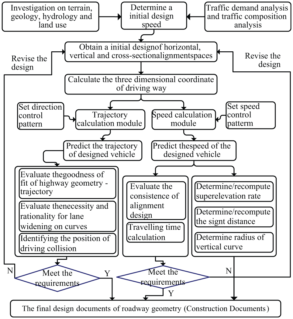
Alignment design procedure after the new design method proposed in this article is introduced.

Currently, some design institutes use a particular alignment optimization software when determining a route; after the design speed, control point, maximum tunnel length, highest pier height, and other constraints have been designated, the software searches for the “optimal” route for a highway.^25,26 By comparing the limits of the objective functions, a judgment can be made as to whether the route is “optimal.” The most commonly used objective functions include construction costs, maintenance costs, vehicle operation costs, environmental impact, and so on. Safety and comfort, being an important connotation of highway transportation, obviously should be one decision-making objective applied to route optimization. The use of the models in this article enables a designer to obtain trajectory collision positions, speed changes in adjacent alignment elements, longitudinal and lateral accelerations, and other parameters once the trajectory and speed have been predicted. Then, the level of safety and comfort of the alignment design can be precisely described. Therefore, the models can be added to existing alignment optimization software, and thus, the quality of travel along the designed highway can be enhanced. Furthermore, driving speed curves for the typical driving modes described in this article can provide calculation parameters for determining other evaluation indexes (optimization goals), such as fuel consumption, noise, exhaust, and travel time.

Examples of application of new method

The reconstruction of the Ganzi to Litang section of Provincial Road No. S217 in Sichuan Province, China was selected as the application of the new method. The original route followed the Yalong River, such that there are many sharp curves. This article takes sections Sta 100 + 580 to Sta 102 + 400 as examples. The design speed of road in reconstruction is 30 km/h. A cross section of a standard form, as provided by the design specification (JTG D20-2006), ²⁷ is adopted. A preliminary alignment design is obtained using the Hint software. Then, a procedure developed by the author is used to calculate the coordinates of the edge of the road every 5 m, after which the trajectory of three typical direction patterns is calculated. These are D1 (minimum length), D2 (minimum curvature), and D3 (mixed pattern of “keeping the vehicle in the middle of lane + minimum CCR”). Due to lighter traffic volume on the old road and in consideration of the driving habits observed, the pavement width available for drivers was set to 6.5 m for patterns D1 and D2, and to 4 m for D3. Then, the driving speed is determined based on the curvature of the trajectory. Accidents are more likely to occur during high-speed driving. Therefore, the minimum travel time is selected as the speed control mode and is set to S1. Finally, a check is made of the design consistency of the geometric features and their values are adjusted based on the trajectory and speed of the selected driving patterns.

It can be seen, in Figure 13(a), that the difference in the trajectory of the three patterns is significant. Among these, as presented in Figure 13(b), the trajectory curvature for pattern D1 is closest to that of the road centerline (designed curvature). The trajectory curvature of pattern D2 is significantly lower than the designed curvature except in the case of curves C7 and C8. Pattern D3 falls between the above two patterns. The lengths of C7 and C8 are obviously longer than the other 10 curves, so it can be assumed that the direction control behavior of various drivers will be more inclined to be convergence when the length of a curve is longer. The behaviors will diversify when the curves are shorter. Additionally, the trajectory curvature on the short straight between two adjacent curves is not zero in most cases. For example, when driving between C9 to C11 according to pattern D2, the driver steers the vehicle outward along the straight to decrease the trajectory curvature upon entering the curve. As a result, the trajectory of this tangent appears to be curved.

Figure 13.

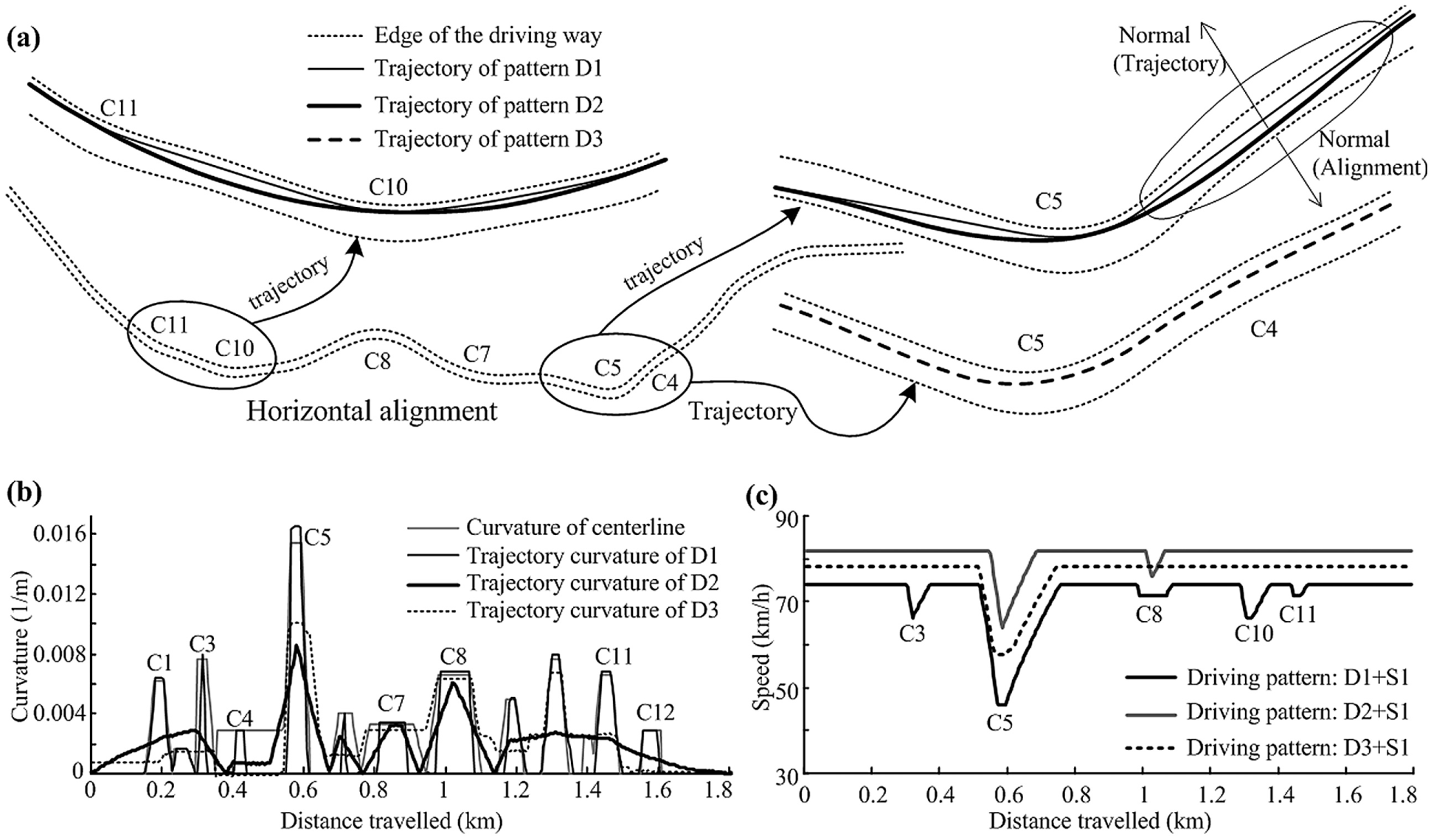
Trajectory–speed decision results and design improvement: (a) simulated trajectory of three driving patterns, (b) curvature of trajectory and curvature of road centerline, and (c) simulated speed of driving pattern: minimum traveling time.

Considering the goodness of fit between the trajectory and road geometry, there is a problem at C4: this curve deflects toward the left (in the travel direction C4 → C5), while the trajectory of pattern D2 at C4 deflects to the right. This will cause vehicles crossing the road edge easily. In addition, the lateral force due to super-elevation and centrifugal force are in the same direction, which results in the serious deterioration of the driving dynamics of the vehicles. The solution to this is to make a minor adjustment to the deflection angle of C5 and then to pull C4 into a straight line.

According to the speed profiles shown in Figure 13(c), the parameter for C5 also needs to be adjusted. Because a driver adopting patterns D1 and D3 need to slow down considerably upon driving into the curve, safety problems could occur if the driver were to be incapable of dealing with the change in speed. The values of the geometry features change and the trajectory and speed are re-simulated. The result gives rise to two means of controlling speed changes of less than 20 km/h. One is to widen the lane by 0.8 m on the inside of the curve and the other is to increase the curve radius from 65 to 78 m.

Conclusion

In this work, we proposed a new method of designing the horizontal alignment of a mountain highway, for which the basic premise involves predicting the trajectory of typical direction control patterns within the pavement width which can be used by drivers, and then predicting the speed for typical speed control patterns based on the curvature of the preview trajectory, and simultaneously using the trajectory and speed to determine the values for the geometric features of the designed road. A change in the radius, deflection angle, spiral, tangent length, and roadway width can all result in a change in the trajectory shape and speed amplitude. Therefore, these geometric features can then be controlled and regulated by the designer. Moreover, several typical driving patterns defined from human drivers give designer multiple options, the proposed method is therefore closer to the basic principles of road geometry design.

The new method is particularly suitable for the design of the horizontal alignment of medium and low-speed roads over rolling terrain, particularly the two-lane mountain roads. In consideration of the typical way in which road designers operate in some countries, the new method can be added to existing design procedures, constituting extra design steps. Simultaneously, the decision models can be appended to the existing route optimization software. The application of this new method in geometry design of Province Road No. S217 demonstrates its superiority compared with the current methods.

Given their higher ratio of engine power to vehicle mass, the speed of cars and light trucks is controlled by the horizontal alignment. In contrast, in addition to horizontal curves, the driving speeds of heavy trucks are very susceptible to the change in the grade. Therefore, in our future work, we will study the driving behavior of heavy trucks on mountain highways, in an attempt to establish a speed decision model that reflects the influences of driving habits, vehicle performance, loading factors, and road geometry. This will then be combined with the method described in this article to form a more comprehensive 3D alignment design method for mountain roads.