Sage Journals: Discover world-class research

Abstract

Dynamic penetration test by a penetrator is an important detection method for lunar exploration. The analysis of the dynamic penetration properties of the penetrator significantly helps to design the penetrator structure. In this article, the dynamic penetration mechanical model was established according to soil mechanics. Then, the discrete-element simulation model, which was established using the application program interfaces of the EDEM software, was used to simulate the penetration process. The penetration experiment demonstrated the accuracy of the dynamic penetration model and the discrete-element simulation model. This study of dynamic penetration model of a penetrator may provide technical support to the deep space exploration.

Keywords

Lunar exploration penetrator application program interfaces dynamics penetration model EDEM

Introduction

There are many mineral resources in the Moon, and the Moon is the nearest celestial body to the Earth. Moon explorations can improve the development of science and technology in a short period of time, help to harvest abundant resources, to develop greater knowledge about the origin of the cosmos, and to establish bases on the Moon in the future.

To acquire lunar soil samples, the main sampling methods consist of surface sampling and shallow depth sampling.^1,2 The main surface-sampling methods are digging sampling and hammering sampling; the main shallow-depth-sampling method is drilling. These methods have been performed by the United States and former Soviet Union in lunar exploration.^3,4

These sampling methods have the limitation of a high cost and low return. In addition, the soil samples cannot maintain their original state when these sampling methods are used. However, the penetration devices have smart structures, low power consumption, and light weight, so they can be used in challenging environments. Penetration devices have the advantages of low cost and high efficiency and have become a hotspot of study.

In 1996, the Space Research Centre of the Polish Academy of Sciences began the study of automatic penetrator used for the exploration of extraterrestrial objects, and the penetrator named MUPUS was designed to explore the comet.^5,6

During 2001 and 2003, the ESA and the DLR designed the penetrator used for Martian exploration based on the penetrator designed by Transmash. The outline dimension is φ27 mm × 280 mm, the mass is 890 g, the power is 3 W, and the penetration depth is 2 m. Besides, a sample collection device, which can collect soil for 0.2 cm³, was on the front part of the penetrator.^7–9

Then, from 2003 to 2006, according to the Martian penetration exploration mission, Italian Galileo Avionica asked the DLR to research the penetrator again. And the DLR designed the IMS penetrator based on the PLUTO penetrator, which had smaller volume and less power. The outline dimension is Φ26 mm × 251 mm, the mass is 435 g, the power is 1.3 W, and the theoretical penetration depth is 3 m. Penetration speed is 0.6 m/h and the practical penetration depth is 1.25 m.¹⁰

During 2006 and 2008, in order to carry out the penetration exploration, the SRC PAS designed the KPET penetrator based on the MUPUS penetrator.^11,12

In 2008, the NASA designed the MMUM penetrator for the Martian or the lunar dynamic penetration test based on the PLUTO penetrator. The outline dimension is Φ40 mm × 600 mm, the mass is 200 g, the power is 10 W, and the theoretical penetration depth is 2 m.¹³

In 2013, the State Key Laboratory of Robotics and System of the Harbin Institute of Technology (HIT) designed a kind of penetrator whose outline dimension is φ35 mm × 325 mm, the mass is 420 g, the power is 10 W, and the penetration depth is 1 m.¹⁴

Although there have been some achievements using the penetration devices, theoretical studies regarding the use of the penetration device are lacking. No successful cases detected the planet using penetration devices. The analysis of the dynamic penetration properties of the penetrator has a significant value to help design the penetrator structure. In this article, based on the results from a previous study on two arc-shaped front noses of penetrator,^15–17 the axial resistance of the penetrator with concave arc-shaped nose is smaller than the convex one. Therefore, it is necessary to study the dynamic process of the concave arc-shaped nose of the penetrator. The dynamic penetration mechanical model was established according to soil mechanics. Then, the discrete-element simulation model, which was established using the application program interfaces (APIs), was used to simulate the penetration process. The penetration experiment demonstrated the accuracy of the theory. This study may provide technical support to the penetration programs of the deep space exploration.

Mechanical model of the penetrator in the penetration process

A concave arc-shaped front nose

Because the front nose first contacts the soil, the shape and the structural parameters of the front nose have a significant influence on the penetration feature of the penetrator. To maintain a depth of penetration above 1 m, a proper shape of the front nose should be determined.

The concave arc-shaped front nose is shown in Figure 1. The penetrator is considered as a rigid body in the penetration process, which remains in its original shape in the penetration process.

Figure 1.

Structural model of the concave arc-shaped front nose.

In Figure 1, R is the radius of the penetrator shell, S is the radius of the curvature of the camber, l is the length of the concave arc-shaped front nose; β is the angle between any point of the camber and the vertical direction; and β₀ is the angle between the peak of the camber and the vertical direction.

The caliber-radius-head is defined according to the following equation

ψ = \frac{S}{2 R}

(1)

Model of soil failure

In the penetration process of the penetrator, the region of soil failure is shown in Figure 2. According to Figure 2, during the penetration process, the soil near concave arc-shaped front nose of penetrator consists of the compacted region I, the transition region II, and the passive region III. The soil in region I moves down with the penetrator in the penetration process. The soil in region II initially moves to region III, and the soil in region III will fail when the pressure improves to a certain extent. There are two slip lines in region II, and the equation of the slip is expressed as

r = r_{0} e^{θ tg φ}

(2)

where $φ$ is the internal friction angle of lunar soil; $θ$ is the polar angle in the polar coordinates (point B is the polar point and BE is the polar axis); and r₀ is the length of BE.

Figure 2.

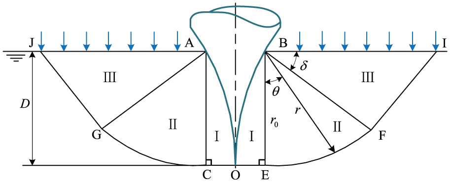
Region of soil failure.

The mechanic state of block BFHK is shown in Figure 3 when the soil in region III begins to fail.

Figure 3.

Mechanic state of the block BEFK.

In Figure 3, q is the soil stress on plane BK; q = γh, where γ is the bulk density of the soil.

h = {\begin{matrix} r_{0} N_{φ} / 3 & D < l \\ D - l + r_{0} N_{φ} / 3 & D > l \end{matrix}

N_{φ} = 1 + \frac{e^{(π / 2 + φ) tg φ} \cdot \sin^{2} (π / 4 - φ / 2)}{1 + e^{(π / 4 + φ) tg φ} \cdot \sin (π / 4 - φ / 2)}

where D is the penetration depth of the penetrator; l is the length of the concave arc-shaped front nose; p_P is the normal Rankine’s passive earth pressure on the surface of FK; C is the cohesion of soil; p_n is the normal stress on surface EF; p_ntgφ is the friction force on surface EF; p_r is the joint stress of p_n and p_ntgφ; φ is the angle between p_r and p_n; p_F is the Rankine’s active earth pressure on the surface of BE; δ is the angle between the slip line and the horizontal plane, δ = π/4 −φ/2; and r₀ is the length of BE.

From the geometric relationships in Figure 4, we easily see that

{\begin{matrix} \bar{BF} = r_{0} e^{(π / 4 + φ / 2) \tan φ} \\ \bar{BK} = \bar{BF} \cos δ = r_{0} e^{(π / 4 + φ / 2) \tan φ} \cos (π / 4 - φ / 2) \\ \bar{FK} = \bar{BF} \sin δ = r_{0} e^{(π / 4 + φ / 2) \tan φ} \sin (π / 4 - φ / 2) \end{matrix}}

(3)

Figure 4.

Mechanic state of the block BOE.

Based on the Mohr–Coulomb failure criteria, the normal Rankine’s passive earth pressure on the surface FK is expressed by the following equation

p_{P} = q \cot^{2} (π / 4 - φ / 2) + 2 c \cot (π / 4 - φ / 2)

(4)

The surface BE can be considered to be the retaining wall because of the fact that the soil in region I moves down with the penetrator. Taking point B as the centroid, we can get the following equation according to the static equilibrium condition of block BEFK

\sum M_{B} = M_{p_{F}} - M_{p_{P}} - M_{q} - M_{c} = 0

(5)

And we can easily get that

{\begin{matrix} M_{p_{F}} = \frac{1}{2} p_{F} {(\bar{BF})}^{2} = \frac{1}{2} p_{F} {(r_{0})}^{2} \\ M_{p_{P}} = \frac{1}{2} p_{P} {(\bar{HK})}^{2} = \frac{1}{2} {(r_{0})}^{2} e^{(π / 2 + φ) \tan φ} [γ H \cos^{2} (π / 4 - φ / 2) + c \cos φ] \\ M_{q} = \frac{1}{2} q {(\bar{BK})}^{2} = \frac{1}{2} γ H {(r_{0})}^{2} e^{(π / 2 + φ) \tan φ} \cos^{2} (π / 4 - φ / 2) \\ M_{c} = \int c d s \cos φ r = \int_{0}^{(π / 4 + φ / 2)} c \frac{r d θ}{\cos φ} \cos φ r = \frac{1}{2} c {(r_{0})}^{2} \cot φ [e^{(π / 2 + φ) \tan φ} - 1] \end{matrix}

(6)

Substituting equation (6) into equation (5), we find that the Rankine’s active earth pressure on the surface BE is as follows

p_{F} = q N_{q} + c N_{c}

(7)

where

N_{q} = 2 e^{(π / 2 + φ) \tan φ} \cos^{2} (π / 4 - φ / 2)

N_{c} = (\cos φ + \cot φ) e^{(π / 2 + φ) \tan φ} - \cot φ

here, N_q and N_c are the bearing capacity coefficients of the soil.

The mechanical state of the block BOE in the compacted region is to be analyzed after we get the Rankine’s active earth pressure on the surface BE p_F. Its mechanical state is shown in Figure 4.

In Figure 4, τ_F is the friction stress on the surface BE, τ_F = c + p_Ftgφ; P₀ is the normal stress on the surface OE; τ₀ is the friction stress on the surface OE, τ₀ = c + p₀tgφ; p is the normal stress on the surface OB; and f is the friction stress on the surface OB.

The force between the concave arc-shaped front nose of the penetrator and the block BOE is expressed by the following equation

{\begin{matrix} Q_{x} = \int (p \sin θ - f \cos θ) d s \\ Q_{y} = \int (p \cos θ + f \sin θ) d s \end{matrix}

(8)

According to the static equilibrium condition of block BOE, we find

{\begin{matrix} Q_{x} - p_{F} \bar{BE} - τ_{0} \bar{OE} = 0 \\ p_{0} \bar{OE} + τ_{F} \bar{BE} - Q_{y} = 0 \end{matrix}

(9)

Substituting equations (7) and (8) into equation (9), we obtain the following radial stress

p = (\begin{matrix} \begin{array}{l} \frac{2 ψ γ R N_{φ} N_{q} (1 - {tg}^{2} φ) \cos^{2} β}{3 [(μ tg φ - 1) \sin β + (μ + tg φ) (1 - \cos β)]} \\ + c \frac{N_{c} (1 - {tg}^{2} φ) \cos β - tg φ \cos β - \sin β + 1}{(μ tg φ - 1) \sin β + (μ + tg φ) (1 - \cos β)} \end{array} & D < l \\ \begin{array}{l} \frac{2 ψ γ R N_{q} (\frac{D}{2 ψ R} - \cos β_{0}) \cos β_{0} (1 - {tg}^{2} φ)}{(μ tg φ - 1) \sin β_{0} + (μ + tg φ) (1 - \cos β_{0})} \\ + c \frac{N_{c} (1 - {tg}^{2} φ) \cos β - tg φ \cos β - \sin β + 1}{(μ tg φ - 1) \sin β + (μ + tg φ) (1 - \cos β)} \end{array} & D \geq l \end{matrix})

(10)

According to the above analysis, the normal stress on the surface OB in the penetration is obtained. We can use its value to help analyze and calculate the axial resistance of the penetrator.

Axial resistance model of the penetrator

Assume that the penetrator will always travel along the vertical direction during penetration. The penetration process can be divided into three stages before the penetrator completely penetrates into the soil.

1. D < l: in this stage, resistance of the penetrator focuses on concave arc-shaped front nose, and the mechanical analysis is shown is Figure 5.

Figure 5.

Mechanical analysis of the concave arc-shaped nose.

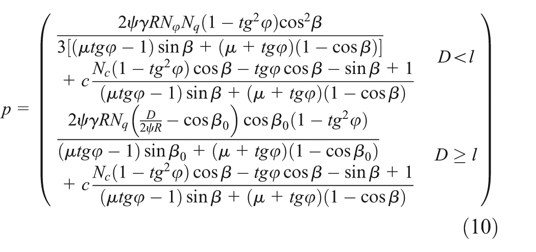
According to Figure 5, the infinitesimal axial resistance of the penetrator is expressed by the following equation

\begin{array}{l} d F = 2 π x (p \cos θ + f \sin θ) d s \\ = 4 π ψ R (1 - \sin θ) (p \cos θ + f \sin θ) d s \end{array}

(11)

Then, the total axial resistance is derived after the integral operation of equation (11)

F = \int d F = \int_{\frac{π}{2}}^{β} 2 π x (p \cos θ + f \sin θ) 2 ψ R d θ = K_{1} ψ^{3} + K_{2} ψ^{2}

(12)

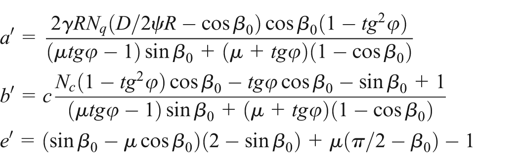
where

\begin{matrix} K_{1} = 4 π R^{2} ae \\ K_{2} = 4 π R^{2} be \end{matrix}

\begin{array}{l} a = \frac{2 γ R N_{φ} N_{q} (1 - {tg}^{2} φ) \cos^{2} β}{3 [(μ tg φ - 1) \sin β + (μ + tg φ) (1 - \cos β)]} \\ b = c \frac{N_{c} (1 - {tg}^{2} φ) \cos β - tg φ \cos β - \sin β + 1}{(μ tg φ - 1) \sin β + (μ + tg φ) (1 - \cos β)} \\ e = (\sin β - μ \cos β) (2 - \sin β) + μ (π / 2 - β) - 1 \end{array}

2. l < D < (L + l): L is the noumenon length of the penetrator. In this state, the concave arc-shaped front nose of the penetrator has completely penetrated into the soil. The total axial resistance can be obtained by substituting β = β₀ into equation (15). Besides, in this state, the soil also contacts the lateral surface of the penetrator. The mechanical model of the lateral surface is shown in Figure 6.

Figure 6.

Mechanical model of the lateral surface.

The equation of the total axial resistance on the concave arc-shaped front nose in this state is like equation (12), and it is as follows

F' = K_{1'} ψ^{3} + K_{2'} ψ

(13)

where

\begin{matrix} K_{1'} = 4 π R^{2} a' e' \\ K_{2'} = 4 π R^{2} b' e' \end{matrix}

\begin{array}{l} a^{'} = \frac{2 γ R N_{q} (D / 2 ψ R - \cos β_{0}) \cos β_{0} (1 - {tg}^{2} φ)}{(μ tg φ - 1) \sin β_{0} + (μ + tg φ) (1 - \cos β_{0})} \\ b^{'} = c \frac{N_{c} (1 - {tg}^{2} φ) \cos β_{0} - tg φ \cos β_{0} - \sin β_{0} + 1}{(μ tg φ - 1) \sin β_{0} + (μ + tg φ) (1 - \cos β_{0})} \\ e^{'} = (\sin β_{0} - μ \cos β_{0}) (2 - \sin β_{0}) + μ (π / 2 - β_{0}) - 1 \end{array}

Besides, the lateral surface is considered as the retaining wall, and then the passive earth pressure is expressed by the following equation according to Rankine’s earth pressure theory

p_{P} = γ (D - y) K_{P} + 2 c \sqrt{K_{P}}

(14)

where K_P is the coefficient of the passive earth pressure, and $K_{P} = t g^{2} (45 ° + φ / 2)$ .

So, the horizontal positive pressure on the infinitesimal surface is

d N = p_{P} dA = 2 π p_{P} R dy

(15)

The friction force between the soil and the lateral surface is

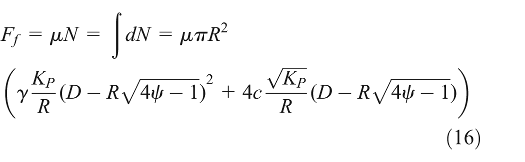
\begin{array}{l} F_{f} = μ N = \int d N = μ π R^{2} \\ (γ \frac{K_{P}}{R} {(D - R \sqrt{4 ψ - 1})}^{2} + 4 c \frac{\sqrt{K_{P}}}{R} (D - R \sqrt{4 ψ - 1})) \end{array}

(16)

So, the axial resistance force of the penetrator is expressed by the following equation

F = F' + F_{f}

(17)

3. D ≥ (L + l): in this state, the axial mechanical analysis of the penetrator is shown in Figure 7.

Figure 7.

Axial mechanical analysis of the penetrator.

In this state, the total axial force of the concave arc-shaped front nose F″ is

F ″ = F'

(18)

The friction force between the soil and the lateral surface is given by

\begin{array}{l} F_{f}' = 2 μ L \sqrt{K_{P}} (π R γ \sqrt{K_{P}} (2 D - L) + c) \\ - 4 π R^{2} μ γ K_{P} L \sqrt{4 ψ - 1} \end{array}

(19)

So, the axial force that resists the motion of the penetrator can be obtained as follows

F = F ″ + F_{f}'

(20)

According to the above analysis, the axial resistance model of the penetrator in the penetration is obtained. And then, we can use its value to establish the dynamical model of the penetrator in the penetration process.

Dynamic model in the penetration process

After the impact hammer impacts the cone, they will move down together. In addition, the concave arc shape of the penetrator will rapidly penetrate into the soil. Then, the downward movement speed will descend with the increase in penetration depth; so, the study of penetration dynamics focuses on the second and third states of penetration.

When the impact hammer and cone move down together, the following equation is obtained according to Newton’s Second Law of Motion

M \frac{d v}{d t} = M \frac{d v}{d D} \frac{d D}{d t} = Mv \frac{d v}{d D} = F

(21)

where M is the total mass of the impact hammer and cone (kg) and v is the downward motion speed (mm/s).

The impact hammer and the cone move down at an identical initial speed V after they impact at any time, and every penetration process finishes when their speed is zero. In this article, we assume that the penetration depth D_N₋₁ increases to D_N after the Nth penetration.

The following equation is obtained by integrating equation (21)

\int_{V}^{0} Mv d v = \int_{D_{N - 1}}^{D_{N}} F d D

(22)

In the second penetration state of the penetrator, l < D < l + L; we substitute equation (17) into equation (22); then, D_N and D_N₋₁ are expressed as follows

D_{N} = A_{2} + \frac{K_{2}}{A_{2}} + R \sqrt{4 ψ - 1} - \frac{2 c}{γ \sqrt{K_{P}}}

(23)

where

\begin{matrix} A_{2} = {(\sqrt{{(B_{2} + E_{2} - G_{2})}^{2} - K_{2}^{3}} + B_{2} + E_{2} - G_{2})}^{\frac{1}{3}} \\ B_{2} = \frac{3 (M V^{2} + 2 D_{N - 1} F_{2}')}{4 π R γ μ K_{P}} + \frac{D_{N - 1}}{2} D_{N - 1}^{2} \\ - \frac{3 R D_{N - 1}}{2} \sqrt{4 ψ - 1} (D_{N - 1} - R \sqrt{4 ψ - 1}) \\ E_{2} = (\frac{3 c}{γ \sqrt{K_{P}}} - \frac{3 R \sqrt{4 ψ - 1}}{2}) \\ \times (\frac{F_{2}'}{π R γ μ K_{P}} - \frac{4 cR}{γ \sqrt{K_{P}}} \sqrt{4 ψ - 1} + R^{2} (4 ψ - 1)) \\ G_{2} = {(\frac{2 c}{γ \sqrt{K_{P}}} - R \sqrt{4 ψ - 1})}^{3} \\ K_{2} = \frac{4 c^{2}}{γ^{2} K_{P}} - \frac{F_{2}'}{π R γ μ K_{P}} \end{matrix}

Assuming that the initial state in the second penetration state of the penetrator is that the concave arc-shaped front nose is correctly buried by the soil, the initial depth is $D_{0} = R \sqrt{4 ψ - 1}$ . Substituting D₀ into equation (23), we find

D_{1} = A_{2_{0}} - F_{2}' / (g A_{2_{0}}) + R \sqrt{4 ψ - 1}

(24)

where

\begin{matrix} A_{2_{0}} = {(\sqrt{(\frac{F'_{2}^{3}}{g^{3}} + \frac{9 M^{2} V^{4}}{16 g^{2}})} + \frac{3 M V^{2}}{4 g})}^{\frac{1}{3}} \\ g = π R γ μ K_{P} \end{matrix}

In the third penetration state of the penetrator, D > l + L. Substituting equation (20) into equation (23), D_N and D_N₋₁ can be expressed as follows

D_{N} = D_{N - 1} + A_{3} + \sqrt{M V^{2} / B_{3} + A_{3}^{2}}

(25)

where

\begin{array}{l} B_{3} = \frac{4 π R γ [R N_{q} (1 - {tg}^{2} φ) ψ^{2} \cos β_{0} e_{2^{'}} + μ L K_{P}]}{(μ tg φ - 1) \sin β_{0} + (μ + tg φ) (1 - \cos β_{0})} \\ A_{3} = R \sqrt{4 ψ - 1} - D_{N - 1} + \frac{2 π R γ μ K_{P} L^{2}}{B_{3}} \end{array}

D_{1} = R \sqrt{4 ψ - 1} + L + A_{3_{0}} + \sqrt{M V^{2} / B_{3} + A_{3_{0}}^{2}}

(26)

where $A_{3_{0}} = 2 π R γ μ K_{P} L^{2} / B_{3} - L$ .

Theoretical penetration depth according to the penetration dynamics

According to the established theoretical equation, the program chart to calculate the penetration depth is shown in Figure 8.

Figure 8.

Program chart to calculate the penetration depth.

In this article, the impact work in every impact state is set to be W = MV²/2 = 1 J, and the penetration depths of the penetrator with different structural parameters can be obtained by changing the structural parameter ψ. Figure 9 shows the change in penetration depth with the number of impact times.

Figure 9.

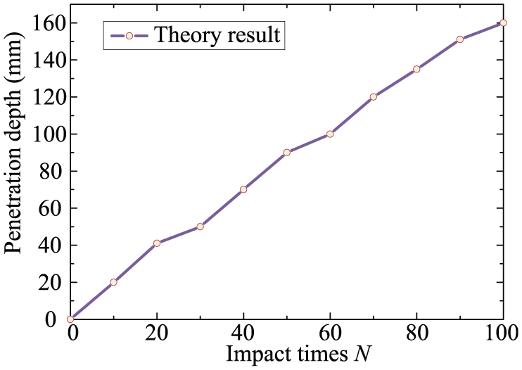
Change in penetration depth with the impact times.

According to Figure 9, in the simulation process, the penetration depth increases with the increase in the number of impact times. The penetration depth of the cone is 160 mm when the number of impact times is 100.

Discrete-element simulation model

To demonstrate the accuracy of the provided theory, the discrete-element simulation model was established to simulate the interaction process between the soil and the penetrator.

Discrete-element simulation model of the lunar soil

Lunar soil is composed of numerous micro particles, and the shapes of the particles are complicated and fickle. In the simulation process, the irregular lunar soil particles are alternated by spherical particles after the stacking angle test. In this article, to decrease the simulation time based on the simulation accuracy, the discrete-element simulation model of the soil has three types of particles with different diameters: 0.5, 1, and 1.5 mm. The simulation model of the lunar soil is shown in Figure 10.

Figure 10.

Discrete-element simulation model of the lunar soil.

The physical and mechanical properties of the lunar soil in the discrete-element simulation model are determined by parameter matching. The concrete method is as follows: first, the mechanical properties of the soil are determined by three-triaxial compression experiment, and then, the parameters of the discrete-element simulation model are changed until the results of the three-triaxial compression simulation in the EDEM software are similar to the result of the three-triaxial compression experiment. According to this parameter matching method, the final material parameters and contact parameters of the soil and the penetrator are shown in Tables 1 and 2, respectively.

Table 1.

Material parameters.

Material parameters	Lunar soil	Penetrator	Unit
Density	1750	1750	kg/m³
Poisson’s ratio	0.3	0.3	−
Shear modulus	2 × 10⁷	2 × 10¹⁰	Pa

Table 2.

Contact parameters.

Contact parameters	Lunar soil–lunar soil	Lunar soil–penetrator	Unit
Coefficient of restitution	0.1	0.2	−
Coefficient of static friction	0.574	0.3	−
Coefficient of rolling friction	0.01	0.01	−

Discrete-element simulation model of the interaction process between the lunar soil and the penetrator

Because of the motion limitation of the geometry in the EDEM software, the traditional simulation model cannot simulate the dynamic penetration process of the penetrator. Thus, we wrote simulation programs and imbedded them into the EDEM software through the APIs of EDEM. The simulation program flow chart is shown in Figure 11.

Figure 11.

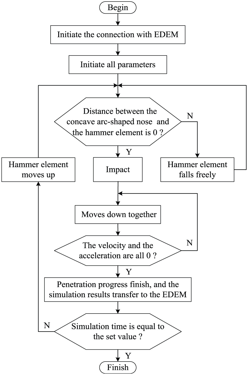
Simulation program flow chart.

In the simulation, the impact work of every time is 1 J. The dynamic interaction process between the concave arc-shaped nose and the lunar soil in one time of the penetration as shown in Figure 12.

Figure 12.

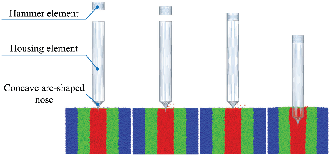
Dynamic penetration process in one time.

Figure 13 shows the soil failure condition when the number of impact times between the hammer element and the concave arc-shaped nose is 100.

Figure 13.

Soil failure condition.

With the increase in number of impact times, the failure of the lunar soil becomes increasingly more serious according to Figure 13. In addition, the red and blue lunar soil particles mix together, particularly in the area of the concave arc-shaped nose. Figure 14 shows the change in penetration depth with the number of impact times when the structural parameter ψ is 2.

Figure 14.

Change in penetration depth with the number of impact times.

According to Figure 14, in the simulation process, the penetration depth first rapidly increases with the increase in the number of impact times, but the increase in the penetration depth with the increase in the number of impact times subsequently becomes slow. The penetration depth of the cone is 102 mm when the number of impact times is 100.

Dynamical penetration experiment

Except for the penetration simulation, we also carried out the penetration experiment to prove the accuracy of our theory. The experiment and facilities are as follows.

Experiment table

To perform the penetration experiment, the experiment facilities were produced as shown in Figure 15. The penetration experiment table consists of the drive rod, guide rod, impact plate A, impact plate B, sleeve, and trestle table. The parameters of the experiment facilities are shown in Table 3.

Figure 15.

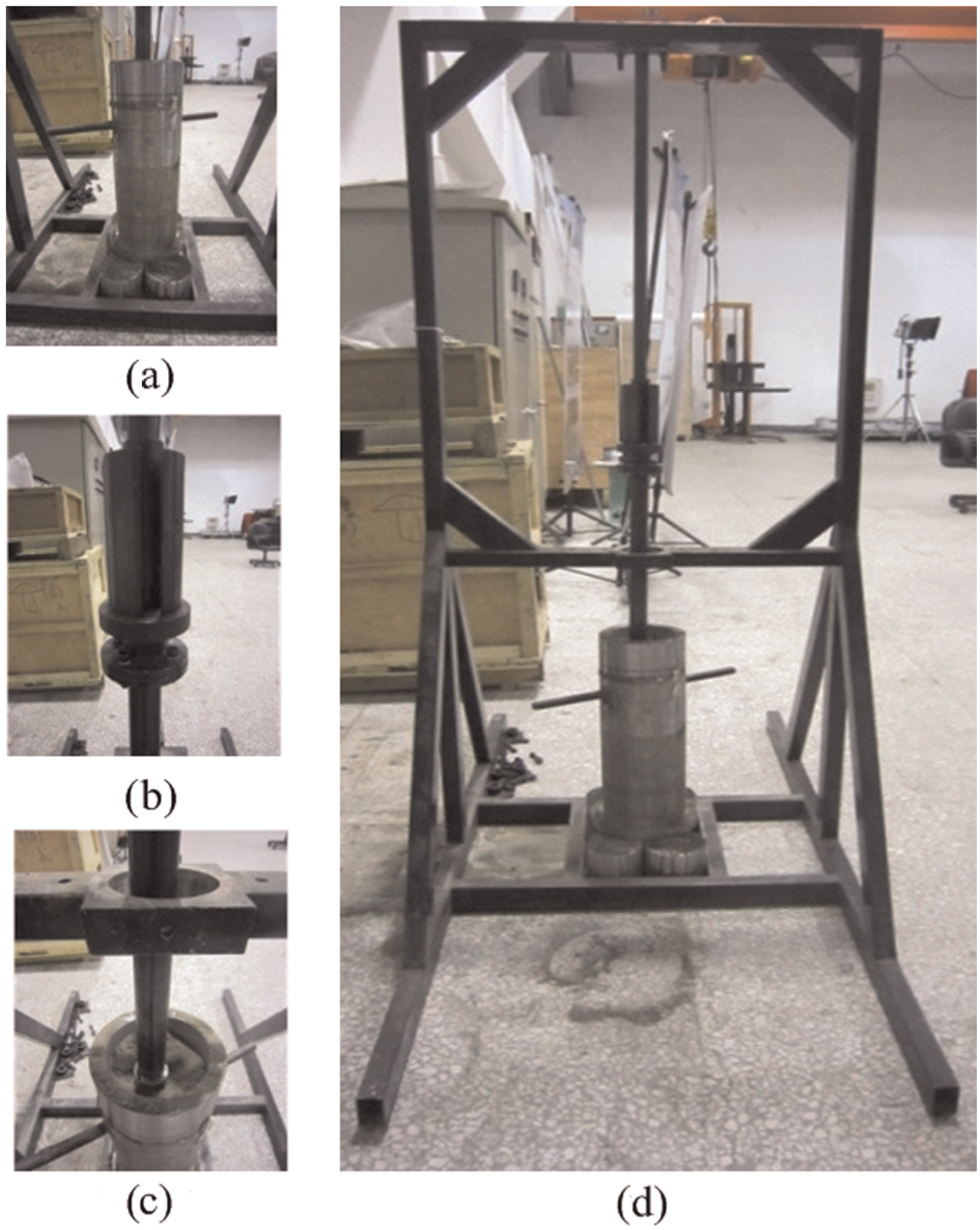
Penetration experiment facilities: (a) lunar soil container, (b) hammer element, (c) housing element, and (d) impact test device.

Table 3.

Parameters of the penetration experiment.

Parameters	Value	Unit
Whole size of the impact test device	1.35 × 0.65 × 1.6	m
Mass of hammer element	950	g
Mass of weight	180/210/250	g
Length of housing element	356	mm

Penetration experiment

When we performed the penetration experiment, the experiment parameters were set according to Table 4, and the penetration experiment is shown in Figure 16. The experiment result is shown in Figure 17.

Table 4.

Experiment parameters.

Parameters	Value	Unit
Impact energy	1.2	J
Total mass of hammer element	1200	g
Diameter of the lunar soil container	150	mm
Height of lunar soil container	500	mm

Figure 16.

Penetration experiment and the concave arc-shaped nose.

Figure 17.

Change in penetration depth with the impact times.

According to Figure 17, in the simulate regolith, the penetration depth is approximately 90 mm when the number of impact times is 100.

To demonstrate the accuracy of our impact dynamic theory, the theoretical, simulation, and experiment results are listed in Figure 18.

Figure 18.

Different results.

According to Figure 18, the simulation result curve is notably close to the experiment result curve, which demonstrates the accuracy of the discrete-element simulation model. Because of some of the simplified treatments and many empirical parameters provided by soil mechanics, there are some errors between the theory result and the other results, but the entire variation trend of the theory result curve is close to the others. The established dynamic penetration model in this article can be used to analyze the dynamic penetration properties of the penetrator. The parameters provided by the soil mechanics will be calibrated to improve the accuracy trend of the theory result.

Conclusion and outlook

In this article, the dynamic penetration model of the penetrator was established. To demonstrate the accuracy of the theoretical model, the discrete-element simulation model was established to simulate the penetration process. Finally, the penetration experiment was also performed. The theoretical, simulation, and experiment results show a good agreement, and the study method proposed in this article might be a kind of method that can be used for planetary penetration exploration. In the future, the parameters given by soil mechanics will be calibrated to improve the accuracy trend of the theory result.

Footnotes

Academic Editor: ZW Zhong

Declaration of conflicting interests

The author(s) declared no potential conflicts of interest with respect to the research, authorship, and/or publication of this article.

Funding

The author(s) disclosed receipt of the following financial support for the research, authorship, and/or publication of this article: This project was supported by the National Nature Science Foundation of China (nos 51575123 and 51575122), Self-Planned Task of State Key Laboratory of Robotics and System, Harbin Institute of Technology (HIT; no. SKLRS201616B), the Fundamental Research Funds for the Central Universities (HIT.NSRIF.2017028), and the International Science and Technology Cooperation Program of China (no. 2014DFR50250).

References

Ouyang

ZY.

Scientific objectives of Chinese lunar exploration project and development strategy. Adv Earth Sci 2004; 19: 351–358.

Deng

Ouyang

Wang

. Physical and mechanical properties of lunar regolith. J Mineral Petrol 2004; 24: 14–19.

Davies

Phipps

Taylor

. UK lunar science missions: Moonlite & Moonraker. In: Proceedings of the 3rd international conference on recent advances in space technologies, Bremen, Germany, 14–16 June 2007, pp.774–779. USA: IEEE.

Jiang

Piao

Zhang

. Typical cases analysis and prospects for extraterrestrial subsurface boring exploration. J Deep Space Explor 2016; 3: 68–76.

Grygorczuk

Banaszkiewicz

Seweryn

. MUPUS Insertion device for the Rosetta mission. J Telecommun Inf Tech 2007; 1: 50–53.

Seweryn

Skocki

Banaszkiewicz

. Determining the geotechnical properties of planetary regolith using Low Velocity Penetrometers. Planet Space Sci 2014; 99: 70–83.

Richter

Coste

Gromov

. Development and testing of subsurface sampling devices for the Beagle 2 lander. Planet Space Sci 2002; 50: 909–913.

Wright

Sims

Pillinger

CT.

Scientific objectives of the Beagle 2 lander. Acta Astronaut 2003; 52: 219–225.

Alex

Andrew

Charles

. Vanguard—a European robotic astrobiology-focussed Mars sub-surface mission proposal. Acta Astronaut 2005; 56: 397–407.

10.

Jerzy

Łukasz

Bartosz

. Hammering mechanism for HP3 experiment (InSight). In: Proceedings of the 43rd aerospace mechanisms symposium, Santa Clara, CA, 4–6 May 2016, pp.415–428. USA: AMS Program.

11.

Banaszkiewicz

Seweryn

Wawrzaszek

A sensor to perform in situ thermal conductivity determination of cometary and asteroid material. Adv Space Res 2007; 40: 226–237.

12.

Tulej

Iakovleva

Leya

. A miniature mass analyser for in situ elemental analysis of planetary material–performance study. Anal Bioanal Chem 2011; 399: 2185–2200.

13.

Bualat

Kobayashi

Lee

. Flexible rover architecture for science instrument integration and testing. In: Space 2006 Conference, San Jose, USA, 19–21 September 2006, pp.2089–2098. USA.

14.

Shen

Jiang

. Study on optimization of structure parameters to the penetrator. In: IEEE international conference on mechatronics and automation, Harbin, China, 7–10 August 2016, pp.1518–1523. USA: IEEE.

15.

Shen

Hou

Jiang

. On two arc-shaped sensor front noses for smaller axial resistance of mole. Sens Lett 2015; 13: 161–164.

16.

Shen

Hou

Qin

. Shape of mole nose providing minimum axial resistance. Robot Biomi 2014; 1: 1–10.

17.

Qin

Hou

Quan

. An arc-shaped front nose for the mole in space exploration. In: IEEE international conference on robotics and biomimetics, Shenzhen, China, 12–14 December 2013, pp.56–61. USA: IEEE.

Study on the dynamic characteristics of a hammer-driven-type penetrators in the penetration process

Abstract

Keywords

Introduction

Mechanical model of the penetrator in the penetration process

A concave arc-shaped front nose

Model of soil failure

Axial resistance model of the penetrator

Dynamic model in the penetration process

Theoretical penetration depth according to the penetration dynamics

Discrete-element simulation model

Discrete-element simulation model of the lunar soil

Discrete-element simulation model of the interaction process between the lunar soil and the penetrator

Dynamical penetration experiment

Experiment table

Penetration experiment

Conclusion and outlook

Footnotes

Declaration of conflicting interests

Funding

References