Sage Journals: Discover world-class research

Abstract

Because the coal-bed methane field is influenced by factors such as low pressure, slow velocity, terrain, and condensed water, which lead to the fact that the design is different from gathering design of conventional gas field, how to make full use of wellhead pressure and maximize the wellhead pressure ability is an important link of surface engineering optimization. Therefore, we need to analyze the factors which influence the pressure drop of the gas-gathering pipe network to improve the efficiency of the coal-bed methane field surface gathering. We first contrasted the two hydraulic analysis software (PIPEPHASE and TGNET) for the analysis of coal seam gas field adaptability. By comparing the simulation results with the actual data, we found that the PIPEPHASE software is better to analyze the hydraulic situation of pipe network in the coal-bed methane field. Then, using PIPEPHASE for network simulation and contrasting the 9 state equations and 26 kinds of pressure drop formula calculation results, SRK state equation and BBM pressure drop formula are recommended. We analyze the inlet temperature, pressure, and other nine factors affecting gas extraction pipeline pressure drop according to the practical experience and put forward the suggestions as follows: (1) in order to reduce the pressure drop and increase the ability of pipeline, burying pipeline under the permafrost and improving the inlet pressure are suggested; (2) The higher the inlet pressure, the more obvious the pipeline efficiency influences the pipeline pressure drop, so the inlet pressure and pipeline efficiency should be reasonably controlled in order to reduce the pressure drop; (3) The higher the pipeline pressure, the greater the wall roughness influences the pipeline pressure drop, also the greater the pressure can damage, so we should try to use small wall roughness materials.

Keywords

Coal-bed methane field gas-gathering pipe network pressure drop TGNET PIPEPHASE hydraulic adaptability

Introduction

Weymouth empirical formula is proposed by American Weymouth in 1912; this is a pure empirical formula in the initial stage of natural gas pipeline, which is characterized by small diameter, low volume, poor natural gas purification, pipe technology, poor installation process, pipe wall surface roughness, formula pipe wall roughness of the larger selection (κ = 0.0508 mm, which is a constant), and air flow in the square area of resistance work. Weymouth formula is not only better in accordance with the actual situation at the time but also simple; so for decades, many countries have adopted this formula. At present, the progress of the pipe technology has made the surface roughness of the steel pipe to improve greatly during the period the empirical formula was proposed by Weymouth; the gas–liquid separation effect of the gas-gathering station and the pigging and corrosion control technology of the natural gas transportation process have been improved which makes the flow calculation of the Weymouth formula often lower than the actual value; so, many countries no longer use Weymouth formula.^1–5

In 1936, Hardy Cross proposed the Hardy Cross method to solve the nonlinear equations in the pipe network. With the development of the computer technology, in the 1950s, the method was applied to the computer solution of water supply hydraulic pipe network in the hydraulic calculation and quickly extended to the heating pipe network and gas pipe network in the hydraulic calculation. So far, the computer technology is widely used in the gas pipeline network hydraulic calculation and rapid development. Subsequently, DM Martin and Peters⁶ applied the Newton–Raphson method to the equations of the solution loop and the solution of the nodal points and improved the iteration speed. AG Collioas and Johnson⁷ used the finite element method to solve the nodal equations. DJ Wood and Charles⁸ and others introduced the linearization theory, used to solve the pipe equations. These theories provide a solid foundation for later researchers to study the hydraulic calculation of steady-state gas networks.⁹

Twentieth century computer technology has made amazing development, resulting in a large number of auxiliary management software; hydraulic simulation software also came into being. The earliest development is the British ESI company; their software Pipeline Studio for Gas TGNET is widely recognized.¹⁰ The software is capable of transient and steady-state simulations of single-phase flow in a gas line. It can be used to evaluate and guide the design and operation of natural gas pipelines, so that the system performance can be optimized. The software can be used to build the model and view the results of steady-state simulation. More conveniently, US STONER company developed simulation software SWS and SPS. The former is used for simulation and design of gas steady-state pipeline network, and the latter is used for dynamic simulation and simulation of long-distance pipeline. In addition, there are ACROLOLE software developed by French Gas Company, PCASIM pipeline simulation software developed by Novacorp Corporation of Canada, and Dispatching Tutoral System (DTS) developed by Snamprogetti Company of Italy.^11,12 In addition, SUNRISE SYSTEMS LIMITED, LIWACOM of Germany, Kongsberg of Norway, SPT, and so on, have also developed their own simulation software to improve the simulation accuracy.

Basic theory

Due to the need to compare the adaptability of TGNET software and PIPEPHASE software, we need to analyze the equations which need to be used in the two kinds of software.

Equations in TGNET software

TGNET is natural gas transmission and distribution system calculation software developed by ESI Company. TGNET can simulate not only a simple one-pipe delivery model but also multiple complex recycle networks which have multiple sources and users, compressors and coolers, and other equipments. The software provides four state equations including “SAREM,”“BWRS,”“PENG,” and “SRK.” Five pressure drop formulas are also included in the TGNET such as “AGA,”“Colebrook,”“Pan (A),” and “Pan (B).”^13–19

State equations

TGNET software mainly has Sarem state equation, Peng–Robinson equation, and BWRS equation.

Sarem state equation

Z = \sum_{m = 0}^{5} \sum_{m = 0}^{5} A_{mm} P_{m} (\frac{2 P_{r} - 15}{14.8}) P_{n} (\frac{2 T - 4}{1.9})

(1)

Sarem state equation has a high accuracy in the normal operating pressure range of most natural gas systems. It requires less description of the gas parameters, and it only needs the relative density, calorific value, and CO₂ content. This equation allows the user to customize the gas properties. But its drawback is that the error in the low-pressure state is large. The results near the phase transition area are not accurate. Sarem state equation is suitable for dry gas transport conditions. Therefore, it is not suitable to use the Sarem equation when the coal-bed methane (CBM) gas recovery pipeline is running at low pressure.

Peng–Robinson state equation

P = \frac{RT}{V - b} + \frac{a α}{V^{2} + 2 bV - b^{2}}

(2)

The Peng–Robinson equation is based on the Van der Waals state equation, taking into account the effects of temperature and eccentricity, and is therefore widely used.

BWRS state equation

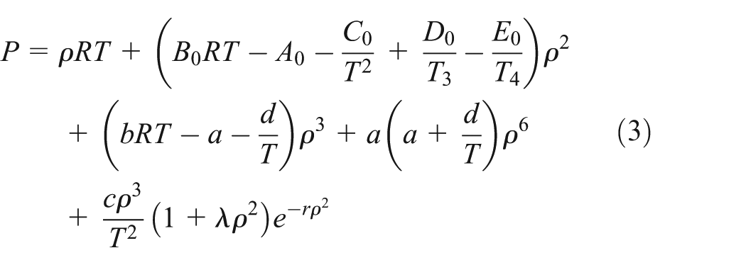
\begin{matrix} P = & ρ RT + (B_{0} RT - A_{0} - \frac{C_{0}}{T^{2}} + \frac{D_{0}}{T_{3}} - \frac{E_{0}}{T_{4}}) ρ^{2} \\ + (bRT - a - \frac{d}{T}) ρ^{3} + a (a + \frac{d}{T}) ρ^{6} \\ + \frac{c ρ^{3}}{T^{2}} (1 + λ ρ^{2}) e^{- r ρ^{2}} \end{matrix}

(3)

The BWRS state equation is not only suitable for both one-component hydrocarbon and one-component non-hydrocarbon gases but also natural gas containing non-hydrocarbon components, but the calculation accuracy is significantly affected by the specific heat capacity. For the calculation of natural gas, in order to expect higher calculation accuracy, it is necessary to provide a reliable heat capacity relationship. It takes more corrections into account and thus introduces more parameters. The BWRS equation is a complex state equation with up to 11 parameters. The more parameters are introduced, the wider the scope of application, but the difficulty in solving and the calculation amount is also larger. The calculation method is more complicated and the calculation speed is slower.^20–22

Gas flow equations

AGA equation

AGA equation is divided into a low-flow turbulent part and a high-velocity turbulent part. Low-flow turbulence part is given as follows

\begin{array}{l} Q_{b} = 38.77 \frac{T_{b}}{P_{b}} {[\frac{P_{1}^{2} - P_{2}^{2} - 0.375 G (h_{2} - h_{1}) \frac{P_{a v g}^{2}}{z_{a v g} T_{a v g}}}{G L T_{a v g} z_{a v g}}]}^{0.5} \\ \times 4 D_{f} \log [\frac{N_{Re}}{1.4126 \sqrt{1 / f}}] \times D^{2.5} \end{array}

(4)

High-velocity turbulent part is given as follows

\begin{array}{l} Q_{b} = 38.77 \frac{T_{b}}{P_{b}} {[\frac{P_{1}^{2} - P_{2}^{2} - 0.375 G (h_{2} - h_{1}) \frac{P_{a v g}^{2}}{z_{a v g} T_{a v g}}}{G L T_{a v g} z_{a v g}}]}^{0.5} \\ \times [4 \log \frac{3.7 D}{k_{e}}] \times D^{2.5} \end{array}

(5)

Colebrook–White equation

The Colebrook–White equation is a general-purpose recommended equation. It combines smooth pipe rules with rough pipeline rules to provide excellent accuracy for a wide range of flow conditions.

Panhandle equation

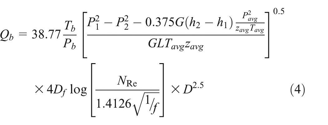
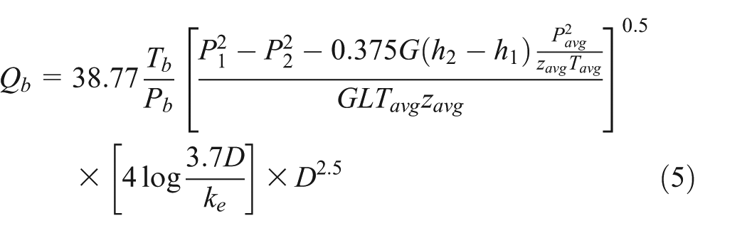
The Panhandle “A” friction coefficient formula has been developed by Panhandle and Eastern Gas Company, and it varies with the Reynolds number. The equation is applied to the design of natural gas pipe diameters from DN150 to DN600 and the Reynolds number from 5,000,000 to 14,000,000. The coefficient of friction can be expressed as follows

\sqrt{1 / f} = 6.872 {(N_{Re})}^{0.0730} E

(6)

where E is an effective coefficient.

Equation selection

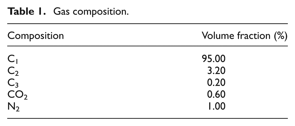
In order to identify the most reasonable state equation and the gas flow equation, according to the three state equations and five gas flow equations, the different calculation results of natural gas (dry gas) under the same temperament condition are discussed. The gas composition and the transport conditions are shown in Tables 1 and 2.

Table 1.

Gas composition.

Composition	Volume fraction (%)
C₁	95.00
C₂	3.20
C₃	0.20
CO₂	0.60
N₂	1.00

Table 2.

Pipeline transportation condition.

Starting point pressure (MPa)	6	Starting point temperature (°C)	25
Transmission capacity (m³/d)	100 × 10⁴	Pipeline length (km)	50
Total heat transfer coefficient of ground temperature (W/m²·C)	1.75	Ambient temperature (°C)	5
Pipe diameter (mm)	219	Wall thickness (mm)	5
Wall roughness (µm)	30	Pipeline efficiency	0.95
Steel grade	X60 (L415)

It can be seen from Figure 1 that the variation trend of the outlet pressure, outlet temperature, and outlet gas velocity curve calculated by different pressure drop formulas are almost the same when different state equations are adopted. The average calculation error is about 1.5% when the formula of Pan (A) and Pan (B) is used as the pressure drop equation. When the other formulas are used, the mean calculation error is about 4.6%. When using the “SAREM” state equation, the calculated results have a big difference with other two state equations, especially the outlet temperature calculation results.

Figure 1.

Outlet parameters change curves: (a) outlet pressure, (b) outlet temperature, and (c) outlet gas velocity.

BWRS equation and Peng–Robinson equation are recommended in the calculation of CBM gathering and transportation. The Colebrook–White equation is recommended for gas flow equation.

Equations in PIPEPHASE software

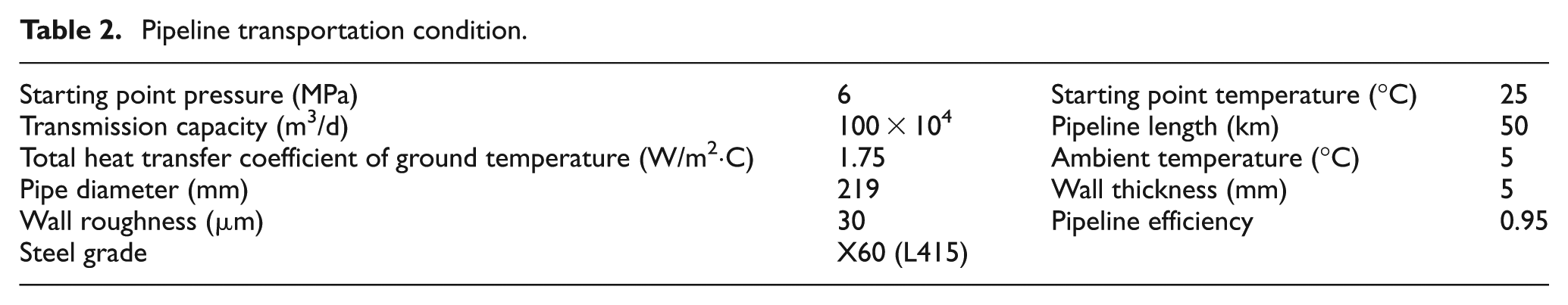
PIPEPHASE is a rigorous multiphase flow simulator for oil and gas production networks, and piping and distribution system calculations. It has a strong advantage in the calculation of two-phase flow. “SRK,”“SRK-KD,”“SRK-HV,”“SRK–Panagiotopoulos–Reid,”“SRK-SIMSCI,”“Peng–Robinson,”“PR-HV,”“PR-Panagiotopoulos-Reid,” and “BWRST,” are suitable for the calculation of the natural gas gathering and transportation in PIPEPHASE. They also provide the equations of “Begs and Brill,”“Beggs and Brill–Moody,”“Beggs and Brill–Moody–Hagedorn and Brown,”“Mukherjee and Brill,”“Mukherjee and Brill–Eaton,”“Eaton–Flannigan,”“Dukler–Flannigan,”“Dukler–Eaton–Flannigan,”“Olimens,”“Ansari,”“Duns and Ros,”“Aziz,”“Orkiszewski,”“Angel–Welchon–Ross,” and other 26 kinds of pressure drop formulas. Gas composition and the transport conditions are shown in Tables 3 and 4.

Table 3.

Gas composition.

Composition	Volume fraction (%)
C₁	98.70
C₂	0.40
CO₂	0.20
N₂	0.30
H₂O (saturated water)	0.40

Table 4.

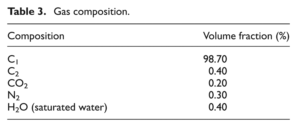
Pipeline transportation condition.

Starting point pressure (MPa)	0.15	Starting point temperature (°C)	25
Transmission capacity (m³/d)	1 × 10⁴	Pipeline length (km)	10
Total heat transfer coefficient of ground temperature (W/m²·C)	1.75	Ambient temperature (°C)	5
Pipe diameter (mm)	160	Wall thickness (mm)	14.6
Wall roughness (µm)	30	Pipeline efficiency	0.95
Pipe material	PE

It can be seen from Figure 2 that the calculated outlet pressure and temperature variation range are very small under the condition of using different state equations and the pressure drop formula, the nine curves almost completely coincide, and the difference is not obvious. It is suggested to use the BBM pressure drop formula under the default SRK state equation to calculate the pressure drop of pipeline, which can get better accuracy in a wide range of variation.

Figure 2.

Outlet parameters change curves: (a) outlet pressure and (b) outlet temperature.

Analysis of TGNET and PIPEPHASE software adaptability

In order to compare the adaptability of TGNET and PIPEPHASE software to the hydraulic analysis of CBM field, using an example, two kinds of software were used to simulate the example, and the results were compared with the field data. Based on a section of gas-collecting branch, the distance relation and connection relation are shown in Figure 3. Gas composition and the transport conditions are shown in Tables 3 and 4. PIPEPHASE software uses SRK state equation and “Beggs and Brill–Moody” pressure drop formula, TGNET software uses BWRS state equation and Colebrook pressure drop formula. Simulated results of the PIPEPHASE and TGNET software are shown in Table 5. The boundary conditions of “wellhead-fixed flow (maximum flow) and station-fixed pressure (minimum pressure)” are used.

Figure 3.

Distance relation and connection relation.

Table 5.

Pipeline transportation condition.

Starting point pressure (MPa)	0.5	Starting point temperature (°C)	25
Transmission capacity (m³/d)	1 × 10⁴	Pipeline length (km)	10
Total heat transfer coefficient of ground temperature (W/m²·C)	1.75	Ambient temperature (°C)	5
Pipe diameter (mm)	110	Wall thickness (mm)	10.0
Wall roughness (µm)	30	Pipeline efficiency	0.95
Pipe material	PE

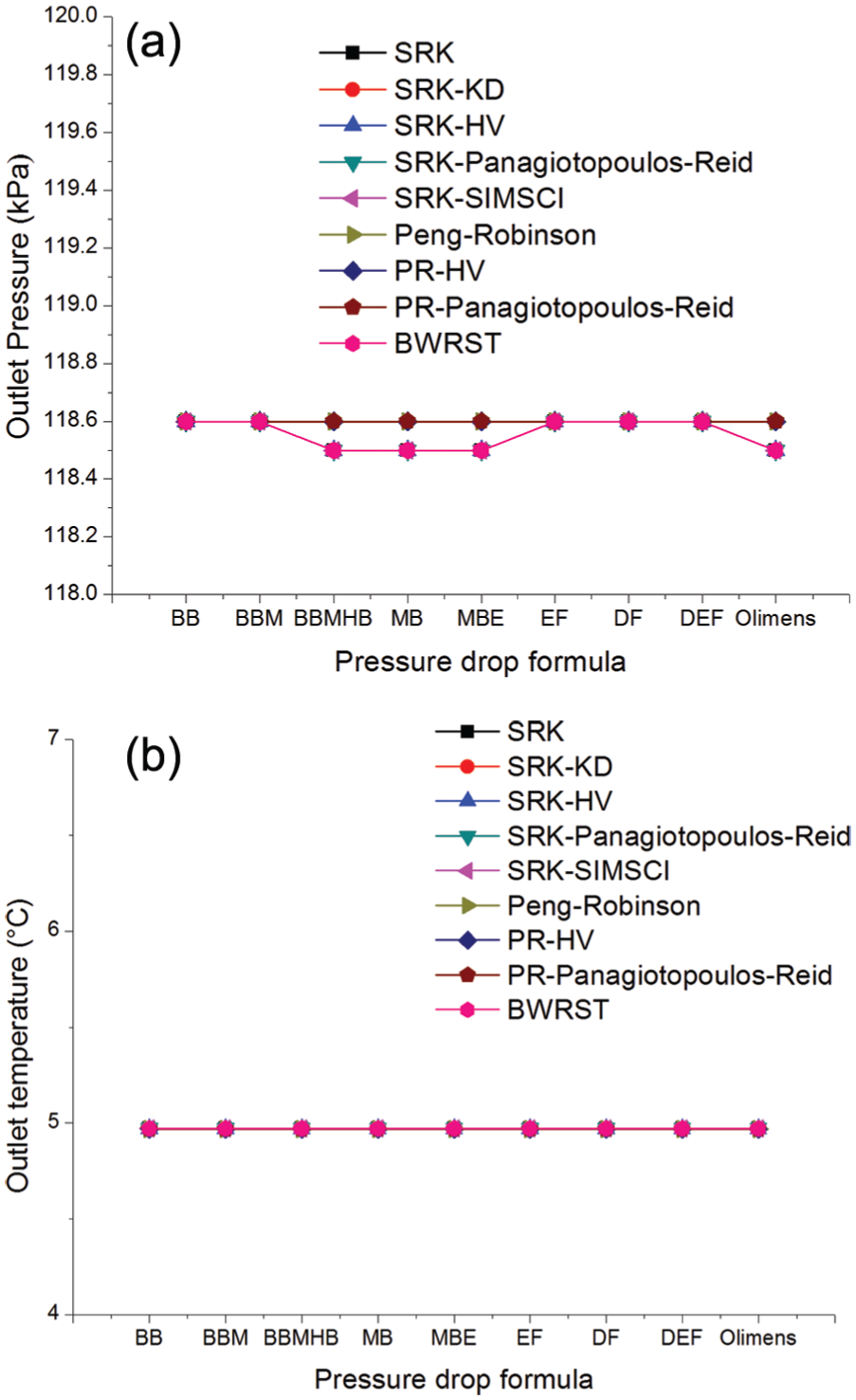
From Figure 4, it can be seen that the difference of wellhead pressure calculated by PIPEPHASE software and TGNET software is small. When compared with the actual wellhead pressure, the PIPEPHASE software calculation results are closer to the actual value than the wellhead pressure value calculated by TGNET software, which indicates that the PIPEPHASE software is relatively more practical in calculating low-pressure CBM with saturated water.

Figure 4.

Simulated relative error results of the PIPEPHASE and TGNET software.

PIPEPHASE software has a good agreement with the actual situation in the calculation of low-pressure CBM pipeline network, and its calculation results are more reliable. At the same time, in the simulation, we must integrate terrain, volume, diameter, distance, and other factors to get more realistic results. Therefore, in the low-pressure CBM gathering process calculation, it is recommended to use PIPEPHASE software for calculation.

Analysis of factors affecting pressure drop

How to make full use of wellhead pressure and maximize the ability of wellhead pressure is an important link in CBM surface engineering optimization. In the gathering and transportation process, the pipeline transportation capacity and the outlet pressure drop are affected by the fluid inlet temperature, inlet pressure, ground temperature, total heat transfer coefficient of the ground temperature, flow rate, transport distance, roughness of the pipe wall, the pipeline efficiency, and water content of raw gas. The influence of various factors on the pressure drop was calculated and analyzed by PIPEPHASE software.

In accordance with the temperament parameters and transport conditions shown in Tables 3 and 5, the SRK state equation and BBM pressure drop formula were used to calculate the straight pipeline as an example to determine the effect of each factor on the gathering pipeline.

Inlet temperature

Based on the conditions in Tables 3 and 5, the inlet temperature of the fluid was changed from 10°C to 50°C, and the influence of the factors on the pressure drop was investigated. It can be seen from Figure 5 that the inlet temperature has little effect on the pressure drop of the pipeline (from 10°C to 50°C, the maximum pressure drop is only 0.4 kPa), it can be negligible. While the outlet temperature decreases with the increase in inlet temperature, the change range is very small. This occurs because the temperature difference between the inlet and the ground increases as the inlet temperature increases, increasing the heat transfer between the pipeline and the soil, resulting in a slight difference in the outlet temperature.

Figure 5.

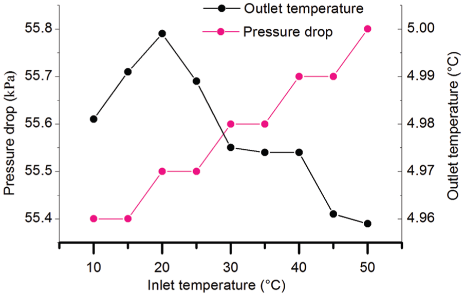
Pressure drop curves for different inlet temperatures.

Inlet pressure

The inlet pressure was changed from 300 to 1500 kPa, and the influence of this factor on the pressure drop was investigated. It can be seen from Figure 6 that the outlet pressure and the pressure drop along the pipeline increase and decrease, respectively, with the increase in the inlet pressure. At the same time, when the inlet pressure varied from 300 to 550 kPa, the outlet pressure increased linearly with the increase in the inlet pressure, but the pressure drop along the pipeline decreased rapidly with the increase in the inlet pressure. Subsequently, with the further increase in the inlet pressure, the outlet pressure gradually increased. The pipeline along the pressure drop trend becomes smaller. It can be concluded that the use of higher inlet pressure is conducive to improve the outlet pressure, reducing the pressure drop along the pipeline, reducing pressure loss, which will help pipeline transportation.

Figure 6.

Pressure drop curves for different inlet pressures.

Ground temperature

Change the ground temperature (from −5°C to 5°C) to investigate the influence of the factors on the pressure drop of the pipeline. It can be seen from Figure 7 that the outlet pressure gradually increases with the increase in the buried temperature. When the temperature rises from −5°C to 0°C, the outlet pressure rises rapidly. After 0°C, the outlet pressure tends to be gentle and no obvious change is observed. Similarly, with the increase in the ground temperature, the outlet pressure increases, and the pressure drop along the pipeline decreases, and tends to be gentle. Therefore, in order to reduce the pressure drop along the pipeline to improve the outlet pressure and increase pipeline capacity, pipeline laying ground temperature should be above 0°C.

Figure 7.

Pressure drop curves for different ground temperatures.

Total heat transfer coefficient of the ground temperature

The total heat transfer coefficient (K in the range of 1–1.9) was changed to investigate the influence of the factor on the pressure drop of the pipeline. In addition, the influence of the total heat transfer coefficient of ground temperature on the pressure drop of the pipeline was calculated under the conditions of maximum pipe flow rate and different ground temperatures (5°C and 0°C).

It can be seen from Figure 8 that with the increase in the total heat transfer coefficient of the ground temperature, there is no obvious change in the outlet pressure and the pipeline pressure drop, and the outlet temperature does not fluctuate too much.

Figure 8.

Pressure drop curves for different total heat transfer coefficients of the ground temperature.

It can be seen from Figure 9 that the outlet pressure at 0°C is higher than the outlet pressure at 5°C, and the pressure drop is lower than that at 5°C. From the whole trend, regardless of the ground temperature, the outlet pressure of the pipeline increases with the increase in the total heat transfer coefficient of ground temperature, and the pressure drop also decreases. In the case of the same total heat transfer coefficient of ground temperature, the ground temperature is low and the pressure drop of the pipeline is small.

Figure 9.

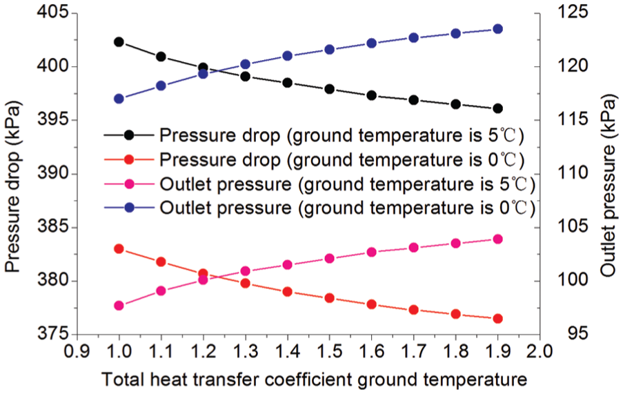
Influence of total heat transfer coefficient on the pressure drop of pipeline at different ground temperatures.

Flow rate

Change the flow rate (from 5000 to 15,000 m³/d) and investigate the influence of the factors on the pressure drop of the pipeline. It can be seen from Figure 10 that the trend of the pressure drop and the outlet pressure of the pipeline gradually increase and decrease, respectively, as the flow rate increases. There is no obvious fluctuation in the whole trend; it is a law which changes linearly with the change in the flow rate. It can be concluded that the flow rate has an effect on the pressure drop and the outlet pressure, but its effect does not cause appreciable fluctuations in the pressure drop and the outlet pressure.

Figure 10.

Pressure drop curves for different flow rate.

Transport distance

The transport distance (from 3 to 20 km) was changed to investigate the influence of the factor on the pressure drop of the pipeline. It can be seen from Figure 11 that the trend of the pressure drop and the outlet pressure of the pipeline gradually increase and decrease, respectively, as the transport distance increases. The whole trend has no obvious fluctuation, and it is a law which changes linearly with the change in the conveying distance.

Figure 11.

Pressure drop curves for different transport distances.

Roughness of the pipe wall

The roughness of the pipe wall (from 0.01 to 0.05 mm) was changed to investigate the influence of the factor on the pressure drop of the pipeline. In addition, the inlet pressure was controlled at 80, 200, 500, 1000, and 1500 kPa, the wall roughness was kept at 0.03 mm, and the other conditions were fixed. The maximum outlet flow rate of the pipeline under different inlet pressures was calculated as 7800, 2.24 × 10⁴, 3.8 × 10⁴, and 5.31 × 10⁴ m³/d. Then, adjust the pipe wall roughness (from 0.01 to 0.03 mm) and investigate the influence of the factors on the pressure drop of the pipeline.

It can be seen from Figure 12 that under certain inlet pressure conditions, the pipe pressure drop increases with the increase in pipe wall roughness. It can be seen from Figure 13 that the slope of the pressure drop curve increases with the increase in inlet pressure, that is, the variation range of pressure drop of the pipeline increases rapidly with the increase in the roughness of the pipe wall. When the inlet pressure is 200 kPa, the slope of the curve is K = 4.5, the whole curve trend is gentle, and the pressure drop of the pipeline decreases with the increase in the roughness of the pipe wall, indicating that at low pressure, the influence of the roughness of the pipe wall on the normal transportation is also small. When the inlet pressure is 1500 kPa, the slope of the pipeline pressure drop curve is K = 140, and the curve shows a rapid upward trend with the increase in the roughness of the pipe wall; it is shown that the roughness of the pipe wall has a great influence on the normal transportation of pipeline at higher pressure. It can be concluded that the higher the pipeline delivery pressure, the greater the influence of pipe wall roughness on the pressure drop of pipeline transportation, and the greater the pressure loss.

Figure 12.

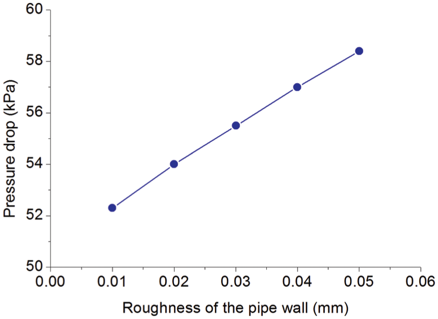
Pressure drop curves for different roughness of the pipe wall.

Figure 13.

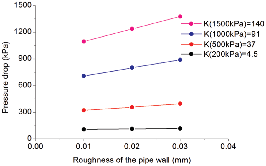
Pressure drop curves for different roughness of the pipe wall and different inlet pressures.

Pipeline efficiency

Under the condition of inlet pressure of 500 kPa, the outlet pressure is more than 100 kPa, the pipeline length is 10 km, the diameter is 110 mm, and the maximum pipeline capacity of pipeline is 2.24 × 10⁴ m³/d. Under this condition, the efficiency of pipeline transportation is changed, and the effect of pipeline efficiency on the pressure drop is investigated. In addition, under the condition of inlet pressure of 200, 1000, and 1500 kPa, the other conditions are not changed, the efficiency of pipeline transportation is adjusted (from 95% to 100%), and the influence of this factor on the pressure drop of pipeline is investigated.

It can be seen from Figure 14 that the trend of the pressure drop and the outlet pressure of the pipeline gradually decrease and increase, respectively, with the increase in the pipeline efficiency. The whole trend is a law of linear change with the change in the efficiency of pipeline transportation.

Figure 14.

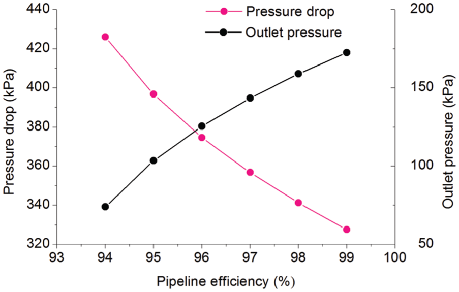
Pressure drop curves for different pipeline efficiencies.

It can be seen from Figure 15 that under certain inlet pressure conditions, the pressure drop of the pipeline decreases with the increase in the pipeline efficiency. At the same time, with the increase in the inlet pressure, the pressure drop varies with the pipeline efficiency and the change tendency is smaller than that of wall roughness. When the inlet pressure is 200 kPa, the slope of the curve is K = −3.5; when the inlet pressure is 1500 kPa, the slope of the pipeline pressure drop curve is K = −50, and its slope is smaller than that of the pipe wall roughness curve. It can be explained that the higher the inlet pressure, the greater the effect of pipeline efficiency on pipeline pressure drop.

Figure 15.

Pressure drop curves for different pipeline efficiencies and different inlet pressures.

Water content of raw gas

The water content of raw gas (from 0.1% to 1.0%) was changed to investigate the influence of the factor on the pressure drop of the pipeline.

It can be seen from Figure 16 that the outlet pressure and the pressure drop along the pipeline will show significant fluctuation as the water content of the raw gas increases. When the water content in the feed gas is 0.374% (saturated water content) and near the water content (4%), the change of water content of the raw gas has little effect on the outlet pressure and the pressure drop along the pipeline; but when the water content of the raw gas varies between 0.4% and 0.6%, the outlet pressure decreases rapidly and the pressure drop increases rapidly along with the increase in the water content. When the water content of raw material gas is between 0.7% and 1%, the outlet pressure and the pressure drop along the pipeline trend tend to be gentle, and no more significant fluctuations are observed. It can be concluded that under certain transport conditions, the lower the moisture content of raw gas, the higher the outlet pressure, and the lower the pressure drop along the pipeline, the less the pressure loss, and the better the transportation.

Figure 16.

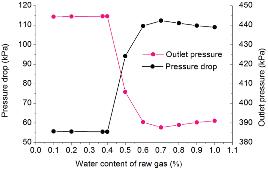
Pressure drop curves for different water content of raw gas.

Conclusion

The main purpose of this article was to identify the hydraulic adaptability of the CBM field and analyze the pressure drop factors. Based on the above-mentioned analysis, the following conclusions can be drawn:

PIPEPHASE software is recommended for CBM hydraulic calculation.

In PIPEPHASE software, it is recommended to use the SRK state equation and the BBM pressure drop formula for the hydraulic calculation of the low-pressure gas production pipeline network in the CBM field.

In order to reduce the pressure drop along the pipeline, increase the outlet pressure, increase the pipeline capacity, and lay the pipeline under permafrost layer below (0°C or more).

The higher the pipeline delivery pressure, the greater the influence of pipe wall roughness on the pressure drop of pipeline transportation, and the greater the pressure loss.

The higher the inlet pressure of the pipeline, the more obvious the effect of pipeline efficiency on the pressure drop of the pipeline. The inlet pressure and the pipeline efficiency should be reasonably determined.

The use of higher inlet pressure helps to improve the outlet pressure, reducing the pressure drop along the pipeline, reducing pressure loss, which will help pipeline transportation.

Under certain transport conditions, the lower water content of raw gas is conducive to increase the outlet pressure, and reducing the pressure drop along the pipeline to reduce the pressure loss is conducive to transportation.

Footnotes

Academic Editor: Kun Huang

Declaration of conflicting interests

The author(s) declared no potential conflicts of interest with respect to the research, authorship, and/or publication of this article.

Funding

The author(s) received no financial support for the research, authorship, and/or publication of this article.

References

Zhao

Hui

. Difference between PIPEPHASE and TGNET in the simulation of the low pressure gathering system in the coal-bed methane field. Petrol Plann Eng 2013; 24: 32–34.

Mukherjee

Brill

JP.

Liquid holdup correlations for incline two-phase flow. J Petrol Technol 1983; 35: 1003–1008.

Lockhart

Martinelli

RC.

Proposed correlation of data for isothermal two-phase, two-component flow in pipes. Chem Eng Prog 1949; 45: 39–48.

Orkiszewski

Predicting two-phase pressure drops in vertical pipe. J Petrol Technol 1967; 19: 829–838.

Mukherjee

Brill

JP.

Empirical equations to predict flow patterns in two-phase inclined flow. Int J Multiphas Flow 1985; 11: 299–315.

Martin

Peters

The application of Newton’s method to network analysis by digital computer. J Inst Water Eng 1963; 17: 115–129.

Collins

Johnson

RL.

Finite-element method for water-distribution networks. J Am Water Works Ass 1975; 67: 385–389.

Wood

Charles

COA

. Hydraulic network analysis using linear theory. J Hydr Eng Div 1972; 98: 1157–1170.

Rush

Huebler

Smith

RW.

Integrating microelectronics into gas distribution. Boca Raton, FL: CRC Press, 1987.

10.

Smith

Zhang

China compressor operations optimized with help of pipeline studio model. Pipeline Gas J 2003; 230: 73–74.

11.

Ang

Jowitt

PW.

Solution for water distribution systems under pressure-deficient conditions. J Water Res Pl 2006; 132: 175–182.

12.

Tang

SN.

Hydraulic analysis and optimal operation of city gas pipeline network in case of emergency. Master’s Thesis, Harbin Institute of Technology, Harbin, China, 2015.

13.

Hagedorn

Brown

KE.

Experimental study of pressure gradients occurring during continuous two-phase flow in small-diameter vertical conduits. J Petrol Technol 1965; 17: 475–484.

14.

Eaton

Knowles

Silberbrg

IH.

The prediction of flow pattern, liquid holdup and pressure losses occurring during continuous two-phase in horizontal pipelines. J Petrol Technol 1967; 19: 815–828.

15.

Zhang

Wang

Tian

Influence of undulating terrains on operation conditions of condensate gas gathering lines. Nat Gas Ind 2013; 33: 108–113.

16.

Wang

Zeng

ZQ.

Static and dynamic emulation of natural gas pipeline network. Nat Gas Ind 1995; 15: 59–63.

17.

Balakhrisna

Ghosh

Das

. Oil–water flows through sudden contraction and expansion in a horizontal pipe–phase distribution and pressure drop. Int J Multiphas Flow 2010; 36: 13–24.

18.

Cao

Feng

SC.

Development of Pinghu-Shanghai gas pipeline simulator. Oil Gas Storage Transp 1997; 16: 16–21.

19.

Tian

Chen

Mei

. Optimization of ground surface gathering and transportation process in the Fanzhuang block, southern Qinshui Basin. Nat Gas Ind 2011; 31: 30–33.

20.

Wang

Liu

Wang

. CBM ground technology in Qinshui Basin. Nat Gas Ind 2008; 28: 109–110.

21.

Xue

Wang

. Process optimization of surface gathering system: case history of the Fanzhuang Block in the coalbed methane gas fields, Qinshui Basin. Nat Gas Ind 2010; 30: 87–90.

22.

Xue

Wang

. Optimization of flow line network: case history of the Fanzhuang block in the coalbed methane gas fields, Qinshui Basin. Nat Gas Ind 2010; 30: 91–93.

Analysis on hydraulic adaptability and pressure drop factors of low-pressure pipe network in coal-bed methane field

Abstract

Keywords

Introduction

Basic theory

Equations in TGNET software

State equations

Sarem state equation

Peng–Robinson state equation

BWRS state equation

Gas flow equations

AGA equation

Colebrook–White equation

Panhandle equation

Equation selection

Equations in PIPEPHASE software

Analysis of TGNET and PIPEPHASE software adaptability

Analysis of factors affecting pressure drop

Inlet temperature

Inlet pressure

Ground temperature

Total heat transfer coefficient of the ground temperature

Flow rate

Transport distance

Roughness of the pipe wall

Pipeline efficiency

Water content of raw gas

Conclusion

Footnotes

Declaration of conflicting interests

Funding

References