Sage Journals: Discover world-class research

Abstract

This article deals with the propagation of fundamental plane mode in pentafurcated waveguide structure with soft–hard boundaries. Three semi-infinite ducts are located inside an infinite waveguide. In particular, we aim to find the reflected field amplitude for the underlying problem by using the standard mode-matching approach. We also present some numerical illustrations by determining the reflected field amplitude for different dimensions of the pentafurcated waveguide structures. Such investigations are useful in the reduction of noise effects generated through variety of mechanisms.

Keywords

Scattering reflected field soft–hard pentafurcated waveguide energy balance

Introduction

A major concern in the developed world is how to reduce structural vibration, and harmful and unwanted noise in many technical and industrial complicated devices. The duct outlet is an important research area of noise reduction and relevant for many scientists, physicists, engineers, and applied mathematicians. The propagation and scattering of acoustic waves in a waveguide with different types of boundary conditions (such as soft, hard, and impedance) can be designed to form various types of physical structures.

The mathematical models for such structures involve essential difficulties in the form of non-linear dispersion relations and unusual orthogonal properties of eigenfunctions. Andronov and Belinsky¹ demonstrated the concept of the eigenfunctions arising for large number of waveguide problems which display unusual orthogonality properties. Different types of structures have been considered by Lawrie and colleagues^2–4 where mode-matching technique is applied to get solutions there by developing new orthogonality relations. Lawrie⁵ also explained an analytical mode-matching technique which is suitable for the solution of the geometries involving scattering in three-dimensional waveguide with flexible wall. Ammari et al.⁶ presented the scattering of electromagnetic waves by a thin dielectric planar structure. They also described the a method which can be viewed as a computational approach that potentially simplifies scattering calculations for problems involving thin scatterers. Ammari et al.⁷ have also developed a solution to the problem of reconstructing the spatial support of noise sources from boundary measurements using cross-correlation techniques. They discussed the case where the noise sources are spatially correlated.

Many researchers solved various type of geometries by integral transform and Jones’ method based on Wiener–Hopf technique. The solution involves the complicated factors or split functions when we use Wiener–Hopf technique. Sometimes, this technique leads to matrix Wiener–Hopf problems which are very difficult to handle. Nawaz and Ayub⁸ discussed the closed-form solution of electromagnetic wave diffraction problem in a homogeneous bi-isotropic medium. Nawaz et al.⁹ explained the acoustic propagation in two-dimensional (2D) waveguide for membrane-bounded ducts. Buyukaksoy et al.¹⁰ presented the Wiener–Hopf analysis for the propagation of waves in a bifurcated cylindrical waveguide with wall impedance discontinuity. Buyukaksoy et al.¹¹ also explained the scattering of plane waves by a junction of a transmission and soft–hard half planes by applying the Wiener–Hopf technique. Buyukaksoy and Cinar¹² analyzed the solution of a matrix Wiener–Hopf equation connected with the plane wave diffraction by an impedance-loaded parallel-plate waveguide. Rawlins¹³ also obtained an exact solution of a bifurcated circular waveguide problem by applying with the same technique. Hassan and Rawlins¹⁴ explained the propagation of sound radiations in a planar trifurcated lined duct and obtained a closed-form solution. Ayub and colleagues^15–17 analyzed the diffraction of dominant mode on acoustic wave propagation in a trifurcated lined duct with different boundary conditions. They have also presented solutions by using the Wiener–Hopf technique.

The eigen mode-matching method is conceptually simple, powerful, and straight forward as compared to other techniques like the Wiener–Hopf and Green function. Mode-matching method leads to numerically efficient system of equations which can be truncated numerically. That is why, this method has been used by many researchers in an enormous variety of disciplines to deal with wide range of geometries with different boundary conditions. If the field equation is not higher than second order, then the solutions can be obtained by separation of variable method in terms of an eigenfunction expansions for the problems which consist of different soft, hard, and impedance walls of the duct. Hassan¹⁸ has discussed a trifurcated problem with soft–hard boundaries using the eigenfunction expansion method.

Keeping in view the above-mentioned background, we consider here pentafurcated problem with combination of soft–hard boundary conditions on plates. The alternate soft lining is taken to simplify the analysis and to get a good first-hand approximation of the reflected field amplitude in actual systems. This prototype model will be helpful to tackle with more general conditions. We divide our geometry into six regions. The potential solution is obtained in each region by using separation of variables. The solutions involve an infinite number of modes which are matched by using continuity of pressure and velocity of potential of each region across boundary at $x = 0$ . The orthogonality relations permit the given problem to be reduced in the form of an infinite systems of linear algebraic equations. This infinite systems of equations are solved by applying MATLAB programming. The linear systems of equations converge slowly, so we truncate systems of equations in our calculation and estimate the solution. We present the graphical representation of the reflected field $| R |$ against the wave number k for various dimensions of the waveguide. The related work has been discussed by Hassan et al.¹⁹ In this, they have presented the reflected field analysis for pentafurcated waveguide having hard plates. We also give the comparison of the radiated acoustic power down the guide which is proportional to the $(1 - | R |^{2})$ between the current problem and the hard pentafurcated duct problem.¹⁹ This research work will be helpful for engineers in designing practical exhaust systems.

This article is organized as follows. The model problem is formulated in section “Formulation of pentafurcated waveguide,” whereas mode-matching solutions are presented in section “Solution of the pentafurcated waveguide.” Some numerical illustrations are described in section “Numerical results,” and the results are summarized in section “Summary.”

Formulation of pentafurcated waveguide problem

We shall consider the scattering of an incident plane wave from any source propagating toward the open end of the middle region $(| y | < a, x < 0)$ of a two-dimensional pentafurcated duct problem as shown in Figure 1. The pentafurcated waveguide is designed such that two soft and two hard semi-infinite plates are located inside two infinite plates. An infinite hard plate is located at $y = d$ and other infinite soft plate is located below the x-axis at $y = - d$ . The acoustic pressure P is defined such that

P = - ρ_{o} \frac{\partial φ}{\partial t}

(1)

where $ρ_{o}$ represents the density in equilibrium state. The scalar potential $φ (x, y, t)$ in term of velocity vector $\vec{u}$ is defined as

\vec{u} = g r a d (φ)

(2)

where $φ$ satisfies the following wave equation

\nabla^{2} φ = (1 / c^{2}) φ_{t t}

(3)

Figure 1.

Schematic diagram of the pentafurcated duct.

While considering the time harmonic solution of the form

φ (x, y, t) = Re [v (x, y) e^{- i w t}]

(4)

equation (3) is identically satisfied which eventually results into a well-known Helmholtz equation in 2D, that is

(\nabla^{2} + k^{2}) v (x, y) = 0

(5)

within the duct, where $k = \frac{w}{c}$ is the wave number, w is the angular frequency and c is the speed of sound. We will solve the problem subjected to the following boundary conditions

v (x, y) = 0, y = - d, - \infty < x < \infty

(6)

v_{y} (x, y) = 0, y = - b, - \infty < x < 0

(7)

v (x, y) = 0, y = - a, - \infty < x < 0

(8)

v_{y} (x, y) = 0, y = a, - \infty < x < 0

(9)

v (x, y) = 0, y = b, - \infty < x < 0

(10)

v_{y} (x, y) = 0, y = d, - \infty < x < \infty

(11)

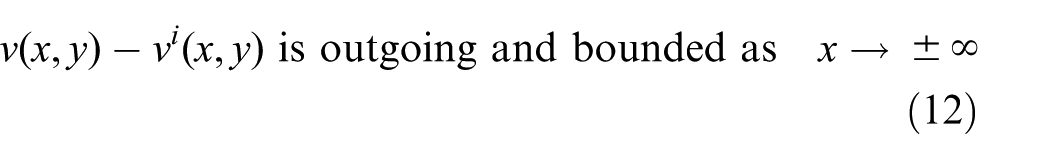
The wave field satisfies the radiation conditions

v (x, y) - v^{i} (x, y) is outgoing and bounded as x \to \pm \infty

(12)

which simply ensures the boundedness of the obtained solution.

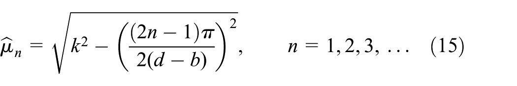
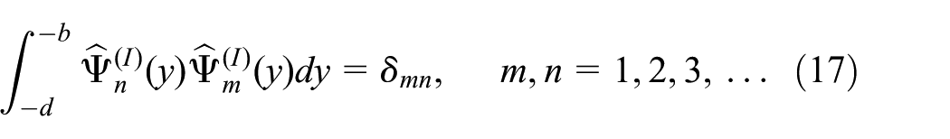
Region I ${- d \leq y \leq - b, x < 0}$

We employ the method of separation of variables to solve the given problem in various regions by following the standard procedure from Mei²⁰ and Linton and Mclver²¹ in terms of eigenfunctions expansion. The potential solution of equation (5) in this region can be written as

v (x, y) = \sum_{n = 1}^{\infty} B_{n} e^{- i {\hat{μ}}_{n} x} {\hat{Ψ}}_{n}^{(I)} (y)

(13)

which satisfies equations (6) and (7) and radiation condition (12), where $B_{n}$ is the amplitude of the transmitted field in region I.

The eigenvalues $μ_{n} = \frac{(2 n - 1) π}{2 (d - b)}$ are the solution of the following relation

\cos μ_{n} (d - b) = 0, n = 1, 2, 3, \dots

(14)

The associated eigenvalues are

{\hat{μ}}_{n} = \sqrt{k^{2} - {(\frac{(2 n - 1) π}{2 (d - b)})}^{2}}, n = 1, 2, 3, \dots

(15)

with $0 < Im ({\hat{μ}}_{1}) < Im ({\hat{μ}}_{2}) \dots$ and $Re ({\hat{μ}}_{n}) > 0$ .

The eigenfunctions ${\hat{Ψ}}_{n}^{(I)} (y)$ in this region are defined as

{\hat{Ψ}}_{n}^{(I)} (y) = \sqrt{\frac{2}{(d - b)}} \sin μ_{n} (y + d)

(16)

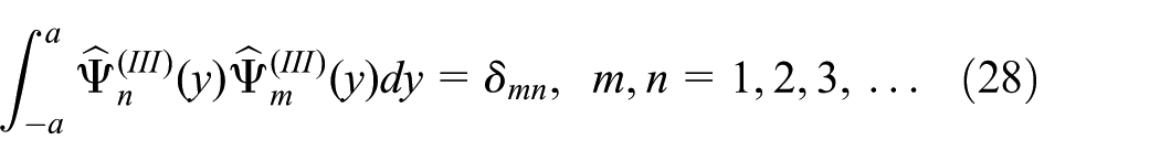
which satisfy the orthonormal relation

\int_{- d}^{- b} {\hat{Ψ}}_{n}^{(I)} (y) {\hat{Ψ}}_{m}^{(I)} (y) dy = δ_{mn}, m, n = 1, 2, 3, \dots

(17)

where $δ_{mn}$ is Kronecker delta defined by

δ_{mn} = {\begin{matrix} 0, & m \neq n \\ 1, & m = n \end{matrix}

(18)

Region II ${- b$ $\leq y$ $\leq - a, x < 0}$

The potential solution of equation $(5)$ in this region is given by

v (x, y) = \sum_{n = 1}^{\infty} D_{n} e^{- i {\hat{α}}_{n} x} {\hat{Ψ}}_{n}^{(II)} (y)

(19)

which satisfies equations (7) and (8) and radiation condition (12), where $D_{n}$ are the amplitudes of transmitted field in the region II.

The eigenvalues $α_{n} = \frac{(2 n - 1) π}{2 (b - a)}$ satisfy the equation

\cos α_{n} (b - a) = 0, n = 1, 2, 3, \dots

(20)

The associated eigenvalues are

{\hat{α}}_{n} = \sqrt{k^{2} - {(\frac{(2 n - 1) π}{2 (b - a)})}^{2}}, n = 1, 2, 3, \dots

(21)

with $0 < Im ({\hat{α}}_{1}) < Im ({\hat{α}}_{2}) \dots$ and $Re ({\hat{α}}_{n}) > 0$ .

The eigenfunctions ${\hat{Ψ}}_{n}^{(II)} (y)$ in this region are given by

{\hat{Ψ}}_{n}^{(II)} (y) = \sqrt{\frac{2}{(b - a)}} \sin α_{n} (y + a)

(22)

The eigenfunctions satisfy the orthonormal relation

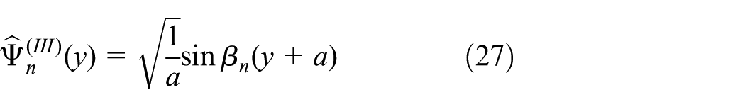
\int_{- b}^{- a} {\hat{Ψ}}_{n}^{(II)} (y) {\hat{Ψ}}_{m}^{(II)} (y) dy = δ_{mn}, m, n = 1, 2, 3, \dots

(23)

Region III ${- a$ $\leq y$ $\leq a, x < 0}$

The potential solution of equation (5) in region III is defined as

v (x, y) = \sum_{n = 1}^{\infty} F_{n} e^{- i {\hat{β}}_{n} x} {\hat{Ψ}}_{n}^{(III)} (y) + e^{{\hat{β}}_{1} x} {\hat{Ψ}}_{1}^{(III)} (y)

(24)

which also satisfies equations (8) and (9) and radiation condition (12), where $F_{n}$ is the amplitude of the reflected field in region III. The incident wave $e^{i {\hat{β}}_{1} x} {\hat{Ψ}}_{1}^{(III)} (y)$ is excited in the lowest mode propagating from $x = - \infty$ .

The eigenvalues $β_{n} = \frac{(2 n - 1) π}{4 a}$ which are the roots of equation

\cos (β_{n} 2 a) = 0, n = 1, 2, 3, \dots

(25)

The associated eigenvalues are

{\hat{β}}_{n} = \sqrt{k^{2} - {(\frac{(2 n - 1) π}{4 a})}^{2}}, n = 1, 2, 3, \dots

(26)

with $0 < Im ({\hat{β}}_{1}) < Im ({\hat{β}}_{2}) \dots$ and $Re ({\hat{β}}_{n}) > 0$ .

The eigenfunctions ${\hat{Ψ}}_{n}^{(III)} (y)$ in this region are given by

{\hat{Ψ}}_{n}^{(III)} (y) = \sqrt{\frac{1}{a}} \sin β_{n} (y + a)

(27)

which satisfies

\int_{- a}^{a} {\hat{Ψ}}_{n}^{(III)} (y) {\hat{Ψ}}_{m}^{(III)} (y) dy = δ_{mn}, m, n = 1, 2, 3, \dots

(28)

Region IV ${a$ $\leq y$ $\leq b, x < 0}$

The general potential solution of equation (5) in region IV is defined as

v (x, y) = \sum_{n = 1}^{\infty} H_{n} e^{- i {\hat{α}}_{n} x} {\hat{Ψ}}_{n}^{(IV)} (y)

(29)

which satisfies equations (9), (10) and radiation condition (12), where $H_{n}$ are the amplitudes of transmitted field in the region IV.

We define the vertical eigenfunctions region IV as

{\hat{Ψ}}_{n}^{(IV)} (y) = \sqrt{\frac{2}{(b - a)}} \sin α_{n} (y - b)

(30)

The eigenfunctions ${\hat{Ψ}}_{n}^{(IV)} (y)$ satisfy the orthonormal relation

\int_{a}^{b} {\hat{Ψ}}_{n}^{(IV)} (y) {\hat{Ψ}}_{m}^{(IV)} (y) dy = δ_{mn}, m, n = 1, 2, 3, \dots

(31)

Region V ${b$ $\leq y$ $\leq d, x < 0}$

The general potential solution of equation (5) in this region is defined as

v (x, y) = \sum_{n = 1}^{\infty} J_{n} e^{- i {\hat{μ}}_{n} x} {\hat{Ψ}}_{n}^{(V)} (y)

(32)

which satisfies equations (10) and (11) and radiation condition (12), where $J_{n}$ is the amplitude of the transmitted field in region V.

We define the vertical eigenfunctions in region V as

{\hat{Ψ}}_{n}^{(V)} (y) = \sqrt{\frac{2}{(d - b)}} \sin μ_{n} (y - b)

(33)

The eigenfunctions ${\hat{Ψ}}_{n}^{(V)} (y)$ satisfy the orthonormal relation

\int_{b}^{d} {\hat{Ψ}}_{n}^{(V)} (y) {\hat{Ψ}}_{m}^{(V)} (y) dy = δ_{mn}, m, n = 1, 2, 3, \dots

(34)

Region VI ${- d$ $\leq y$ $\leq d, x > 0}$

The general potential solution of equation (5) in region VI is defined as

v (x, y) = \sum_{n = 1}^{\infty} L_{n} e^{i {\hat{λ}}_{n} x} {\hat{Ψ}}_{n}^{(VI)} (y)

(35)

which satisfies equations (6) and (11) and radiation condition (12),where $L_{n}$ is the amplitude of the transmitted field.

The eigenvalues $λ_{n} = \frac{(2 n - 1) π}{4 d}$ satisfy the equation

\cos (λ_{n} 2 d) = 0, n = 1, 2, 3, \dots

(36)

The associated eigenvalues are

{\hat{λ}}_{n} = \sqrt{k^{2} - {(\frac{(2 n - 1) π}{4 d})}^{2}}, n = 1, 2, 3, \dots

(37)

with $0 < Im ({\hat{λ}}_{1}) < Im ({\hat{λ}}_{2}) \dots$ and $Re ({\hat{λ}}_{n}) > 0$ .

We define the vertical eigenfunctions in region VI as

{\hat{Ψ}}_{n}^{(VI)} (y) = \sqrt{\frac{1}{d}} \sin λ_{n} (y + d)

(38)

with the property

\int_{- d}^{d} {\hat{Ψ}}_{n}^{(VI)} (y) {\hat{Ψ}}_{m}^{(VI)} (y) dy = δ_{mn}, m, n = 1, 2, 3, \dots

(39)

Solution of the pentafurcated waveguide problem

Here, we consider six regions of the problem (see Figure 1) which render potential solutions in these regions. Afterwards, the obtained solutions are matched across $x = 0$ to form an infinite systems of equations that can be solved by truncating numerically.

Continuity of pressure

We follow the procedure from Hassan et al.¹⁹ and we only summarize the equations here. The continuity of pressure in different regions across the boundary $x = 0$ gives the following systems of equations

B_{m} = \sum_{n = 1}^{\infty} L_{n} P_{mn}, m = 1, 2, 3, \dots

(40)

D_{m} = \sum_{n = 1}^{\infty} L_{n} Q_{mn}, m = 1, 2, 3, \dots

(41)

δ_{1 m} + F_{m} = \sum_{n = 1}^{\infty} L_{n} R_{mn}, m = 1, 2, 3, \dots

(42)

H_{m} = \sum_{n = 1}^{\infty} L_{n} S_{mn}, m = 1, 2, 3, \dots

(43)

J_{m} = \sum_{n = 1}^{\infty} L_{n} T_{mn}, m = 1, 2, 3, \dots

(44)

where

\begin{matrix} P_{mn} = \int_{- d}^{- b} {\hat{Ψ}}_{n}^{(VI)} (y) {\hat{Ψ}}_{m}^{(I)} (y) dy \\ = {\begin{matrix} \sqrt{\frac{d - b}{2 d}}, & if & λ_{n} = μ_{m}, \\ - \sqrt{\frac{2}{d (d - b)}} [\frac{λ_{n} \cos λ_{n} (d - b) \sin μ_{m} (d - b)}{λ_{n}^{2} - μ_{m}^{2}}], & if & λ_{n} \neq μ_{m} . \end{matrix} \end{matrix}

(45)

\begin{matrix} Q_{mn} = \int_{- b}^{- a} {\hat{Ψ}}_{n}^{(VI)} (y) {\hat{Ψ}}_{m}^{(II)} (y) dy \\ = {\begin{matrix} \sqrt{\frac{1}{2 d (b - a)}} [\frac{\sin α_{m} (a + d - 2 b) - \sin α_{m} (d - a)}{2 α_{m}} + (b - a) \cos α_{m} (d - a)], & if & λ_{n} = α_{m}, \\ \sqrt{\frac{2}{d (b - a)}} [\frac{α_{m} \sin λ_{n} (d - a) + λ_{n} \cos λ_{n} (d - b) \sin α_{m} (a - b)}{λ_{n}^{2} - α_{m}^{2}}], & if & λ_{n} \neq α_{m} . \end{matrix} \end{matrix}

(46)

\begin{matrix} R_{mn} = \int_{- a}^{a} {\hat{Ψ}}_{n}^{(VI)} (y) {\hat{Ψ}}_{m}^{(III)} (y) dy \\ = {\begin{matrix} \frac{1}{2 \sqrt{ad}} [\frac{\sin β_{m} (d - a) - \sin β_{m} (3 a + d)}{2 β_{m}} + 2 a \cos β_{m} (d - a)], & if & λ_{n} = β_{m}, \\ - \frac{1}{\sqrt{ad}} [\frac{2 λ_{n} \cos λ_{n} (a + d) \sin 2 β_{m} a + β_{m} \sin λ_{n} (d - a)}{λ_{n}^{2} - β_{m}^{2}}], & if & λ_{n} \neq β_{m} . \end{matrix} \end{matrix}

(47)

\begin{matrix} S_{mn} = \int_{a}^{b} {\hat{Ψ}}_{n}^{(VI)} (y) {\hat{Ψ}}_{m}^{(IV)} (y) dy \\ = {\begin{matrix} \frac{1}{\sqrt{2 d (b - a)}} [\frac{\sin α_{m} (b + d) - \sin α_{m} (2 a + d - b)}{2 α_{m}} + (b - a) \cos α_{m} (b + d)], & if & λ_{n} = α_{m}, \\ \sqrt{\frac{2}{d (b - a)}} [\frac{α_{m} \sin λ_{n} (b + d) - λ_{n} \cos λ_{n} (a + d) \sin α_{m} (b - a)}{λ_{n}^{2} - α_{m}^{2}}], & if & λ_{n} \neq α_{m}, \end{matrix} \end{matrix}

(48)

and

(49)

\begin{matrix} T_{mn} = \int_{b}^{d} {\hat{Ψ}}_{n}^{(VI)} (y) {\hat{Ψ}}_{m}^{(V)} (y) dy \\ = {\begin{matrix} \frac{1}{\sqrt{2 d (d - b)}} [\frac{\sin μ_{m} (b + d) - \sin μ_{m} (3 d - b)}{2 μ_{m}} + (d - b) \cos μ_{m} (b + d)], & if & λ_{n} = μ_{m}, \\ - \sqrt{\frac{2}{d (d - b)}} [\frac{μ_{m} \sin λ_{n} (b + d)}{λ_{n}^{2} - μ_{m}^{2}}], & if & λ_{n} \neq μ_{m} . \end{matrix} \end{matrix}

(50)

Continuity of velocity

Following the working procedure from Hassan at al.,¹⁹ the continuity conditions of the derivatives of the potential solutions in different regions across $x = 0$ give the following systems of equations

- {\hat{μ}}_{m} B_{m} = \sum_{n = 1}^{\infty} {\hat{λ}}_{n} L_{n} P_{mn}, m = 1, 2, 3, \dots

(51)

- {\hat{α}}_{m} D_{m} = \sum_{n = 1}^{\infty} {\hat{λ}}_{n} L_{n} Q_{mn}, m = 1, 2, 3, \dots

(52)

{\hat{β}}_{1} δ_{1 m} - {\hat{β}}_{m} F_{m} = \sum_{n = 1}^{\infty} {\hat{λ}}_{n} L_{n} R_{mn}, m = 1, 2, 3, \dots

(53)

- {\hat{α}}_{m} H_{m} = \sum_{n = 1}^{\infty} {\hat{λ}}_{n} L_{n} S_{mn}, m = 1, 2, 3, \dots

(54)

- {\hat{μ}}_{m} J_{m} = \sum_{n = 1}^{\infty} {\hat{λ}}_{n} L_{n} T_{mn}, m = 1, 2, 3, \dots

(55)

Coupling

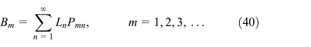
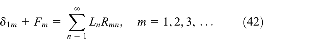
Although we can solve equations (40)–(55) for unknown coefficients, we prefer coupling the above systems of equations for the sake of convenience. From equations (40) and (51), we have

\sum_{n = 1}^{\infty} L_{n} P_{mn} ({\hat{μ}}_{m} + {\hat{λ}}_{n}) = 0, m = 1, 2, 3, \dots

(56)

whereas equations (41) and (52) yield

\sum_{n = 1}^{\infty} L_{n} Q_{mn} ({\hat{α}}_{m} + {\hat{λ}}_{n}) = 0, m = 1, 2, 3, \dots

(57)

From equations (42) and (53), we have

\sum_{n = 1}^{\infty} L_{n} R_{mn} ({\hat{β}}_{m} + {\hat{λ}}_{n}) = ({\hat{β}}_{1} + {\hat{β}}_{m}) δ_{1 m}, m = 1, 2, 3, \dots

(58)

equations (43) and (54) give

\sum_{n = 1}^{\infty} L_{n} S_{mn} ({\hat{α}}_{m} + {\hat{λ}}_{n}) = 0, m = 1, 2, 3, \dots

(59)

From equations (44) and (55), we have

\sum_{n = 1}^{\infty} L_{n} T_{mn} ({\hat{μ}}_{m} + {\hat{λ}}_{n}) = 0, m = 1, 2, 3, \dots

(60)

Convergence

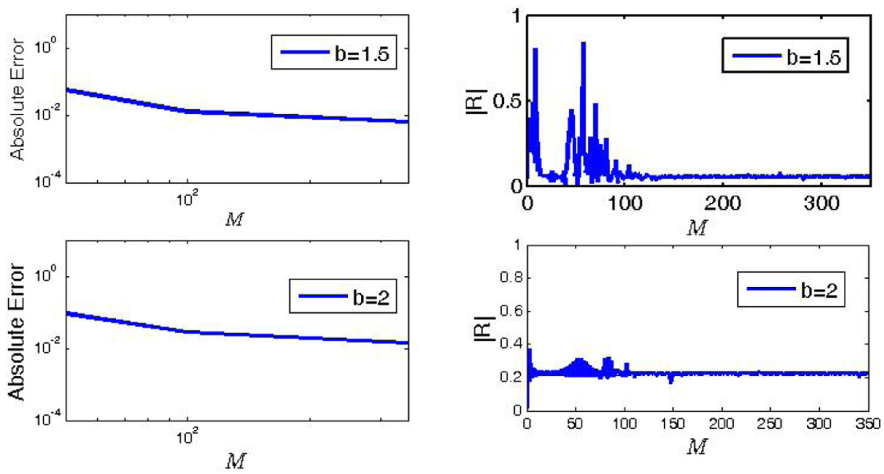
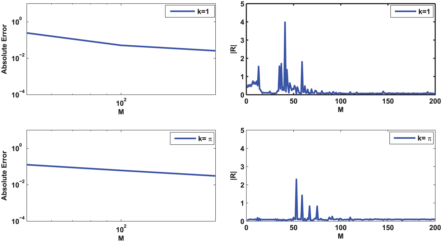
In Figure 2, we present the reflected field amplitude against the truncation number M for various dimensions of the pentafurcated duct. Figure 2 depicts that the graph becomes insensitive for $M > 150$ when we choose $a = 1$ , $b = 1.5$ , $d = 3$ , and $k = π$ . We also present graphically the absolute error value of the reflection coefficient R on log scale versus the truncation number M for same dimensions in this figure by using the Richardson extrapolation formula. Similarly, Figure 3 is drawn to show the convergence of our results for different duct spacing such that $a = 1, b = 2, d = 3$ , and the wave number $k = 1$ and $k = π$ . Similarly, we plot Figure 4 for $a = 1, b = 2$ , and $d = 4$ , while k has values 0.5 and 1. In both Figures 3 and 4, we observe that the values of the reflection becomes insensitive for $M > 100$ . The infinite systems of equations converges relatively slowly so we can truncate at $M \approx 170$ in our calculations, which gives us errors to line width. The convergence will hit the computer limit eventually.

Figure 2.

Reflected field amplitude |R| versus the truncation number M for $a = 0.5$ , $d = 3$ , and $k = π$ .

Figure 3.

Reflected field amplitude |R| versus the truncation number M for $a = 1$ , $b = 2$ , and $d = 3$ .

Figure 4.

Reflected field amplitude |R| versus the truncation number M for $a = 1$ , $b = 2$ , and $d = 4$ .

Numerical results

Now, we solve $L_{n}$ from infinite systems of equations (56)–(60) by taking $n = 1, 2, 3, \dots, 5 M$ and $m = 1, 2, 3, \dots, M$ . Then, we determine the other amplitudes in different regions from equations (40)–(44). We consider the incident mode $e^{i \hat{β_{1}} x}$ having amplitude 1 to find out the intensity of the acoustic wave of the given geometry. The fundamental mode in region III corresponds to $n = 1$ and $| R | = | F_{1} |$ represents the reflection coefficient of $e^{- i \hat{β_{1}} x}$ . The radiated power is represented by $(1 - | R |^{2})$ which comes out from semi-infinite region III of pentafurcated duct. The absolute value of the reflected field amplitude |R| determines the energy of the incident mode which is distributed among the other regions of the duct. We depict the graphical representation of the reflected field |R| against the wave number k for various dimensions of the duct. The comparison of the reflected field amplitude |R| for the given problem and the hard duct problem¹⁹ is also presented.

Case 1

In this case, the dimension of the duct is such that no wave propagates in regions I, II, IV, and V. Then, consequently, two modes propagate in region VI; Figure 5 represents this situation graphically. In Figure 5, we present the absolute value of the reflection coefficient against the wave number k with duct dimensions $a = 1$ , $b = 1.5$ , and $d = 2.5$ over the frequency range $0 < k < 3 π / 4$ . In Figure 5, the values of the non-dimensional wave number $k = π / 10, π / 4, 3 π / 10$ , and $π / 2$ correspond to the cut-on frequencies of regions VI, III, VI, and I, respectively. We show them as vertical dotted lines.

Figure 5.

Reflected field amplitude |R| versus the wave number k for $a = 1$ , $b = 1.5$ , and $d = 2.5$ .

Case 2

In case (2), we consider only one wave that propagates in each of the region $(- d < y < d, x < 0)$ . Consequently, five waves propagate toward the forward direction in region VI. Figure 6, shows |R| versus the wave number for the case $(2)$ , with duct spacing at $a = 1$ , $b = 2$ , and $d = 3$ and the frequency range $0 < k < 15 π / 12$ . We can see from Figure 6 that the radiated energy will be increased for excitation of higher order modes in region III or VI since the reflected field amplitude decreases. $k = π / 4$ is the cut-on frequency of region III or VI. The vertical lines in Figure 6, correspond to cut-on(off) frequencies in different regions.

Figure 6.

Reflected field amplitude |R| versus the wave number k where $a = 1$ , $b = 2$ , and $d = 3$ .

Case 3

Figure 7 depicts the graph of |R| against k with frequency range $π / 4 < k < 3 π / 4$ . In this case, the duct spacing $b = 2$ and $d = 3$ is fixed while the duct spacing “a” has the 0.5 and 1. In Figure 7, the solid and chained lines are for $a = 1$ and $a = 0.5$ , respectively.

Figure 7.

Reflected field amplitude |R| versus the wave number k for $b = 2$ and $d = 3$ .

Case 4

Here, we consider the dimensions of the pentafurcated duct such that “b” has two different values 2 and 1.5, while $a = 1$ and $d = 3$ are fixed. Figure 8 is plotted for this case with frequency range $π / 4 < k < 3 π / 4$ . Figure 9 is plotted when the values of d changes from 3 to 4 for $a = 1$ and $b = 2$ are fixed. The frequency range is $π / 4 < k < 3 π / 4$ .

Figure 8.

Reflected field amplitude |R| versus the wave number k for $a = 1$ and $d = 3$ .

Figure 9.

Reflected field amplitude |R| versus the wave number k for $a = 1$ and $b = 2$ .

Comparison

In Figure 10, we plot the reflection coefficient |R| for the hard duct (dashed lines) and for the current waveguide problem (solid lines) over the same frequency range $(0 < k < 3 π / 4)$ . The dimensions of the ducts for both problems are such that $a = 1$ , $b = 1.5$ , and $d = 2.5$ . The power transmission for both the ducts is proportional to $(1 - | R |^{2})$ for the given fundamental mode. The acoustic energy exiting from the mixed soft–hard (current problem) is smaller than the hard duct problem,¹⁹ in the frequency range $0.8 < k < 1$ and $1.26 < k < 3 π / 4$ . We observe that the reflection coefficient decreases monotonically from the cut-on(off) frequency $π / 2$ in the case of soft–hard duct for onward frequencies. In case of hard duct, the reflection coefficient for the fundamental mode decreases more slowly when we increase the frequency range from cut-on(off) frequency $2 π / 5$ . Similarly, Figure 11 depicts the comparison between the current problem and the hard pentafurcated problem for $a = 1, b = 2$ , and $d = 3$ . The frequency range is $0 < k < 4$ . We have noticed that the sum of the values of reflection coefficient is smaller than the sum of the values of reflection coefficient for hard pentafurcated duct for the given dimensions in Figures 10 and 11, thus radiating less energy to other regions. Hence, soft lining improves the performance of the hard boundary pentafurcated duct.

Figure 10.

Reflected field amplitude |R| versus the wave number k where $a = 1$ , $b = 1.5$ , and $d = 2.5$ .

Figure 11.

Reflected field amplitude |R| versus the wave number k for $a = 1$ , $b = 2$ , and $d = 3$ .

Energy conservation

We now use Green’s identity

\begin{matrix} \int \int_{D} ((\nabla^{2} v + k^{2} v) v^{*} - (\nabla^{2} v^{*} + k^{2} v^{*}) v) d s \\ = \oint_{\partial D} (v^{*} \frac{\partial v}{\partial x} - v \frac{\partial v^{*}}{\partial x}) d y = 0 \end{matrix}

(61)

to define the energy conservation relationship of the incident, reflected, and transmitted waves. In our problem, $v (x, y)$ is the solution of equation (5) which satisfies boundary conditions (6)–(11). Where * represents the conjugate and D is the region of the duct $(- d < y < d, - \infty < x < \infty)$ having cuts for the semi-infinite ducts. We consider one wave that propagates in each of the five regions I–V $(| y | < d, x < 0)$ . Then, it is not difficult to define energy conservation relationship (62) from equation (61).

\begin{matrix} \hat{β_{1}} (1 - {| F_{1} |}^{2}) = \hat{μ_{1}} {| B_{1} |}^{2} + \hat{α_{1}} {| D_{1} |}^{2} + \hat{α_{1}} {| H_{1} |}^{2} \\ + \hat{μ_{1}} {| J_{1} |}^{2} + \sum_{j = 1}^{5} \hat{λ_{j}} {| L_{1} |}^{2}, \end{matrix}

(62)

where $\hat{β_{1}} (1 - {| F_{1} |}^{2})$ indicates the radiated power that belongs to the middle region $(- a < y < a, x < 0)$ which is divided among the other regions. To validate the analytical mode-matching approach, we calculate the energy balance relation (62) for few values of wave number k. We have noticed for the configuration of Figure 6 that the acoustic radiated power in region III (LHS of equation (62)) at $k = π / 4$ is 0 which is equal to the acoustic transmitted power (RHS of equation (62)). This shows that the reflection is $- 1$ and no energy is transmitted among the other regions. Also, at $k = π / 2$ , the difference in the acoustic radiated power $(1.3499)$ and the transmitted power $(1.3490)$ is $8.3488 \times 10^{- 4}$ . This may be due to the contribution of the remaining decaying modes.

Summary

The pentafurcated design problem has been investigated which consists of soft–hard boundaries. The mode-matching technique has been applied when the fundamental mode is assumed to propagate in the middle region $(| y | < a, x < 0)$ of the pentafurcated duct since it has an important role in practical applications. Numerically, the field amplitudes are determined for different dimensions of the pentafurcated duct. In Figure 5, the cut-on(off) frequencies are at $k = π / 4, 3 π / 10$ , and $π / 2$ . In Figure 5, no wave propagates in any of the coaxial regions $(- d < y < - b, - b < y < - a, - a < y < a, a < y < b$ , and $b < y < d)$ for $x < 0$ . We can see more abrupt changes in graph (6) when one wave propagates in each of the region $(| y | < d, x < 0)$ . The cut-on(off) frequencies are at $k = π / 12, π / 4, 5 π / 12, π / 2, 7 π / 12, 3 π / 4, 11 π / 12$ , and $13 π / 12$ . In this situation, five waves travel in the forward direction and four waves travel in the backward direction. Figures 7 –9 are presented when one of the duct spacing varies, while the other two duct spacing are fixed. We observed that the values of the reflection decreases as the dimensions of the duct spacing “a” increases. In Figures 5 –9, we have noticed that the reflected field coefficient is 1 at certain cut-on(off) frequencies of the different regions. This corresponds to signify minimum transmission downstream or possibly, the maximum attenuation produced. We have carried out the convergence of the reflected field |R| against the truncation number M to demonstrate the accuracy of the presented work. At the end, to compare our results with the existing hard pentafurcated problem,¹⁹ we plotted the reflected field amplitude versus the wave number k for soft–hard pentafurcated and the hard pentafurcated. We observe that soft surface does have more noise-reducing effect than the hard surface. It is probable that in the given problem, soft linings provide an upper bound for attenuating noise effect which is produced by soft absorbent lining as compared to hard duct. The Wiener–Hopf technique requires the geometry of configuration to be infinite or semi-infinite. The analytical mode-matching technique allows one to consider the finite length chamber. So, we will try to tackle such problem in future work. This research work will be helpful for engineers and physicists to form new devices or exhaust systems to attenuate noise effect.

Footnotes

Academic Editor: Francisco Denia

Declaration of conflicting interests

The author(s) declared no potential conflicts of interest with respect to the research, authorship, and/or publication of this article.

Funding

The author(s) received no financial support for the research, authorship, and/or publication of this article.

References

Andronov

Belinsky

B P.

On acoustic boundary-contact problems for a vertically stratifed medium bounded from above by a plate with concentrated inhomogenties. Prikl Maten Mekhan 1990; 54: 366–371.

Lawrie

Abrahams

ID.

An orthogonality condition for a class of problems with high order boundary conditions, application in sound/structure interaction. Q J Mech Appl Math 1999; 52: 161–181.

Lawrie

Kirby

Mode-matching without root-finding: application to a dissipative silencer. J Acoust Soc Am 2006; 119: 2050–2061.

Lawrie

JB.

On eigenfunction expansions associated with wave propagation along ducts with wave bearing boundaries. J Appl Math 2007; 72: 376–394.

Lawrie

JB.

Analytic mode-matching for acoustic scattering in three dimensional waveguides with flexible walls, application to a triangular duct. Wave Motion 2013; 50: 542–557.

Ammari

Kang

Santosa

Scattering of electromagnetic waves by thin dielectric planar structures. SIAM J Appl Math 2006; 38: 1329–1342.

Ammari

Bretin

Garnier

. Noise source location in an attenuating medium. SIAM J Appl Math 2012; 72: 317–336.

Nawaz

Ayub

Closed form solution of electromagnetic wave diffraction problem in a homogeneous bi-isotropic medium. Math Method Appl Sci 2015; 38: 176–187.

Nawaz

Afzal

Ayub

Acoustic propagation in two-dimensional waveguide for membrane bounded ducts. Commun Nonlinear Sci Numer Simul 2015; 20: 421–433.

10.

Buyukaksoy

Tayyar

Uzgoren

Influence of the junction of perfectly conducting and impedance parallel plate semi-infinite waveguides to the dominant mode propagation. J Math Anal Appl 2006; 143: 341–357.

11.

Buyukaksoy

Cinar

Serbest

Scattering of plane waves by a junction of a transmission and soft/hard half-planes. J Appl Math Phys (ZAMP) 2004; 55: 483–499.

12.

Buyukaksoy

Cinar

Solution of a matrix Wiener-Hopf equation connected with the plane wave diffraction by an impedance loaded parallel plate waveguide. Math Method Appl Sci 2005; 28: 1633–1645.

13.

Rawlins

AD.

A bifurcated waveguide problem. J Appl Math 1995; 54: 59–81.

14.

Hassan

Rawlins

AD.

Sound radiation in a planar trifurcated lined duct. Wave Motion 1999; 29: 157–174.

15.

Ayub

Tiwana

Zaman

Acoustic wave propagation in a trifurcated lined waveguide. ISRN Appl Math 2011; 2011: 1–19.

16.

Ayub

Tiwana

Mann

AB.

Wiener-Hopf analysis of an acoustic plane wave in a trifurcated waveguide. Arch Appl Mech 2011; 81: 701–713.

17.

Ayub

Tiwana

Mann

AB.

Influence of the acoustic dominant mode propagation in a trifurcated lined duct with different impedance. Phys Scr 2010; 81: 035402.

18.

Hassan

MU.

Wave scattering by soft–hard three spaced waveguide. Appl Math Model 2014; 38: 4528–4537.

19.

Hassan

Meylan

Bashir

. Mode matching analysis for wave scattering in triple and pentafurcated spaced ducts. Math Method Appl Sci 2016; 39: 3159–3530.

20.

Mei

(ed.). The applied dynamics of ocean surface waves. New York: John Wiley & Sons, 1983.

21.

Linton

Mclver

(eds). Handbook of mathematical techniques for wave/structure interactions. New York: Chapman & Hall/CRC Press, 2001.

Reflected field analysis of soft–hard pentafurcated waveguide

Abstract

Keywords

Introduction

Formulation of pentafurcated waveguide problem

Region I { − d ≤ y ≤ − b , x < 0 }

Region II { − b ≤ y ≤ − a , x < 0 }

Region III { − a ≤ y ≤ a , x < 0 }

Region IV { a ≤ y ≤ b , x < 0 }

Region V { b ≤ y ≤ d , x < 0 }

Region VI { − d ≤ y ≤ d , x > 0 }

Solution of the pentafurcated waveguide problem

Continuity of pressure

Continuity of velocity

Coupling

Convergence

Numerical results

Case 1

Case 2

Case 3

Case 4

Comparison

Energy conservation

Summary

Footnotes

Declaration of conflicting interests

Funding

References

Region I ${- d \leq y \leq - b, x < 0}$

Region II ${- b$ $\leq y$ $\leq - a, x < 0}$

Region III ${- a$ $\leq y$ $\leq a, x < 0}$

Region IV ${a$ $\leq y$ $\leq b, x < 0}$

Region V ${b$ $\leq y$ $\leq d, x < 0}$

Region VI ${- d$ $\leq y$ $\leq d, x > 0}$