Sage Journals: Discover world-class research

Abstract

Although vortex flowmeters are widely used in various industries, the accuracy of vortex flowmeter measurements depends on inlet flow conditions. In this study, flow fields of a vortex flowmeter with various inflow conditions are simulated numerically. In order to model transient turbulent flows, Large Eddy Simulation and vortex shedding frequencies are determined using fast Fourier transform techniques. To determine the frequency characteristics in the area of downstream of the vortex generator, both steady and unsteady velocity profiles are used as inlet conditions, including two different shear flows and various sinusoidal plug flows. For steady inlet conditions, the flow qualities along the pipe are quantified using a proposed definition to express a velocity profile which departs from a fully developed velocity profile. For unsteady inlet conditions, the predominant frequency pattern is successfully predicted and it is linked to the measurement accuracy of the vortex flowmeter.

Keywords

Vortex flowmeter inflow conditions vortex shedding frequency

Introduction

Vortex flowmeters¹ are widely used in various industries because of their high accuracy, wide measurement range, excellent linearity, resistance to corrosion, and low cost in terms of investment and maintenance. However, the drawbacks of vortex flowmeters are flow disturbances and fluid turbulence in practical applications. Therefore, vortex flowmeters are more sensitive to installation parameters as compared with other flowmeters. Specific requirements ensure accurate flow rates when measurements are taken downstream of valves, diverters, elbows, or converging pipes which may induce considerably flow disturbances.^2,3 However, many flowmeters are still improperly installed because of spatial limitations or other practical constraints.^4,5 Tests were performed using flow calibration equipment in the laboratory of Energy Management System Co., Ltd, which has an ISO 17025 accreditation.^6,7 The experimental results showed that some upstream pipeline configurations can produce unacceptable measurement errors in the vortex-type flowmeter, and the measurement accuracy of the vortex flowmeter depends on the qualities of the incoming flows more than other types. Therefore, in order to achieve accurate measurements of a vortex flowmeter, adverse effects such as poor inflow conditions caused by improper installation must be studied and understood.

It is impractical to develop a set of general criteria for quantifying the effectiveness of a vortex flowmeter installation due to the various meter-dependent measuring characteristics which could only be verified by performing extensive experiments. Many experiments have been carried out to study the effects of installed flowmeters in the past decade.^8,9 For example, wind tunnel experiments have been used to produce uniform upstream flows to study flow fields. In reality, however, most upstream flow fields are three-dimensional (3D) and non-uniform. Miau et al.¹⁰ studied the uncertainties in vortex flowmeter measurements and found that the accuracy of flowmeters is significantly affected by upstream flow conditions in a 3D non-uniform flow field. Hsiao and Chiang¹¹ found two to three constant-frequency vortex cells in the shedding vortices generated along the spanwise direction of a tapered circular cylinder. The above-mentioned studies suggest that the vortex shedding characteristics of a bluff body are substantially affected by upstream flow conditions.¹²

Numerical simulations in engineering applications are becoming very popular in various industries because of rapid progresses of computer software and hardware. Computational fluid dynamics (CFD) analyses are widely used to predict the flow fields for engineering design features and to extrapolate experimental limitations. The SIMPLE algorithm developed by Patankar¹³ for solving incompressible flow was used in this study.¹⁴ A CFD code is useful only when the predictions of a set of parameters of a certain flow field are validated by experiments. In order to generate a turbulent wake for vortex flowmeter measurements, a turbulent flow with a Reynolds number higher than 300 is required.¹⁵ Therefore, turbulent flow must be modeled in numerical simulations of vortex flowmeters for a flow with a high Reynolds number in present applications.

ANSYS FLUENT CFD code is used in this study to solve the turbulent flow field when a vortex flowmeter is installed in a pipe with different inflow conditions. This study analyzed several inflow conditions at the entrance of the pipe including a fully developed flow, two shear flows, and various sinusoidal plug flows. The effects of various inlet flow conditions on the predominant frequency shift, which affect the accuracy of the vortex flowmeter, are also determined. In this article, governing equations and boundary and initial conditions are described in section “Theoretical methods. Numerical treatments for simulation are provided in section “Numerical simulations” with verification by grid independent tests and validation with experiments. Numerical results and discussion are stated in section “Results and discussion” and conclusions are summarized in section “Concluding remarks.”

Theoretical methods

The CFD simulation is simplified as a transient incompressible turbulent flow with no heat generation. No-slip boundary conditions are used on the walls of the pipe and the vortex generator.

Governing equations

A general transport equation, in conservation form, for mass and momentum in the 3D Cartesian coordinate system is described as follows^13,16

\begin{array}{l} \frac{\partial (ρ ϕ)}{\partial t} + \frac{\partial (ρ ϕ u)}{\partial x} + \frac{\partial (ρ ϕ v)}{\partial y} + \frac{\partial (ρ ϕ w)}{\partial z} \\ = \frac{\partial}{\partial x} (Γ \frac{\partial ϕ}{\partial x}) + \frac{\partial}{\partial y} (Γ \frac{\partial ϕ}{\partial y}) + \frac{\partial}{\partial z} (Γ \frac{\partial ϕ}{\partial z}) + S \end{array}

(1)

where S is the source term of the pressure gradient and the gravitational force and $Γ$ is the diffusion coefficient. The first term shows the transient characteristic of this problem. The symbol $ϕ$ can be replaced by 1 for the continuity equation, and u, v, and w are the momentum equations in the X-, Y-, and Z-directions, respectively. Since the fluid used in this study is water, the density is assumed to be constant in the flow field. Equation (1) can be expressed in generalized coordinates using the finite volume method for numerical simulation. This study uses Large Eddy Simulation (LES), which is one of the computational tools for studying turbulent flow fields.^17–19

The inlet flow conditions described below are used to determine the effect of inflow conditions on the measurement accuracy of a vortex flowmeter, and they are specified at half of the pipe diameter upstream of the vortex generator. In this article, a one-seventh power-law velocity profile as expressed in equation (2) is used to simulate a standard fully developed turbulent flow in a sufficiently long pipe¹⁸

V = V_{c} {[1 - \frac{r}{R}]}^{\frac{1}{n}}, 0 \leq r \leq R

(2)

where n is a velocity profile index which depends on the Reynolds number, $V_{c}$ is the velocity along the pipe center line, r is the radial coordinate and R is the radius of the pipe. In this study, the values, V_c = 4.244 m/s, n = 7, and R = 0.075 m, have been given to make sure the inlet volume flow rate (0.0636 m³/s) is conserved for the uniform velocity ( $\bar{V} = 3.6 m / s$ ), the power-law velocity of equation (2) and the experimental data.

A distorted flow caused by a specific upstream piping configuration is simulated using equation (3) to express a shear velocity profile varying in the spanwise direction at the inlet

V = V_{c} + V_{c} [\frac{r}{R}], - R \leq y \leq R

(3)

where shear flow conditions are analyzed with the upstream velocity (x-direction) varying in a spanwise direction (y-direction), or in a transverse direction (z-direction), with respect to the vortex generator.

In addition to the disturbance caused by the piping configuration, unsteady plug flows with a sinusoidal axial velocity variation are simulated using the equation

V = V_{c} + ε V_{c} [\sin (ω t)]

(4)

where ω indicates the exciting angular frequency (2πf), ε is the amplitude of the fluctuation, and t is the time for the transient simulation. Equation (4) derives the time-varying inflow velocity distribution by manipulating the exciting frequency and the amplitude of the sinusoidal fluctuation. In this study, $V_{c}$ is a constant value and equation (4) represents sinusoidal plug flows.

In experimental measurements, the predominant vortex shedding frequency is determined by the load signals from a pressure sensor located downstream of the vortex generator. The proposed numerical method acquired the waveform of total lift coefficient ( $C l = L / (0.5 ρ V^{2} A)$ ; L is lift) by directly integrating the surface of the vortex generator over a time period. A fast Fourier transform (FFT) technique is then used to compute the power spectral density of the lift-coefficient variation and the predominant frequency can be determined for analysis.

Determination of flow qualities

Pipe fittings located upstream of the flowmeter inevitably cause distortion of the flow field, and accordingly affect the measurement accuracy of the flowmeter. To quantify the distortion in the upstream flow field, this study uses a method developed by Miau et al.²⁰ Therefore, the numerical form for the departure from the axial velocity profile over a cross-sectional plane of the pipe can be written as

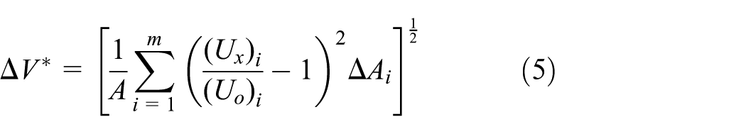
Δ V^{*} = {[\frac{1}{A} \sum_{i = 1}^{m} {(\frac{{(U_{x})}_{i}}{{(U_{o})}_{i}} - 1)}^{2} Δ A_{i}]}^{\frac{1}{2}}

(5)

where i denotes the grid index in the radial direction, m is the total grid number, A is the cross-sectional area of the pipe, $Δ A_{i}$ is the area of the ith grid, ${(U_{x})}_{i}$ denotes the mean axial velocity at grid i, and ${(U_{o})}_{i}$ is the mean axial velocity based on a fully developed flow. According to this definition, the term, $Δ V^{*}$ , expresses the velocity-profile departure from a fully developed flow. Thus, $Δ V^{*}$ represents the degree of velocity distortion at a specific location as compared with a fully developed flow at a specific Reynolds number. In this study, $Δ V^{*}$ is used to determine the departure from the fully developed flow for steady shear flows.

Numerical simulations

To determine the relationship between flow inlet and shedding vortex, the signal generated by the vortex generator is numerically analyzed to obtain the frequency characteristics of the vortex meter.

Validations of the computer code

In addition to this simulation methodology validated by reproducing canonical Karman vortex shedding behind a circular cylinder, a commercially available VK150 vortex flowmeter is used for numerical validation. This flowmeter has an inner diameter of 150 mm and an internal trapezoidal cylinder with a characteristic width of 42 mm as shown in Figure 1. To achieve reasonable boundary conditions far upstream and downstream in simulations of the flowmeter, the computational domain is established by connecting a hollow pipe at both ends of the flowmeter. Figure 2, which is the solid model obtained by computer-aided design (CAD) software, shows that the lengths of added pipes are 0.5 times the diameter at the front end of the flowmeter and 1.5 times the diameter at the rear end. For clarity, Figure 2 shows the Cartesian coordinate set at the inlet of the flowmeter, where the origin of the coordinates is located at the center of the pipe. The X-axis is the direction of the axial flow along the pipe, the Y-axis is the spanwise direction of the vortex generator, and the Z-axis is the transverse direction with respect to the vortex generator.

Figure 1.

Commercial vortex meter (VK150; Energy Management System Co., Ltd) used in the experiments.

Figure 2.

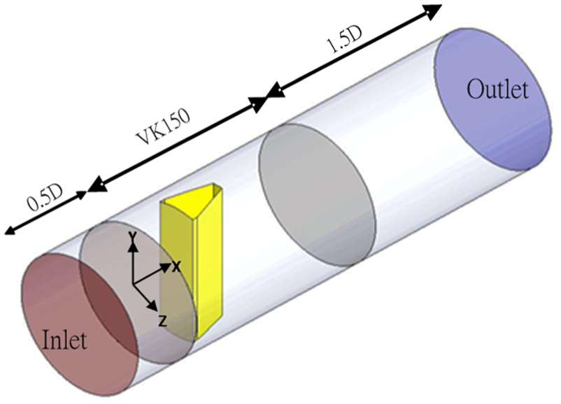
Coordinate system for the computational domain.

For a standard case in this study, the inlet flow is assumed to be fully developed as shown in equation (2). The value of V_c in equation (2) is determined using a mass flow rate with an average velocity of 3.6 m/s, which is the typical operational velocity for the considered vortex flowmeter and is equivalent to a Reynolds number of $5.38 \times 10^{5}$ . The Reynolds number is defined as Re = ρVD/µ, where ρ is the density of the fluid, V is the average flow velocity, D is the inner diameter of the pipe, and µ is the dynamic viscosity of the fluid. The outflow boundary condition is set for zero-order extrapolation of the related flow properties. No-slip condition is applied to all surfaces, including those of the inner pipe wall and the vortex generator. The following numerical techniques are then used to obtain stable and accurate solutions:

The vortices generated from a two-dimensional (2D) circular cylinder become turbulent when Reynolds number exceeds 300.^15,21 Therefore, the standard k–ε turbulence model is provided to approximate the Reynolds stresses without time evolution. The obtained data are then imported to the solver for LES as the initial conditions for transient calculations. This procedure is found to yield rather stable calculation results. According to the literature, LES has a great potential for calculating these complex flows.¹⁹ In this study, LES is activated at the beginning of calculation when the time evolution for vortex formation is studied. Smagorinsky–Lilly model is used for subgrid model in LES and the Smagorinsky constant is set to be 0.1. At the inlet boundary, turbulence intensity is estimated based on the Reynolds number and expressed as I = 0.16 Re^−1/8.¹⁸

In order to effectively compute the present flow fields, the flow domain is divided into smaller subdomains. Structured hexahedral grids are adopted to build the mesh surrounding the vortex generator. Around the generator, mixed grid types are used to fit the space inside the pipe. Additionally, finer grids are imposed along the boundary wall to resolve the turbulent boundary layer and the grid scale relative to viscous scale is calculated to be of approximately two orders of magnitude. Figure 3 shows the calculations for the grid independence check. The non-dimensional frequencies, f*/f, from different grid systems approach to 1, where f* is the experimental value for comparison and f is acquired by doing FFT for the evolution of Cl over the elapsed time. The calculations show that 0.95 million grids are suitable for the study.

When ANSYS FLUENT solves the time-dependent equations using an implicit formulation, multiple iterations may be necessary at each time step. Users have to set a maximum parameter for the number of iterations per time step. If the convergence criteria are met before this number of iterations is performed, the solution will advance to the next time step. The maximum parameter for the number of iterations per time step must be carefully specified to avoid error propagation in the calculations. A globally scaled residual of $5 \times 10^{- 4}$ is used to check the absolute convergence criteria for each time step.¹⁶

Time step for the calculation must be sufficiently small for an adequate resolution in the time domain and for an accurate determination of the predominant frequency by a FFT algorithm. In this study, the time step is set to be 0.001 s and the time-step scale relative to the small-eddy time scale is calculated to be of approximately two orders of magnitude. The Cl plot of 4000 points is performed by the FFT to obtain frequency spectra for each case. Figure 4 shows the numerical results obtained from the implicit time integration method by comparing with the experiment with a time step of 0.001 s. A typical frequency for vortex shedding in present cases is approximately 20 Hz so that a time period is set to be approximately 0.05 s. Therefore, 50 calculation steps are needed to resolve a single complete cycle of vortex shedding.

The time history of the induced lift is used in the FFT to obtain a predominant frequency for vortex shedding. If conventional FFT is used to evaluate the spectrum for a data string with a non-sinusoidal part, the resulting spectrum has an exponentially decaying envelope. The data for the low-frequency part are highly contaminated. Similarly, the non-periodic condition often yields an adverse contribution. Therefore, an iterative filter proposed by Jeng et al.²² is used to remove the non-sinusoidal trend and reduce the error induced by the non-periodic condition.

Figure 3.

Grid independence check for the study.

Figure 4.

Comparisons of numerical and experimental results for the standard case.

Comparisons between the numerical and experimental data for the standard case are shown in Figure 4. The standard case uses a fully developed velocity profile as the inlet condition and is denoted as Case A. The Strouhal number is defined as St = fd/V, where f is the predominant vortex shedding frequency and d is the width of the front face of the vortex generator. The experiment is performed in a laboratory with an ISO 17025 accreditation by Taiwan Accreditation Foundation.⁷ The machine error for the experiment is within 2% (error bars in Figure 4). The error bars on the CFD results to show the deviations between the fitted curve and individual calculated points are also included in Figure 4 (maximal relative error, ∼5%). Generally, the numerical and the experimental values for the Strouhal numbers are consistent for the range of Reynolds numbers. Figure 5 shows the animated frames of the coherent structure of vortex shedding in a time period, T, on the central plane, that is, the X-Z plane at Y = 0, for this standard case. Figure 6(a) shows the sketch of the inlet flow for the benchmark Case A, which is used to derive a suitable grid distribution and number for the remaining numerical experiments.

Figure 5.

Animated frames of the coherent structure of the vortex shedding in a time period on the middle plane of the pipe, for Case A, where average velocity V = 3.6 m/s.

Figure 6.

Inflow conditions for numerical simulation. (a) Case A: fully developed flow, (b) five regions along the generator, (c) Case B1: shear flows in the Y-axis, and (d) Case B2: shear flows in the Z-axis.

Numerical experiments

The standard case was used as a reference in several comparisons of the effect of upstream flow conditions on vortex shedding for the vortex flowmeter. Figure 6(b) shows how local vortex shedding frequencies are resolved by dividing the integration domain into five equal regions over the vortex generator surface. The highest and lowest regions are denoted as regions 1–5, respectively, where gravity acts in the negative Y-axis direction. Figure 6(c), Case B1, represents the shear flow in the spanwise direction, that is, the Y-axis direction, of the vortex generator, and Figure 6(d) (Case B2) represents the shear flow in the transverse direction, that is, the Z-axis direction.

Sinusoidal plug flows, that is, $V = V_{c} + ε V_{c} [\sin (ω t)]$ , with fluctuating frequencies and amplitudes at the same flow rate, are used to determine the effect of streamwise inlet velocity. Case C is a steady plug flow with an average velocity inlet, ε = 0 and V = 3.6 m/s. Cases C1, C1, and D show the effect of various velocity amplitudes as compared with Case C. Case D is chosen as a reference case, with ω = 2πf = 140 and ε = 0.5, which is equivalent to a frequency of 22 Hz. Cases D1–D5 represent the similar sinusoidal plug flows with the same amplitude of velocity fluctuation under different frequencies. Table 1 summarizes the details for all plug flows.

Table 1.

Summary of the inlet flow features.

Case	Inlet velocity	Comment
C	$V = V_{c}$	Steady plug flow at inlet
C1	$V = V_{c} + 0.1 V_{c} [\sin (140 t)]$	Comparisons with Case D, for various exciting amplitudes^a
C2	$V = V_{c} + 0.2 V_{c} [\sin (140 t)]$	Comparisons with Case D, for various exciting amplitudes^a
D	$V = V_{c} + 0.5 V_{c} [\sin (140 t)]$	Unsteady plug flow at inlet^a
D1	$V = V_{c} + 0.5 V_{c} [\sin (35 t)]$	Comparisons with Case D, for various exciting angular frequencies
D2	$V = V_{c} + 0.5 V_{c} [\sin (70 t)]$
D3	$V = V_{c} + 0.5 V_{c} [\sin (137.5 t)]$
D4	$V = V_{c} + 0.5 V_{c} [\sin (210 t)]$
D5	$V = V_{c} + 0.5 V_{c} [\sin (280 t)]$

The value of ω = 140 for the standard case D is equivalent to the shedding frequency of 22.29 Hz.

Results and discussion

Single-precision calculations are performed with ANSYS FLUENT in two networked desktop computers. In each computer, a four-core CPU runs the parallel calculations by sharing memory allocations on the local machine. Nevertheless, the hardware still requires approximately 1.5 days because simulating unsteady turbulent flow is very time-consuming.

Shear flow at inlet

Since the Strouhal number for vortex shedding is invariant for a uniform flow passing through a 2D cylinder, this study investigates whether shedding frequencies vary along the vortex generator for the upstream shear flow conditions, that is, Cases B1 and B2. Table 2 shows the local predominant vortex shedding frequency for Case A in each region for a fully developed upstream velocity. Each region has the same reference frequency of 22.1 Hz, which is the value in the central region in Case A, but regions 4 and 5 have minor deviations. Visualizing the flow animation on the test plane in each corresponding region shows that the vortex flow structures are very similar. Therefore, when the upstream flow is fully developed, the circular boundary of the pipe wall does not substantially affect the local vortex shedding frequency along the spanwise direction of a vortex generator with a constant cross section. It is postulated that these minor deviations in the lower portion of the tube result from the combined effects of the circular wall, gravitational force, and numerical errors. Figure 7 shows the time histories for the lift coefficients across the surface of a vortex generator in regions 1, 3, and 5, for Case A. In each region, the shedding frequency is very similar, and phase lag is minimal. Figure 7(a) clearly shows that oscillation occurs at 0.1 s and stabilizes at 4.0 s as shown in Figure 7(b).

Table 2.

Predominant frequencies (Hz) for vortex shedding in steady input velocity profiles.

Region	Case
	A	B1		B2
	Reference frequency	Shedding frequency	Deviation (%)	Shedding frequency	Deviation (%)
Region 1	22.1	23.4	5.88	22	−0.45
Region 2	22.1	23.3	5.43	22.5	1.81
Region 3	22.1	23.4	5.88	22.5	1.81
Region 4	21.9	23.3	5.43	22.6	2.26
Region 5	22.5	20.1	−9.05	22	−0.45

Figure 7.

Lift coefficients in different regions in Case A: (a) t = 0–0.16 s and (b) t = 3.9–4 s.

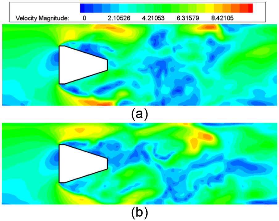
For a shear flow at inlet, Cases B1 and B2 simulate flows that are distorted by upstream piping configurations. For the shear flow in the Y-axis, Case B1, the velocities generated form the vortex generator vary substantially at the two ends. Velocity is highest in region 1 and lowest in region 5. Since the Reynolds number differs in each region, the axis of the shed vortex inclining relative to the vortex generator is expected.²³ Table 2 shows that the shedding frequencies in regions 1–4 (23.3–23.4 Hz) are higher than that in region 5 (20.1 Hz). Figure 8 shows the velocity contours for Case B1 on the central planes for regions 1 and 5 at 0.5 time period. The velocities in region 1 are lower at downstream of the vortex generator, but the velocities in region 5 are comparatively higher. This indicates that momentum changes cause flow mixing in the Y-axis from upstream to downstream. Figure 9 shows the time histories for the lift coefficients on the surface of the vortex generator in regions 1, 3, and 5, for Case B1. The shedding frequencies in regions 1 and 3 are very similar, and the phase difference does not significantly differ by regions. However, the Cl waveform in region 5 lags behind the Cl waveform in region 1 or 3 by some phase angle.

Figure 8.

Velocity contours for Case B1 at 4/8T on the central planes of regions 1 and 5: (a) region 1 and (b) region 5.

Figure 9.

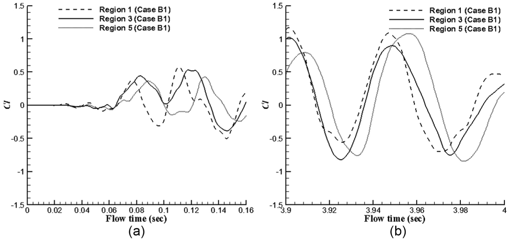
Lift coefficients in different regions in Case B1: (a) t = 0–0.16 s and (b) t = 3.9–4 s.

For Case B2, the inlet velocity profile is variable in the Z-axis. Therefore, the velocity contour in Figure 10 shows that the flow pattern is highly asymmetrical on the Z-X plane for each region. In this shear flow field, the oncoming flow momentum upstream of the vortex generator is highly biased. Moreover, the velocity contours show that vortex shedding downstream of the vortex generator in Case B2 is more coherent than that in Case B1 on the Z-X plane. Figure 11 shows that in the resulting structure, shear flow along the spanwise direction of the vortex generator causes a slight change in the predominant frequency. It is noted that the spectral energy of the shedding vortex is weakening in Figure 11(b).

Figure 10.

Velocity contours for Case B2 at 4/8T on the central planes of regions 1 and 5: (a) region 1 and (b) region 5.

Figure 11.

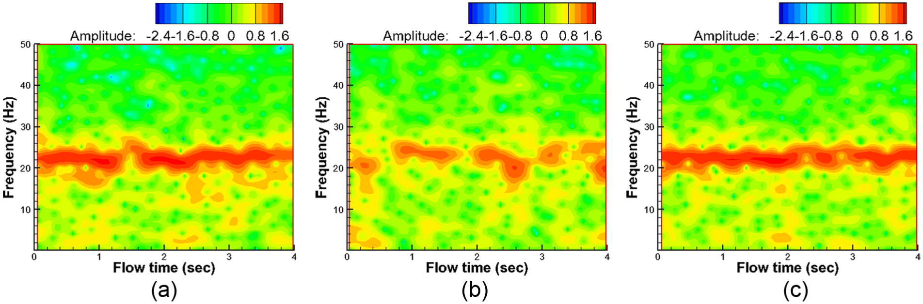
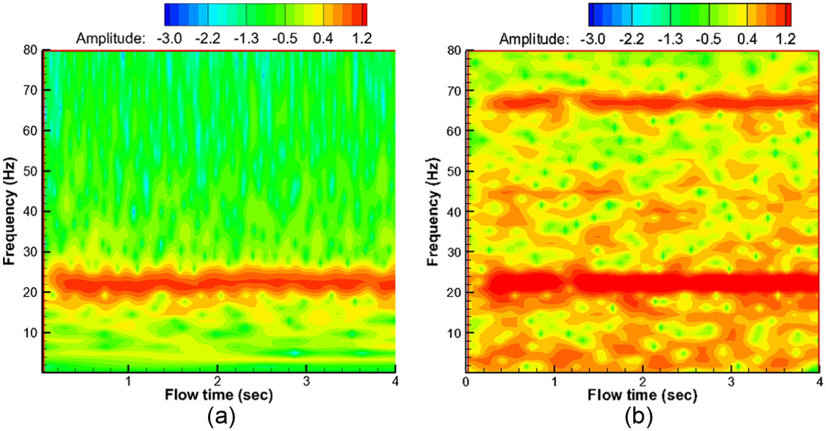
Spectral energy of the local frequency in region 3: (a) Case A, (b) Case B1, and (c) Case B2.

Figure 12 shows the evolution of the predominant frequency, normalized to a experimental value of f* = 22.1 Hz, with respect to the elapsed flow time for Cases B1 and B2, and it explains why the flow structure for Case B2 is expected to resemble that for Case A. The evolution of the normalized frequency for Case B1 changes noticeably and deviates from the reference line, f/f* = 1, especially in region 5, which is near the wall boundary. For Cases A, B1, and B2, Figure 13 further shows how equation (5) is used to obtain the departure from axial flow velocity along the pipe and upstream of the vortex generator. The abscissa in Figure 13 denotes the normalized position away from the forward face of the vortex generator along the pipe centerline. Since both profiles are compared with a fully developed velocity profile, the departure diminishes as represented by a dash line. At far upstream of the vortex generator, ΔV* for Cases B1 and B2 is slightly higher than 0.5. The value of ΔV* decreases slightly as the flow approaches the vortex generator. The flow qualities deteriorate substantially near the front face of the vortex generator. Obviously, the departure from ΔV* for Case B1 is greater than that for Case B2, so Case B2 is more likely to be fully developed. These departures from ΔV* in Figure 13 are related to the evolution of the deviation in the predominant frequency in Figure 12.

Figure 12.

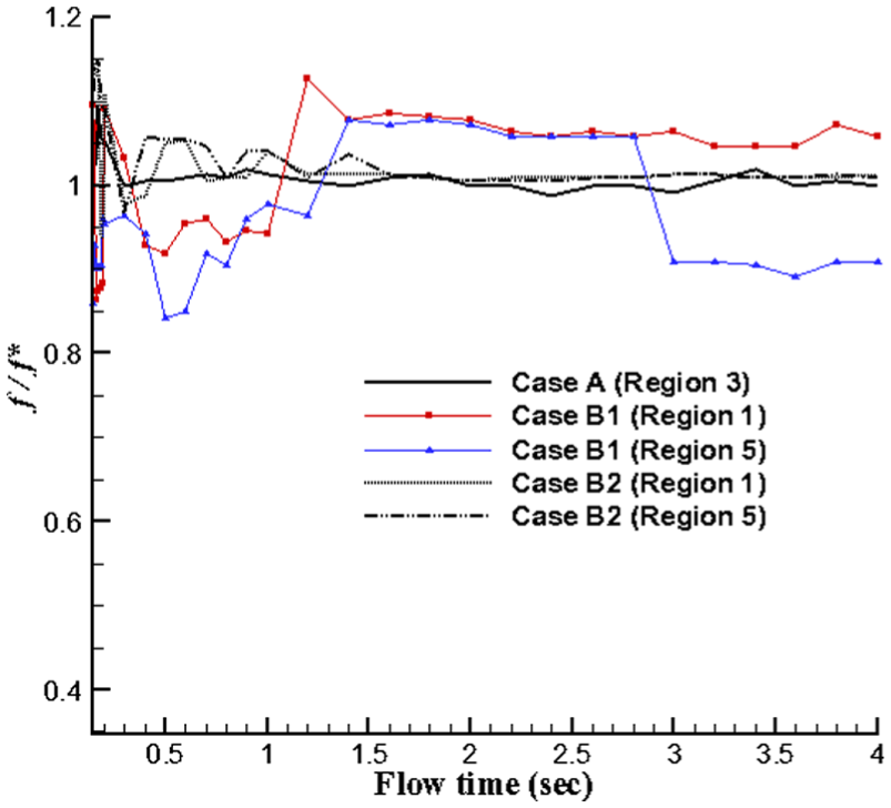
Evolution of the deviation in the predominant frequency for shear flows at inlet.

Figure 13.

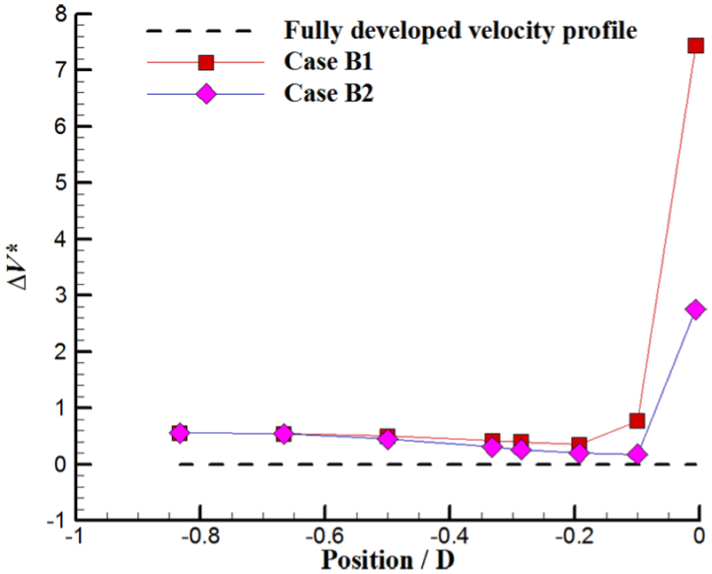
Departure ΔV* along the pipe, from the inlet to the vicinity of the vortex generator.

Unsteady plug flows with sinusoidal profiles

Unsteady inlet flows, in terms of the frequency and amplitude variations, are used to determine the effect of environmental disturbance on vortex shedding for the vortex flowmeter. The benchmark Case C is a plug flow with a uniform flow with a velocity of 3.6 m/s, and it yields the same flow rate as the other cases. Figure 14 shows the frequency spectra for region 1 (left) and region 3 (right). Computational results showed that the predominant frequencies slightly differ from those for Case A in regions 1 and 3. Moreover, Cases C1 and C2 in Figure 15 and Case D in Figure 16, in which the value, ω = 140, is related to the predominant shedding frequency generated in Case C. Cases C1, C2, and D are used to determine the effects of varying amplitude of the sinusoidal inlet flow on the predominant frequency in comparison with Case C. In Case C1, inlet flow amplitude is low, and the predominant frequency slightly changes (from 21.9 to 22.3 Hz) in region 1, but background noise increases in the frequency spectrum. In this case, inlet flow fluctuation is not sustained and does not substantially affect the downstream flow structure or the original predominant frequency. For Case C2, however, in which the inlet flow amplitude increases and the predominant frequency changes from 21.9 to 16.7 Hz in region 1, the frequency spectrum is very different from that for Case C. For Cases C1, C2, and D, Case D with ω = 140 and ε = 0.5 has the largest amplitude and is chosen as the typical case for further comparisons. Figure 16 shows the frequency spectrum for Case D. It is interesting to note that the predominant frequency in region 1 is 11.1 Hz in Case D, and no predominant frequency is found in region 3. In the left side of Figure 16, the third and the fifth harmonics appear at 33.5 and 55.7 Hz, respectively, in addition to the predominant frequency. Table 3 shows the frequency characteristics for Case D along the entire generator. The table shows that all regions except region 3 have distinct predominant and harmonic frequencies (brackets). Obviously, the unsteady inlet flows predominantly affect the vortex shedding frequency if the amplitude is high enough to enhance the flow structure. When the exciting frequency for the inlet flow is 22.29 Hz (ω = 140), the push-forward flow (11.1 Hz) enhances one vortex shedding of the vortex street. Thus, the predominant frequency is 11.1 Hz rather than 22.29 Hz, since each cycle has a pair of shedding vortices. Note that odd-numbered multiples of the first harmonic frequency are present in Figure 16, presumably due to the fact that the present phenomenon is very similar to the acoustic principle for a closed-end column. In Figure 2, the physical model used for the simulation has two boundaries, one of which is the given inlet velocity profile as a closed end, and the other of which is treated as an outflow as an open end. Specifically, a closed-end instrument does not possess even-numbered harmonics. Since only odd-numbered harmonics are produced in Figure 16, the frequency of each harmonic is an odd-numbered multiple of the frequency of the first harmonic.²⁴

Figure 14.

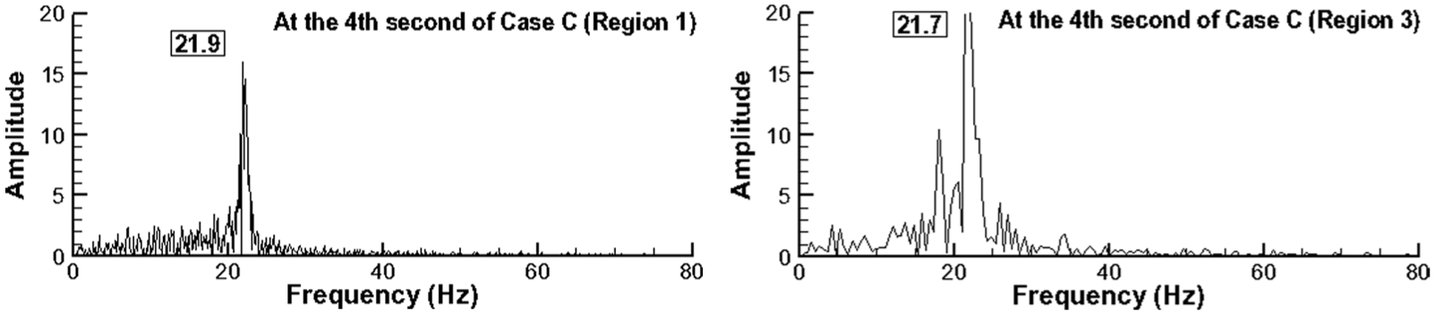
Frequency spectra for Case C in regions 1 (left) and 3 (right).

Figure 15.

Frequency spectra for Cases C1 (first row) and C2 (second row) in regions 1 (left) and 3 (right).

Figure 16.

Frequency spectra for Case D in regions 1 (left) and 3 (right).

Table 3.

Summary of the frequency characteristics for all cases (at the fourth second).

Region	Case
	C1 (ω = 140, ε = 0.1)	C2 (ω = 140, ε = 0.2)	D (ω = 140, ε = 0.5)	D1 (ω = 35, ε = 0.5)	D2 (ω = 70, ε = 0.5)	D3 (ω = 137.5, ε = 0.5)	D4 (ω = 210, ε = 0.5)	D5 (ω = 280, ε = 0.5)
Region 1	22.3	16.7 (5.5)	11.1 (33, 55.7)	26.9 (weak)	11.2 (22.3)	11 (32.8, 54.7)	16.7 (50.2, 83.5)	22.3 (66.9)
Region 2	22.3	16.6 (5.5)	11.2 (33.4, 55.8)	26.9 (weak)	11.2 (22.3)	10.9 (32.8)	16.7 (50.1, 83.5)	22.3 (66.8)
Region 3	22.5	16.6 (5.5)	15.1 (weak)	26.9 (weak)	22.3 (11.2)	12.1 (weak)	16.7 (50.2, 83.5)	22.3 (66.9)
Region 4	22.6	16.7 (5.3)	11.2 (33.5)	26.9 (weak)	22.3 (11.2)	10.9 (32.8)	16.7 (50.2, 83.5)	22.3 (66.9)
Region 5	22.6	16.6 (5.2)	11.2 (33.4, 55.8)	26.9 (weak)	22.3 (11.2)	10.9 (32.8)	16.7 (50.1, 83.5)	22.2 (66.9)

Figure 17 shows the frequency spectra for Cases D1 (the first row), D2 (the second row), D3 (the third row), D4 (the fourth row), and D5 (the fifth row) in region 1 (left column) and region 3 (right column). For ω = 35, that is, the lowest value in all cases, the coherent structure of the vortex shedding is weak, and the predominant frequency is indistinct in region 1 and region 3 (first row in Figure 17). However, when ω = 70, the predominant frequency becomes distinct in region 1 and region 3 and background noise is increased (second row in Figure 17). The predominant frequency, 22.3 Hz, is likely related to that for Case C. Interestingly, the predominant frequency for Case C disappears when ω exceeds 140. Harmonics related to inlet sinusoidal frequency are also observed in Cases D3 (at inlet: ω = 137.5, f = 21.9), D (at inlet: ω = 140, f = 22.3), D4 (at inlet: ω = 210, f = 33.4), and D5 (at inlet: ω = 280, f = 44.6). Notably, the predominant frequency for vortex shedding is half the sinusoidal exciting frequency of the inlet velocity, for each case. That is, f = 11 for Case D3, f = 11.1 for Case D, f = 16.7 for Case D4, and f = 22.3 for Case D5. Again, since the coherent structure of vortex shedding is apparently dominated by inlet flow features, the predominant frequency drops to one half of the value for the inlet as described previously. Figure 18 compares the spectral energy for Cases C and D5 in region 3. Case D5 reveals a distinct predominant frequency and other harmonics resulting from unsteady inflow conditions, which were also observed in the case of a closed-end pipe in acoustics.

Figure 17.

Frequency spectra for Cases D1–D5 (rows 1–5, respectively) in regions 1 (left) and 3 (right).

Figure 18.

Comparison of spectral energy for Cases C (left) and D5 (right) in region 3: (a) Case C and (b) Case D5.

Concluding remarks

Accurately acquiring the predominant frequency of vortex shedding behind the vortex generator is vital for vortex flowmeter applications. This study performed a series of numerical experiments to determine how various inlet flow conditions in a pipe affect the characteristics of the predominant frequency downstream of the vortex generator in the specific vortex flowmeter. Two shear flows are used as steady boundaries at inlet for comparing flow qualities. Simulations show that vortex shedding stabilizes at 4 s. For the shear flow in the spanwise direction at the inlet, the flow quality upstream of the generator is worse because of momentum exchanges from upstream to downstream as well as along the generator. For the shear flow in the transverse direction, the downstream vortex shedding of the vortex generator is more coherent, the evolution of the normalized frequency is more stable, and its velocity profile upstream of the generator is more fully developed.

For unsteady plug flows, the effects on the predominant frequency of vortex shedding are determined in terms of the exciting frequency and amplitude variations at inlet. Comparisons show that background noise in the frequency spectrum increases as amplitude increases, and if the original predominant frequency is changed, harmonics frequencies may appear accordingly. Besides, setting the amplitude at one half of the average velocity results in a distinct predominant frequency as the exciting frequency approaches the original predominant frequency. The predominant frequency is one half of the sinusoidal exciting frequency if the exciting amplitude is high enough to enhance the flow structure. Notably, multiples of the first harmonic frequency are odd-numbered. This phenomenon is very similar to that in a closed-end column in acoustic, in which the frequency of each harmonic is an odd-numbered multiple of the frequency of the first harmonic.

Footnotes

Appendix 1 Acknowledgements

The author wishes to acknowledge Prof. C.Y. Wei, R.O.C. Air Force Academy, for commenting on an early draft and Mr Y.C. Huang, Energy Management System Co., Ltd, for collecting experimental data.

Academic Editor: Chin-Lung Chen

Declaration of conflicting interests

The author(s) declared no potential conflicts of interest with respect to the research, authorship, and/or publication of this article.

Funding

The author(s) disclosed receipt of the following financial support for the research, authorship, and/or publication of this article: Financial assistance for this research is provided by the Taiwanese Ministry of Science and Technology, under contract number NSC100-2622-E-214-005-CC3.

References

Gotthardt

. Mass vortex flowmeter. Meas Control 1995; 172: 182–184.

ISO 5167-1:2003. Measurement of fluid flow by means of pressure differential devices inserted in circular cross-section conduits running full—part 1: general principles and requirements.

Faison

Brickenkamp

. Technical guide for mechanical measurements. US: NIST Handbook 150-2G, Department of Commerce, 2004.

Takamoto

Utsumi

Watanabe

. Installation effects on vortex shedding flowmeters. Flow Meas Instrum 1993; 4: 277–285.

Raisutis

. Investigation of the flow velocity profile in a metering section of an invasive ultrasonic flowmeter. Flow Meas Instrum 2006; 17: 201–206.

ISO/IEC 17025:2005. General requirements for competence of test and calibration laboratories.

. Machine-error testing for various kinds of flowmeters under complicated piping lines (No. EMS-LAB-960816). Tainan, Taiwan: Energy Management System, 2007.

Fletcher

Nicholson

Smith

DJM

. An investigation into the effects of installation on the performance of insertion flowmeters. Flow Meas Instrum 2000; 11: 19–39.

Amadi-Echendu

Zhu

Higham

. Analysis of signals from vortex flowmeters. Flow Meas Instrum 1993; 4: 225–231.

10.

Miau

Yeh

. On measurement uncertainty of a vortex flowmeter. Flow Meas Instrum 2005; 16: 397–404.

11.

Hsiao

Chiang

. Experimental study of cellular shedding vortices behind a tapered circular cylinder. Exp Therm Fluid Sci 1998; 17: 179–186.

12.

Aissa

Bouabdallah

Oualli

. Radial deformation frequency effect on the three-dimensional flow in the cylinder wake. J Fluid Eng 2014; 137: 011104.

13.

Patankar

. Numerical heat transfer and fluid flow. New York: Hemisphere, 1980.

14.

Van Doormaal

Raithby

. Enhancements of the simple method for predicting incompressible fluid flows. Numer Heat Transfer 1984; 7: 147–163.

15.

Achenbach

Heinecke

. On vortex shedding from smooth and rough cylinders in the range of Reynolds numbers 6 × 10³ to 5 × 10⁶. J Fluid Mech 1981; 109: 239–251.

16.

ANSYS. ANSYS FLUENT 13 theory guide. Canonsburg, PA: ANSYS, 2010.

17.

Rodi

. Comparison of LES and RANS calculations of the flow around bluff bodies. J Wind Eng Ind Aerod 1997; 69: 55–75.

18.

Pope

. Turbulent flows. Cambridge: Cambridge University Press, 2003.

19.

Omori

Jakirlić

Tropea

. Shearless and sheared flow past a circular cylinder: comparative analysis by means of LES. Int J Heat Fluid Fl 2008; 29: 703–720.

20.

Miau

. A study on signal quality of a vortex flowmeter downstream of two elbows out-of-plane. Flow Meas Instrum 2002; 13: 75–85.

21.

Schlichting

. Boundary layer theory. New York: McGraw-Hill, 1979.

22.

Jeng

Huang

Cheng

. Decomposition of one-dimensional waveform using iterative Gaussian diffusive filtering methods. P Roy Soc A: Math Phy 2008; 464: 1673–1695.

23.

Parnaudeau

Heitz

Lamballais

. Direct numerical simulations of vortex shedding behind cylinders with spanwise linear nonuniformity. J Turbul 2007; 8: N13.

24.

Benson

. University physics. New York: John Wiley & Sons, 2009.