Output feedback controller design for polynomial linear parameter varying system via parameter-dependent Lyapunov functions

Abstract

This article presents a new output feedback controller design method for polynomial linear parameter varying model with bounded parameter variation rate. Based on parameter-dependent Lyapunov function, the polynomial linear parameter varying system controller design is formulated into an optimization problem constrained by parameterized linear matrix inequalities. To solve this problem, first, this optimization problem is equivalently transformed into a new form with elimination of coupling relationship between parameter-dependent Lyapunov function, controller, and object coefficient matrices. Then, the control solving problem was reduced to a normal convex optimization problem with linear matrix inequalities constraint on a newly constructed convex polyhedron. Moreover, a parameter scheduling output feedback controller was achieved on the operating condition, which satisfies robust performance and dynamic performances. Finally, the feasibility and validity of the controller analysis and synthesis method are verified by the numerical simulation.

Introduction

Most physical systems have significant nonlinear characteristics, which cannot be ignored in many control designs and brought great complexity in system analysis and synthesis.^1–3 In gain-scheduling control for nonlinear objects, classical gain-scheduling controller is constructed from interpolation of local linear controller gains designed by linear time-invariant control theory. This classical gain-scheduling approach does not build theoretical connection among scheduling parameters, control objects, and controller; hence, it cannot theoretically guarantee the stability and performance of control system on the non-designed operating conditions.^4–6 Therefore, the linear parameter varying (LPV) control draws great attention because of the strong ability in nonlinear characteristics’ description for complex objects, guaranteed global stability, and control performance. ⁷

Based on Lyapunov theory, the analysis and synthesis methods for LPV control are typically focused on the construction of Lyapunov functions. Motivated by building the theoretical connection between the scheduling parameter and the controller, the parameter-dependent Lyapunov function (PLF) is introduced into the LPV control framework with reduced conservativeness compared with parameter-independent Lyapunov function. Wu et al. ⁸ used PLF for state-space parameter-dependent plant control with satisfying L₂ norm performance. G Chesi et al. ⁹ formulated a sufficient condition for the existence of a homogeneous polynomial Lyapunov function into a linear matrix inequality (LMI) feasibility problem for a system with time-varying structured uncertainties. G Chesi et al. ¹⁰ also analyzed robust stability of time-varying polytopic systems by parameter-dependent homogeneous Lyapunov functions. D Henrion et al. ¹¹ analyzed a linear system robust stability affected by real parametric uncertainty via quadratic polynomial Lyapunov functions. M Sato^12,13 and Sato and Peaucelle ¹⁴ designed filter for LPV systems using quadratic PLFs and gain-scheduled output feedback controllers via PLFs. M Ait Rami et al. ¹⁵ studied the stabilization for LPV-positive systems with PLF combined with a slack variable on the simplex set. G Cai et al. ¹⁶ designed a gain-scheduled H₂ controller for continuous-time polytopic LPV systems employing a basis PLF and some slack variables to performance conditions. S Chumalee and Whidborne ¹⁷ designed a gain-scheduled output feedback H_∞ controller via PLFs for affine LPV models.

Recent studies combining the conception of PLF with polynomial form and LMI technique lead to considerable progress in flexibility and accuracy of LPV system controller design. But the design of this controller is a nonconvex optimization problem which is difficult to be solved. Then, the analysis and synthesis methods are typically focused on converting the optimization problem into convex optimization problem with parameter-dependent LMI constraints and the calculating methods. ¹⁸ F Wu et al. ⁸ designed induced L₂ controller for LPV systems with bounded parameter variation rates by gridding method. JA Turso and JS Litt ¹⁹ used the same gridding method to design the robust controller for deteriorated turbofan engines. PA Bliman ²⁰ studied the existing conditions for polynomial solutions of parameter-dependent LMIs, which can be used in parametric robustness or gain-scheduling issues. PJ De Oliveira et al. ²¹ presented an LMI approach to compute H_∞ guaranteed costs by means of PLFs on polytope-type domains. RCLF Oliveira et al.^22,23 provided a homogeneous polynomial solution by relaxation method for parameter-dependent LMIs defined on the unit simplex and multi-simplex. RCLF Oliveira et al. ²⁴ also studied the LMI relaxations for robust H₂ performance analysis on polytopic linear systems. CM Agulhari et al. ²⁵ designed a reduced-order robust controller for uncertain linear systems by a two-staged LMI relaxation method. G Chesi ²⁶ provided an exact LMI condition for robust asymptotic stability of uncertain systems depending polynomially on a scalar parameter in both continuous-time and discrete-time cases. P Gahinet et al. ²⁷ and T Azuma et al. ²⁸ developed a multiconvexity method to deal with this problem by constructing convex polyhedron and to design the controller on the vertex. However, the analysis result achieved by gridding method does not have the global characteristics; the relaxation method can guarantee the global characters of analysis result, but the significance of relaxation index is not clear, which leads to the difficulty in control system synthesis; the multiconvexity method is for general LPV model with hyper-rectangle parameter space; when applying on models such as polynomial linear parameter varying (PLPV) model with polynomial curve parameter space, it will increase conservativeness in control system synthesis.

In this note, for the PLPV model with bounded parameter variation rate, the parameterized linear matrix inequality (PLMI) conditions guaranteeing robust performance are studied for PLF-based controller design. Then, to overcome the aforesaid problems in controller solving process, this optimization design conditions are transformed into a new form with decoupled relationship between PLF and controller. Then, the global controller solving problem is reduced to a normal convex optimization problem on certain convex polyhedron. ²⁸ Moreover, the derivative information of polynomial curve parameter space is used to build an improved convex polyhedron construction method, which effectively reduces the conservativeness in controller solution. Finally, a numerical simulation on PLPV model validates the controller design method.

Problem formulation

An output feedback control system design problem is described for an expanded PLPV model. Then, the PLF conception is introduced for the sake of control system analysis and synthesis.

PLPV model and introduction of PLF

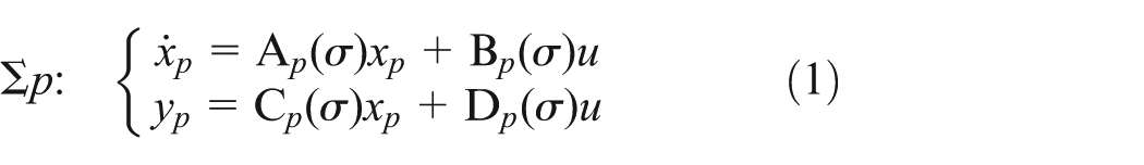
Consider the following PLPV model $\mathrm{\Sigma }p$ , which depends on the parameter $\sigma$ with bounded parameter variation rate ²⁷

$$\mathrm{\Sigma }p:\{\begin{array}{c}{\stackrel{.}{x}}_p={\mathrm{A}}_p(\sigma )x_p+{\mathrm{B}}_p(\sigma )u\\ y_p={\mathrm{C}}_p(\sigma )x_p+{\mathrm{D}}_p(\sigma )u\end{array}$$

(1)

where $x_p\in {\mathrm{R}}^{{\mathrm{n}}_1}$ is the state vector, $u\in {\mathrm{R}}^{{\mathrm{n}}_2}$ is the input vector, and $y_p\in {\mathrm{R}}^{{\mathrm{n}}_3}$ is the output vector. The coefficient matrices of system (1) have the same form, which is defined as follows

$$\ell (\sigma )={\displaystyle \sum _{i=0}^{\mathrm{g}}{\sigma }^i{\ell }_i},\sigma \in [{\sigma }_{\min },{\sigma }_{\max }],\left|\stackrel{.}{\sigma }\right|<D_{\max }$$

(2)

where ${\ell }_i$ are the known real constant matrices with appropriate dimensions. Moreover, we consider the following form of PLF needed in system analysis and synthesis

$$\mathrm{V}(x,\sigma )=x^{\mathrm{T}}\mathrm{P}(\sigma )x,\mathrm{P}(\sigma )={\displaystyle \sum _{i=0}^{\mathrm{m}}{\sigma }^i{\mathrm{P}}_i}$$

(3)

where $\mathrm{P}(\sigma )$ is a symmetric positive definite polynomial Lyapunov matrix of degree m, and P _i is a symmetric real constant matrix with appropriate dimensions.

Control system for PLPV model

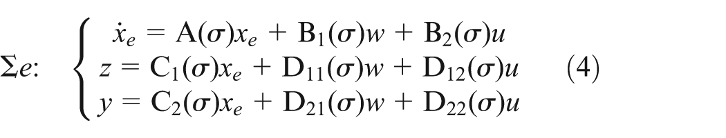
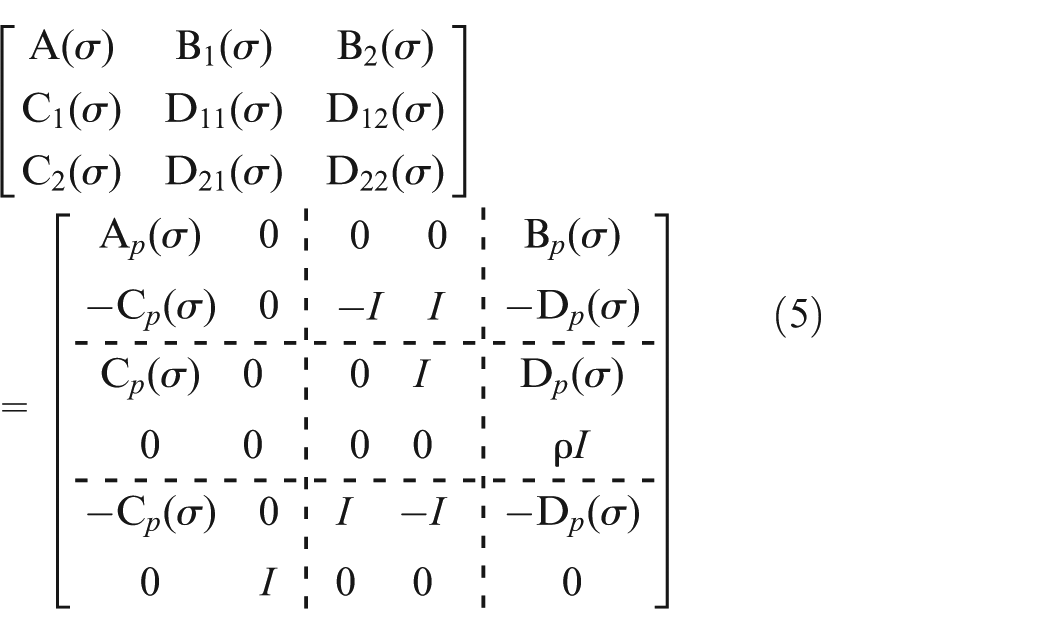
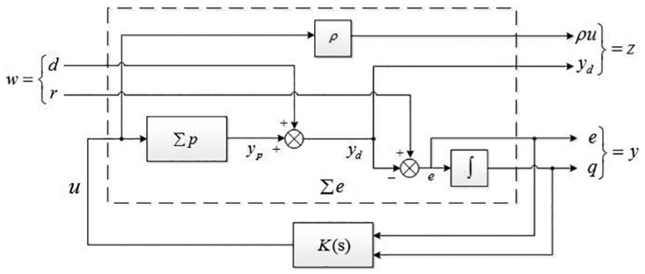
The interconnection diagram of LPV control system is proposed in Figure 1. Where K(s) is the controller which depends on parameter $\sigma$ ; $\mathrm{\Sigma }e$ shown in dashed border is the expanded control object; $w=(d,r)\in {\mathrm{R}}^{2{\mathrm{n}}_3}$ is the input of expanded control system, where d is the external disturbance and r is the control expectation; $z=(y_d,\rho u)\in {\mathrm{R}}^{({\mathrm{n}}_2+{\mathrm{n}}_3)}$ is the output, where $y_d=y_p+d$ , $\rho$ is the weight of u, and $y=(e,q)\in {\mathrm{R}}^{2{\mathrm{n}}_3}$ . Consider $\stackrel{·}{q}=e=r-y_d$ and $q={\int }_0^{\mathrm{t}}r(\tau )-{\mathbf{y}}_d(\tau )\mathrm{d}\tau$ , define $x_e=(x_p,q{)}^{\mathrm{T}}\in {\mathrm{R}}^{({\mathrm{n}}_1+{\mathrm{n}}_3)}$ as the expanded state vector. Then, we get ²⁹

$$\mathrm{\Sigma }e:\{\begin{array}{c}{\stackrel{·}{x}}_e=\mathrm{A}(\sigma )x_e+{\mathrm{B}}_1(\sigma )w+{\mathrm{B}}_2(\sigma )u\hfill \\ \multicolumn{1}{c}{z={\mathrm{C}}_1(\sigma )x_e+{\mathrm{D}}_{11}(\sigma )w+{\mathrm{D}}_{12}(\sigma )u}\\ \multicolumn{1}{c}{y={\mathrm{C}}_2(\sigma )x_e+{\mathrm{D}}_{21}(\sigma )w+{\mathrm{D}}_{22}(\sigma )u}\end{array}$$

(4)

where

$$\left[\begin{array}{ccc}A(\sigma )& B_1(\sigma )& B_2(\sigma )\\ C_1(\sigma )& D_{11}(\sigma )& D_{12}(\sigma )\\ C_2(\sigma )& D_{21}(\sigma )& D_{22}(\sigma )\end{array}\right]=\left[\begin{array}{ccc}\begin{array}{cc}{A}_p(\sigma )& 0\\ -C_p(\sigma )& 0\end{array}& \begin{array}{cc}0& 0\\ -I& I\end{array}& \begin{array}{c}{B}_p(\sigma )\\ -D_p(\sigma )\end{array}\\ \begin{array}{cc}{C}_p(\sigma )& 0\\ 0& 0\end{array}& \begin{array}{cc}0& I\\ 0& 0\end{array}& \begin{array}{c}{D}_p(\sigma )\\ \rho I\end{array}\\ \begin{array}{cc}-C_p(\sigma )& 0\\ 0& I\end{array}& \begin{array}{cc}I& -I\\ 0& 0\end{array}& \begin{array}{c}-D_p(\sigma )\\ 0\end{array}\end{array}\right]$$

(5)

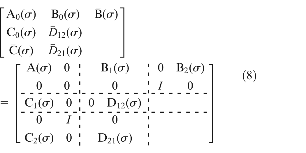
where I stands for unit matrix with appropriate dimensions.

Figure 1.

Block diagram of LPV control system.

According to equation (4), the transfer function matrix from control expectation w to output z can be obtained using the control law as $u=K(s)y$ , and $K(\sigma )$ can be defined as follows

$$K(s):\{\begin{array}{c}{\stackrel{·}{x}}_{\mathrm{K}}={\mathrm{A}}_{\mathrm{K}}(\sigma )x_{\mathrm{K}}+{\mathrm{B}}_{\mathrm{K}}(\sigma )y\hfill \\ \multicolumn{1}{c}{u={\mathrm{C}}_{\mathrm{K}}(\sigma )x_{\mathrm{K}}+{\mathrm{D}}_{\mathrm{K}}(\sigma )y}\end{array},K(\sigma )=\left[\begin{array}{cc}{\mathrm{A}}_{\mathrm{K}}(\sigma )\hfill & {\mathrm{B}}_{\mathrm{K}}(\sigma )\hfill \\ \multicolumn{1}{c}{{\mathrm{C}}_{\mathrm{K}}(\sigma )}& {\mathrm{D}}_{\mathrm{K}}(\sigma )\hfill \end{array}\right]$$

(6)

where $x_{\mathrm{K}}\in {\mathrm{R}}^{{\mathrm{n}}_4}$ is the state vector of controller, and the coefficient matrices rely on parameter $\sigma$ with bounded parameter variation rate in form (2). Let $x_c=(x_e,x_{\mathrm{K}})$ be the state vector of closed-loop system, and considering the expanded system (4) with controller (6), the closed-loop system is described as follows

$$\mathrm{\Sigma }c:\{\begin{array}{c}{\stackrel{·}{x}}_c={\mathrm{A}}_{\mathrm{c}}(\sigma )x_{\mathbf{c}}+{\mathrm{B}}_{\mathrm{c}}(\sigma )w\hfill \\ \multicolumn{1}{c}{z={\mathrm{C}}_{\mathrm{c}}(\sigma )x_{\mathbf{c}}+{\mathrm{D}}_{\mathrm{c}}(\sigma )w}\end{array}$$

(7)

If we define the following coefficient matrices

$$\left[\begin{array}{ccc}{A}_0(\sigma )& B_0(\sigma )& \overline{B}(\sigma )\\ C_0(\sigma )& {\overline{D}}_{12}(\sigma )& \\ \overline{C}(\sigma )& {\overline{D}}_{21}(\sigma )& \end{array}\right]=\left[\begin{array}{ccc}\begin{array}{cc}A(\sigma )& 0\\ 0& 0\end{array}& \begin{array}{c}{B}_1(\sigma )\\ 0\end{array}& \begin{array}{cc}0& B_2(\sigma )\\ I& 0\end{array}\\ \begin{array}{cc}{C}_1(\sigma )& 0\end{array}& \begin{array}{cc}0& D_{12}(\sigma )\end{array}& \begin{array}{cc}& \end{array}\\ \begin{array}{cc}0& I\\ C_2(\sigma )& 0\end{array}& \begin{array}{c}0\\ D_{21}(\sigma )\end{array}& \begin{array}{cc}& \\ & \end{array}\end{array}\right]$$

(8)

Then, the coefficient matrices of closed-loop system can be expressed as affine functions about $K(\sigma )$ given in equation (9)

$$\left[\begin{array}{cc}{A}_c(\sigma )& B_c(\sigma )\\ C_c(\sigma )& D_c(\sigma )\end{array}\right]=\left[\begin{array}{cc}{A}_0(\sigma )+\overline{B}(\sigma )K(\sigma )\overline{C}(\sigma )& B_0(\sigma )+\overline{B}(\sigma )K(\sigma ){\overline{D}}_{21}(\sigma )\\ C_0(\sigma )+{\overline{D}}_{12}(\sigma )K(\sigma )\overline{C}(\sigma )& D_{11}(\sigma )+{\overline{D}}_{12}(\sigma )K(\sigma ){\overline{D}}_{21}(\sigma )\end{array}\right]$$

(9)

Control system analysis and design of PLPV system

Define $J=\Vert G_{\mathrm{zw}}{\Vert }_{\infty }$ as H_∞ performance target function of system (7). Then, the PLPV system controller design problem we addressed here is as follows: for PLPV model (1), we design the controller K(s) that assures the stability of control system (7) and minimizes the performance target function J. According to the Lyapunov stability theory, PLF, and the bounded real lemma, the following theorem is given.^8,20

Theorem 1

For a given positive real number $\gamma >0$ , system (7) is stable, its H_∞ performance target function $J<\gamma$ , if there exist positive definite matrices $\mathrm{P}(\sigma )={\mathrm{P}}^T(\sigma )$ and $K(\sigma )$ that can satisfy equation (10) on all admissible trajectories of parameter $\sigma$ with bounded varying rate $\begin{array}{c}\left|\stackrel{·}{\sigma }\right|<D_{max}\hfill \end{array}$

$$\begin{array}{c}[\begin{array}{c}{({\mathrm{A}}_0(\sigma )+\overline{\mathrm{B}}(\sigma )K(\sigma )\overline{C}(\sigma ))}^T\mathrm{P}(\sigma )+\mathrm{P}(\sigma )({\mathrm{A}}_0(\sigma )+\overline{\mathrm{B}}(\sigma )K(\sigma )\overline{C}(\sigma ))+\stackrel{·}{\mathrm{P}}(\sigma )\hfill \\ \multicolumn{1}{c}{*}\\ \multicolumn{1}{c}{*}\end{array}\hfill \\ \begin{array}{cc}\mathrm{P}(\sigma )({\mathrm{B}}_0(\sigma )+\overline{\mathrm{B}}(\sigma )K(\sigma ){\overline{\mathrm{D}}}_{21}(\sigma ))\hfill & {({\mathrm{C}}_0(\sigma )+{\overline{\mathrm{D}}}_{12}(\sigma )K(\sigma )\overline{\mathrm{C}}(\sigma ))}^T\hfill \\ \multicolumn{1}{c}{-\gamma I}& {({\mathrm{D}}_{11}(\sigma )+{\overline{\mathrm{D}}}_{12}(\sigma )K(\sigma ){\overline{\mathrm{D}}}_{21}(\sigma ))}^T\hfill \\ \multicolumn{1}{c}{*}& -\gamma I\hfill \end{array}]<0\hfill \end{array}$$

(10)

where $\mathrm{P}(\sigma )=\sum ^{\mathrm{m}}{\sigma }^i{\mathrm{P}}_i$ , $\stackrel{·}{\mathrm{P}}(\sigma )=\sum ^{\mathrm{m}}i{\sigma }^{i-1}{D}_{max}{\mathrm{P}}_i$ .

Theorem 1 converts the PLPV formed controller design problem into a PLMI constrained optimization problem on a minimal value of $\gamma$ , but this kind of constraint includes infinite number of PLMI constraints and contains the coupling product of $\mathrm{P}(\sigma )$ , $K(\sigma )$ , and system coefficient matrices. Then, this optimization problem cannot be solved with normal LMI constrained convex optimization technique accurately. What is more, the key of the controller design is to solve the global controller optimization problem with minimal conservativeness. Then, a two-staged method is studied to resolve this problem: first, eliminate the coupling relationship between $\mathrm{P}(\sigma )$ and $K(\sigma )$ ; second, considering the geometry characters of parameter curve of PLMI condition (10), a new solving method for PLMI constrained optimization problem is given using a convex polyhedron construction approach. Then, by means of the following theorem, the PLMI constraints can be reformulated in a new form without coupling between $\mathrm{P}(\sigma )$ and $K(\sigma )$ .

Theorem 2

For a given positive real number $\gamma >0$ , system (7) is stable, its H_∞ performance target function $J<\gamma$ , if there exist positive definite matrices $X(\sigma )=X^{\mathrm{T}}(\sigma )$ and $Y(\sigma )=Y^{\mathrm{T}}(\sigma )$ that can satisfy equation (11) on all admissible trajectories of parameter $\sigma$ with bounded varying rate $\begin{array}{c}\left|\stackrel{·}{\sigma }\right|<D_{max}\hfill \end{array}$

$$\left[\begin{array}{cc}X(\sigma )\hfill & I\hfill \\ \multicolumn{1}{c}{*}& Y(\sigma )\hfill \end{array}\right]\ge 0$$

(11a)

$${\left[\begin{array}{cc}{N}_x(\sigma )& 0\\ *& I\end{array}\right]}^T\left[\begin{array}{ccc}{A}^T(\sigma )X(\sigma )+X(\sigma )A(\sigma )+\stackrel{.}{X}(\sigma )& X(\sigma )B_1(\sigma )& C_1{(\sigma )}^T\\ *& -I& D_{11}{(\sigma )}^T\\ *& *& -I\end{array}\right]\left[\begin{array}{cc}{N}_x(\sigma )& 0\\ *& I\end{array}\right]<0$$

(11b)

$${\left[\begin{array}{cc}{N}_y(\sigma )& 0\\ *& I\end{array}\right]}^T\left[\begin{array}{ccc}A(\sigma )Y(\sigma )+Y(\sigma )A{(\sigma )}^T+\stackrel{.}{Y}(\sigma )& Y(\sigma )C_1^T(\sigma )& B_1(\sigma )\\ *& -I& D_{11}(\sigma )\\ *& *& -I\end{array}\right]\left[\begin{array}{cc}{N}_y(\sigma )& 0\\ *& I\end{array}\right]<0$$

(11c)

where $X(\sigma )=\sum _{i=0}^{\mathrm{m}}{\sigma }^i{X}_i$ , $\stackrel{·}{X}(\sigma )=\sum _{i=1}^{\mathrm{m}-1}i{\sigma }^{i-1}{D}_{max}{X}_i$ , $Y(\sigma )=\sum _{i=0}^{\mathrm{m}}{\sigma }^i{Y}_i$ , and $\stackrel{·}{Y}(\sigma )=\sum _{i=1}^{\mathrm{m}-1}i{\sigma }^{i-1}{D}_{max}{Y}_i$ . Denote $N_x(\sigma )$ and $N_y(\sigma )$ as the basis of kernel space $\ker ([\begin{array}{cc}{C}_2(\sigma )\hfill & D_{21}(\sigma )\hfill \end{array}])$ and $\ker ([\begin{array}{cc}{B}_2^{\mathrm{T}}(\sigma )\hfill & D_{12}^{\mathrm{T}}(\sigma )\hfill \end{array}])$ , respectively, which depend on the parameter $\sigma$ .

Then, defining M satisfied $X-Y^{-1}=M{M}^{\mathrm{T}}$ which can be solved by singular value decomposition, a matrix P is constructed

$$\mathrm{P}=\left[\begin{array}{cc}X\hfill & M^{\mathrm{T}}\hfill \\ \multicolumn{1}{c}{*}& I\hfill \end{array}\right]$$

(12)

Considering the constant matrix P and Theorem 1, the PLMI constrained optimization problem (10) has only one variable $K(\sigma )$ , which can be achieved by solving the optimization problem about $\sigma$ given online.

Although Theorem 2 eliminates the coupling relationship between $\mathrm{P}(\sigma )$ and $K(\sigma )$ , the LMI-formed condition (11) is not easy to be resolved because of the PLMI constraints. In this article, an approach solving this optimization problem is given based on a new convex polyhedron construction method. The following theorems are proposed as the basis of solving method.

Convex polyhedron construction–based controller design

For PLPV model, the PLF reduces the control system analysis and synthesis problem into an optimization problem with the PLMI constraints. To guarantee the global characters of controller design, we convert it into a normal convex optimization problem with LMI constraints based on a methodology of convex polyhedron construction; then, the derivative information of PLMI parameter curve is used to formulate a convex polyhedron construction, which can improve the computing efficiency and reduce the conservative of the controller design. ²⁸

Controller solving method based on convex polyhedron construction

Suppose ${\Phi }_{\mathrm{X}}=(X_0,\dots ,X_{\mathrm{m}}{)}^{\mathrm{T}}$ and ${\Phi }_{\mathrm{Y}}=(Y_0,\dots ,Y_{\mathrm{m}}{)}^{\mathrm{T}}$ , considering equations (2) and (3), if $N_x(\sigma )$ and $N_y(\sigma )$ are assumed to be constant matrix, then constraints (11) can be written as

$$\mathrm{F}(\sigma )=\sum _{i=0}^{\mathrm{m}}{\sigma }^i{\mathrm{F}}_i({\Phi }_{\mathrm{X}},{\Phi }_{\mathrm{Y}},\gamma )<0$$

(13)

where ${\mathrm{F}}_i({\Phi }_{\mathrm{X}},{\Phi }_{\mathrm{Y}},\gamma )$ is a symmetric matrix function that affinely depends on ${\Phi }_{\mathrm{X}}$ , ${\Phi }_{\mathrm{Y}}$ , and $\gamma$ . For equation (13), we have the following theorem.

Theorem 3

In m-dimensional linear space, suppose ${\Phi }_{\mathrm{P}}=({\mathrm{P}}_0,\dots ,{\mathrm{P}}_{\mathrm{m}}{)}^{\mathrm{T}}$ satisfying equation (3), assume that there exists a convex polyhedron H₀ including curve $\mathrm{\Gamma }$ defined as ²⁸

$$\mathrm{\Gamma }=\{(\sigma ,\dots ,{\sigma }^{\mathrm{m}}{)}^{\mathrm{T}}|\sigma \in [{\sigma }_{\min },{\sigma }_{\max }]\}$$

(14)

$p^j\in {\mathrm{R}}^{\mathrm{m}}$ and the vertex set of H₀ is ${\mathrm{V}}_0=\{p^j|j=1,\dots ,\mathrm{q}\}$ . If there exist ${\Phi }_{\mathrm{P}}$ and $\gamma$ that satisfy equation (15)

$$\overline{F}(p^j)=\sum _{i=0}^{\mathrm{m}}{p}^j(i)F_i({\Phi }_{\mathrm{P}},\gamma )<0,\forall p^j\in {\mathrm{V}}_0$$

(15)

where $p^j(i)$ is the jth dimension coordinate of $p^j$ , then equation (13) will be satisfied on $\mathrm{\Gamma }$ .

Based on Theorems 2 and 3, the global controller design can be achieved by satisfying equation (15) on the constructed convex polyhedron vertex set. Theorem 3 also indicates the following two facts: the construct convex polyhedron is not unique; in Theorem 3, in order to make equation (13) true on $\mathrm{\Gamma }$ , equation (13) is forced to hold true on H₀ which means the parameter space is expended with the increase in conservativeness. Moreover, how tightly the constructed convex polyhedron includes the parameter curve $\mathrm{\Gamma }$ can affect the conservativeness and accuracy of system analysis and synthesis directly. ²⁸ Then, the following convex polyhedron construction method is given.

Convex polyhedron construction and reformulation of controller design optimization problem

To reduce the conservative caused by convex polyhedron construction, derivative information of the parameter curve is used to build new convex polyhedrons that include the parameter curve piecewise. So unnecessary expansion of parameter space can be reduced to as minimum as possible with the increased number of parameter curve division.

In S-dimensional linear space, the convex polyhedron construction algorithm will be shown on parameter curve $\mathrm{\Gamma }$ .

• Step 1. Suppose ${\alpha }_i={\sigma }_{\min }+(i-1)({\sigma }_{\max }-{\sigma }_{\min })/\mathrm{d}$ and ${\beta }_i={\sigma }_{\min }+i({\sigma }_{\max }-{\sigma }_{\min })/\mathrm{d}$ . Divide the domain of parameter $\sigma$ into d equal parts. Then, the division $\{{\mathrm{\Theta }}_1,\dots ,{\mathrm{\Theta }}_{\mathrm{d}}\}$ is defined as

  $${\mathrm{\Theta }}_i=\{\sigma |\sigma \in [{\alpha }_i,{\beta }_i]\},(i=1,\dots ,\mathrm{d})$$

  (16)

• Step 2. Define the segments ${\mathrm{\Gamma }}_i$ on ${\mathrm{\Theta }}_i$

  $${\mathrm{\Gamma }}_i=\{(\sigma ,\dots ,{\sigma }^{\mathrm{S}}{)}^{\mathrm{T}}|\sigma \in {\mathrm{\Theta }}_i\},(i=1,\dots ,\mathrm{d})$$

  (17)

• Step 3. For each ${\mathrm{\Gamma }}_i$ , the corresponding convex polyhedron ${\mathrm{H}}_i(i=1,\dots ,\mathrm{d})$ is constructed. Then, the vertex set of H _i is $\{p_i^j|j=1,\dots ,\mathrm{s}+1\}$

  $$\{\begin{array}{c}{P_i}^1=({\alpha }_i,{\alpha }_i^2,\dots ,{{\alpha }_i}^{\mathrm{s}}{)}^{\mathrm{T}}\hfill \\ \multicolumn{1}{c}{{P_i}^{\mathrm{s}+1}=({\beta }_i,{\beta }_i^2,\dots ,{{\beta }_i}^{\mathrm{s}}{)}^{\mathrm{T}}}\\ \multicolumn{1}{c}{{\mathrm{P}}_i^j=P_i^{j-1}+(P_i^{\mathrm{s}+1}(j-1)-{\mathrm{P}}_i^1(j-1)-K(j-1){\beta }_i^{j-2})e_{j-1}}\\ \multicolumn{1}{c}{(j=2,\dots ,\mathrm{s})}\\ \multicolumn{1}{c}{k=[P_i^{s+1}(\mathrm{s})-P_i^1(\mathrm{s})](\mathrm{s}{\beta }_i^{s-1}{)}^{-1}}\end{array}$$

  (18)

  where $e_{j-1}$ is the unit coordinate vector and the $(j-1)\mathrm{th}$ dimension coordinate is 1.

• Step 4. Let convex polyhedron $\Psi =\{{\mathrm{H}}_i|i=1,\dots ,\mathrm{d}\}$ , and its vertex set is given by

  $${\mathrm{V}}_1=\{p_i^j|i=1,\dots ,\mathrm{d};j=1,\dots ,\mathrm{s}+1\}$$

  (19)

H is the convex hull of $\Psi$ , and its vertex set is $\mathrm{V}=\{{\nu }_i|i=1,\dots ,N\}$ satisfying $\mathrm{V}\in {\mathrm{V}}_1$

$$\mathrm{H}=\mathrm{Co}({\mathrm{H}}_1\cup {\mathrm{H}}_2\cup ,\dots ,{\mathrm{H}}_{\mathrm{d}})$$

(20)

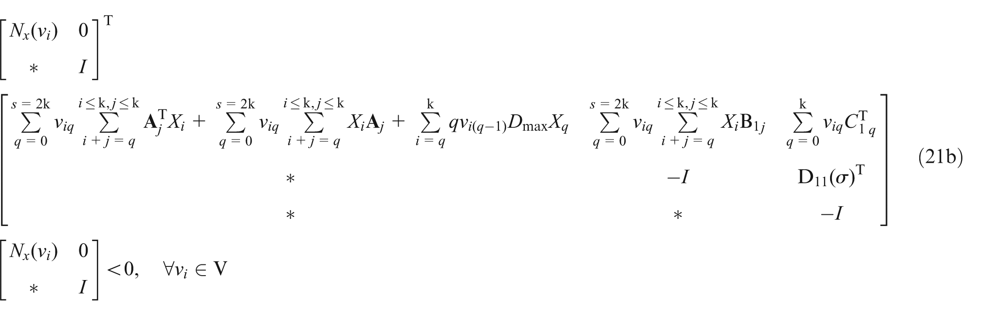
The vertex number N depends on the division number d. It is obvious that H is a convex polyhedron which includes parameter curve $\mathrm{\Gamma }$ . But the proof is not mentioned here as per the scope of this article. In Theorem 2, $N_x(\sigma )$ and $N_y(\sigma )$ describe the parts of the control system that cannot be observed and controlled, respectively. Then, an approximate and simple method is to treat them as constant in equation (11), and a specific value can be calculated on vertex set. Then, according to Theorem 3, condition (11) can be reformulated as equation (21)

$$\left[\begin{array}{cc}\sum _{q=0}^{\mathrm{k}}{v}_{\mathrm{iq}}{X}_q\hfill & I\hfill \\ \multicolumn{1}{c}{*}& \sum _{q=0}^{\mathrm{k}}{v}_{\mathrm{iq}}{Y}_q\hfill \end{array}\right]\ge 0,\forall v_i\in \mathrm{V}$$

(21a)

$$\begin{array}{c}{\left[\begin{array}{cc}{N}_x(v_i)\hfill & 0\hfill \\ \multicolumn{1}{c}{*}& I\hfill \end{array}\right]}^{\mathrm{T}}\hfill \\ \left[\begin{array}{ccc}\sum _{q=0}^{s=2\mathrm{k}}{v}_{\mathrm{iq}}\sum _{i+j=q}^{i\le \mathrm{k},j\le \mathrm{k}}{\mathbf{A}}_j^{\mathrm{T}}{X}_i+\sum _{q=0}^{s=2\mathrm{k}}{v}_{\mathrm{iq}}\sum _{i+j=q}^{i\le \mathrm{k},j\le \mathrm{k}}{X}_i{\mathbf{A}}_j+\sum _{i=q}^{\mathrm{k}}q{v}_{i(q-1)}{D}_{max}{X}_q\hfill & \sum _{q=0}^{s=2\mathrm{k}}{v}_{\mathrm{iq}}\sum _{i+j=q}^{i\le \mathrm{k},j\le \mathrm{k}}{X}_i{{\mathrm{B}}_1}_j\hfill & \sum _{q=0}^{\mathrm{k}}{v}_{\mathrm{iq}}{C_1^{\mathrm{T}}}_q\hfill \\ \multicolumn{1}{c}{*}& -I\hfill & {\mathrm{D}}_{11}{(\sigma )}^{\mathrm{T}}\hfill \\ \multicolumn{1}{c}{*}& *\hfill & -I\hfill \end{array}\right]\hfill \\ \left[\begin{array}{cc}{N}_x(v_i)\hfill & 0\hfill \\ \multicolumn{1}{c}{*}& I\hfill \end{array}\right]<0,\forall v_i\in \mathrm{V}\hfill \end{array}$$

(21b)

$$\begin{array}{c}{\left[\begin{array}{cc}{N}_Y(v_i)\hfill & 0\hfill \\ \multicolumn{1}{c}{*}& I\hfill \end{array}\right]}^{\mathrm{T}}\hfill \\ \left[\begin{array}{ccc}\sum _{q=0}^{s=2\mathrm{k}}{v}_{\mathrm{iq}}\sum _{i+j=q}^{i\le \mathrm{k},j\le \mathrm{k}}{\mathbf{A}}_j^{\mathrm{T}}{Y}_i+\sum _{q=0}^{s=2\mathrm{k}}{v}_{\mathrm{iq}}\sum _{i+j=q}^{i\le \mathrm{k},j\le \mathrm{k}}{Y}_i{\mathbf{A}}_j+\sum _{i=q}^{\mathrm{k}}q{v}_{i(q-1)}{D}_{max}{Y}_q\hfill & \sum _{q=0}^{s=2\mathrm{k}}{v}_{\mathrm{iq}}\sum _{i+j=q}^{i\le \mathrm{k},j\le \mathrm{k}}{Y}_i{{\mathrm{C}}_1}_j^{\mathrm{T}}\hfill & \sum _{q=0}^{\mathrm{k}}{v}_{\mathrm{iq}}{{\mathrm{B}}_1}_q\hfill \\ \multicolumn{1}{c}{*}& -I\hfill & {\mathrm{D}}_{11}{(\sigma )}^{\mathrm{T}}\hfill \\ \multicolumn{1}{c}{*}& *\hfill & -I\hfill \end{array}\right]\hfill \\ \left[\begin{array}{cc}{N}_Y(v_i)\hfill & 0\hfill \\ \multicolumn{1}{c}{*}& I\hfill \end{array}\right]<0,\forall v_i\in \mathrm{V}\hfill \end{array}$$

(21c)

where $v_{i0}=1$ and $v_{\mathrm{iq}}$ , $q\in (1,\dots ,\mathrm{s})$ , is the qth dimensional coordinate of the constructed convex polyhedron vertex $v_i$ . Then, the controller design problem for PLPV model in Theorem 1 with constraints (11) can be reduced to a normal LMI constrained convex optimization problem as follows

$$\{\begin{array}{c}\min \gamma \hfill \\ \multicolumn{1}{c}{\mathrm{s}.\mathrm{t}.\overline{\mathrm{F}}({\nu }_i)=\sum _{q=0}^{\mathrm{s}}{\nu }_{\mathrm{iq}}{F}_q({\Phi }_{\mathrm{X}},{\Phi }_{\mathrm{Y}},\gamma )<0,\forall {\nu }_i\in \mathrm{V}}\end{array}$$

(22)

Controller design method for PLPV system

According to the aforesaid theory, following are the steps of output feedback controller design method for PLPV model using PLF:

• Step 1. Build the expanded control system (5) based on PLPV model (1).

• Step 2. Construct the convex polyhedron H.

• Step 3. Build and solve the convex optimization problem (22) on vertex set V to get $X(\sigma )$ , $Y(\sigma )$ ; then, $M\in R^n$ and satisfied $X-Y^{-1}=M{M}^{\mathrm{T}}$ can be achieved by singular value decomposition, and a matrix P is constructed according to (12).

• Step 4. Given certain $\sigma$ and constant matrix P, the controller $K_{\sigma }$ can be achieved by solving the optimization problem constrained with equation (10) online.

Numerical simulation of control system analysis and synthesis

Control system H_∞ performance analysis

Consider the following PLPV model (23) given in Azuma et al. ²⁸ and the coefficient matrices satisfied definitions (1) and (2) with degree 2

$$\{\begin{array}{c}\stackrel{·}{x}(t)=\mathbf{A}({\sigma }_0)x(t)+\mathbf{B}({\sigma }_0)w(t)\hfill \\ \multicolumn{1}{c}{y(t)=\mathbf{C}x(t)}\end{array}$$

(23)

where the coefficient matrices $[{\mathbf{A}}_0|{\mathbf{A}}_1|{\mathbf{A}}_2]$ , $[{\mathbf{B}}_0|{\mathbf{B}}_1|{\mathbf{B}}_2]$ , and C are

$$[{\mathbf{A}}_0|{\mathbf{A}}_1|{\mathbf{A}}_2]=[\begin{array}{ccc}-4.365\hfill & -0.672\hfill & -0.336\hfill \\ \multicolumn{1}{c}{7.088}& -6.557\hfill & -4.601\hfill \\ \multicolumn{1}{c}{-2.410}& 7.584\hfill & -14.310\hfill \end{array}|\begin{array}{ccc}-0.561\hfill & 0.855\hfill & 0.589\hfill \\ \multicolumn{1}{c}{2.533}& -1.040\hfill & -7.737\hfill \\ \multicolumn{1}{c}{3.192}& 1.797\hfill & -2.589\hfill \end{array}|\begin{array}{ccc}0.670\hfill & -1.375\hfill & -0.991\hfill \\ \multicolumn{1}{c}{-2.896}& -1.529\hfill & 10.516\hfill \\ \multicolumn{1}{c}{-3.578}& 2.839\hfill & 1.909\hfill \end{array}]$$

$$[{\mathbf{B}}_0|{\mathbf{B}}_1|{\mathbf{B}}_2]=[\begin{array}{cc}2.374\hfill & 0.749\hfill \\ \multicolumn{1}{c}{1.366}& 3.444\hfill \\ \multicolumn{1}{c}{0.946}& -9.619\hfill \end{array}|\begin{array}{cc}-0.160\hfill & -0.352\hfill \\ \multicolumn{1}{c}{0.116}& -2.484\hfill \\ \multicolumn{1}{c}{-0.111}& -4.606\hfill \end{array}|\begin{array}{cc}0.156\hfill & 0.131\hfill \\ \multicolumn{1}{c}{-0.496}& 4.038\hfill \\ \multicolumn{1}{c}{-0.031}& 0.895\hfill \end{array}]$$

$$\mathbf{C}=\left[\begin{array}{ccc}0\hfill & 1\hfill & 0\hfill \\ \multicolumn{1}{c}{0}& 0\hfill & 1\hfill \end{array}\right]$$

(24)

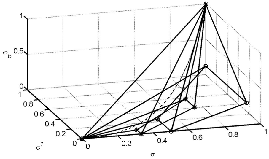
The scheduling parameter ${\sigma }_0\in [0,1]$ and $D_{max}=10$ . Figure 2 shows the convex polyhedron construction result in three-dimensional linear space with $\sigma \in [0,1]$ and division number $\mathrm{d}=2$ . The curve $\mathrm{\Gamma }$ is shown in dash and dot line; the edges of the polyhedron constructed by the method proposed in Azuma et al. ²⁸ are drawn in solid line and the vertex set is marked with a circle; then, the edges of the polyhedron constructed by the given approach are drawn in solid line and the vertex set is marked with a star. Figure 3 shows the volume change of different constructed convex polyhedrons; the method in Azuma et al. ²⁸ is drawn in solid line and the given method in dashed line. Figure 4 shows the analysis result of H_∞ performance using given convex polyhedron construction method and the method proposed in Azuma et al. ²⁸ with PLF, while the parameter curve division number changed from 1 to 25 and the degrees of polynomial PLF are 2 and 3, respectively. The 2- and 3-degree polynomial PLF analysis results are drawn in solid line and dashed line, respectively, where the given method analysis results are marked with triangles and the results from Azuma et al. ²⁸ are marked with stars.

Figure 2.

The construction of convex polyhedron.

Figure 3.

Volume comparison of constructed convex polyhedron.

Figure 4.

The H_∞ performance analysis with different methods and degrees of LPF.

From Figures 2 and 3, it can be seen that the given convex polyhedron construction method more tightly surrounds the parameter curve $\mathrm{\Gamma }$ than the method in Azuma et al. ²⁸ and that means less conservativeness and high accuracy result in following control system analysis and synthesis. From Figure 4, it can be seen that an increase in both the degree of PLF and parameter curve division number can lead to more accurate and less conservative result on closed-loop H_∞ gain analysis, but the computation workload increases rapidly with it. Moreover, the improved construction method achieves better computation efficiency and accuracy than the method given in Azuma et al. ²⁸

Controller synthesis simulation

In this simulation, a turbofan engine PLPV model achieved by Jacobian method which choosing fan relative perturbation speed $\Delta n_L$ as the variable parameter.^30,31 The model state is $x_p=(\Delta n_H,\Delta n_L{)}^T$ , $\Delta n_H$ representing the relative perturbation of high pressure rotor; $u=(\Delta m_f,\Delta A_8{)}^T$ is the control input, which represents the relative perturbation of combustor fuel flow and the nozzle throat area respectively; $y_p=(\Delta n_L,\Delta T_{51}{)}^T$ is the output and $\Delta T_{51}$ stands for relative perturbation of high pressure turbine exit temperature. In simulation, two typical operating conditions are given, altitude $\mathrm{Al}=8.0\mathrm{km}$ , Mach number Ma=0.9 and $\mathrm{Al}=11.0\mathrm{km}$ , Ma=0.9, both with $\Delta n_L\in [0.82,0.98]$ ; the degree of PLPV model and PLF are both chosen as 3; then the convex polyhedron H is constructed by using the parameter curve division number 3 and 5 for two operating conditions in 6 dimensions linear space. Moreover, the controller K(n _L ) is achieved by solving convex optimization problems.

In simulation, eight accuracy turbofan engine linear models are selected by dividing the range of $\Delta n_L\in [0.82,0.98]$ evenly into eight parts under the operating conditions. Then, the unit step responses of these models are simulated using the designed controllers. Figures 5 and 6 show the unit step responses for operating condition 1; Figures 7 and 8 show the unit step responses for operating condition 2.

Figure 5.

Step responses of operating condition 1 at $w_{n_L}=1,w_{T_{51}}=0$ .

Figure 6.

Step responses of operating condition 1 at $w_{n_L}=0,w_{T_{51}}=1$ .

Figure 7.

Step responses of operating condition 2 at $w_{n_L}=1,w_{T_{51}}=0$ .

Figure 8.

Step responses of operating condition 2 at $w_{n_L}=0,w_{T_{51}}=1$ .

As can be seen in Figures 5–8, the control system is stable and shows considerable dynamic response under scheduling of variable parameter. The settling time of unit step responses is less than 2.5 s and the overshoot is less than 0.3%, so the coupling effect between different control channels is weaker and attenuates fast. Moreover, for simulations with other typical operating conditions, the controller design method shows satisfying dynamic performance (settling time < 3.0 s, overshoot < 1.5%), global characteristics, and object adaptability.

Conclusion

A output feedback controller design method for PLPV model with bounded parameter variation rate is given. By combining PLF, sufficient conditions for controller satisfying H_∞ performance are proposed. To resolve the global controller design, this optimization problem is transformed into a new form with decoupling of PLF and full rank controller first. Second, the controller optimization problem is reduced to a normal convex optimization problem with LMIs’ constraint based on the new convex polyhedron construction method using the characteristics of polynomial parameter domain. Then, the simulations on analysis and synthesis of control systems show satisfying control performance in the range of scheduling parameter. Thus, the feasibility and effectiveness of this controller design method are verified.