Sage Journals: Discover world-class research

Abstract

This work extends the application of the finite volume method to predict the acoustic performance of the water muffler with the consideration of elastic walls. The three-dimensional time-domain finite volume method and the improved time-domain impulse method are employed to predict the acoustic attenuation characteristics of mufflers. The present results agree well with analytical solutions and numerical results obtained by finite element method with commercial codes. The effects of different thicknesses of elastic end cavity wall, elastic tube, and cavity walls on acoustic characteristics of a water-filled Helmholtz resonator are investigated. An attempt to simplify the present method with the effective sound speed has been implemented and discussed.

Keywords

Water muffler structural acoustic interaction finite volume method transmission loss elastic wall

Introduction

Pumps are widely used in different industries and are the main sources of noise in piping systems. The vibration and noise induced by the pump operation process will affect the precision of the system control and the normal work functions of downstream equipment.^1,2 Meanwhile, the rapid development of the ship industries has placed stricter requirements of noise control. The water muffler can be used to control the noise of pipeline.³

Accurate prediction of the transmission loss (TL) is important for a well-designed muffler. For the air muffler, there are many mature theories for the prediction of TL with satisfied accuracy, such as the transfer matrix method,⁴ the analytical method,⁵ the finite element method (FEM),⁶ and the boundary element method (BEM).^5,7 In contrast, few references have discussed the acoustic performance of the water muffler. Some efforts^2,8 have been devoted to researching the water muffler in recent years. Since the fluid speed in the pipeline is usually much slower than the sound speed, the fluid flow is usually ignored in published numerical researches. The major difference between the water muffler and the air muffler is the working medium. The interaction between the water and the structure is much stronger than that between the air and the structure. So the theories for the air muffler may not be suitable for the water muffler. Norris and Wickham⁹ described a general theory based on asymptotic methods for acoustical scattering from the elastic water Helmholtz resonator. The results indicated that the wall compliance reduced the resonance frequency in comparison with an identically shaped rigid cavity. Zhou et al.⁸ discussed the effect of the elastic walls on the acoustic characteristics of a water Helmholtz resonator. However, it is hard to use the method in Zhou et al.’s study⁸ to consider the effects of the elastic side-branch tube and main pipe on the acoustic performance.

There are mainly two alternative numerical methods for acoustic problems, the frequency-domain method and the time-domain method. Combining with the frequency domain method, the FEM,⁶ the BEM,⁷ and the finite volume method (FVM)¹⁰ have been applied to analyze the acoustic performance of the muffler. The FEM and the BEM are much more popular than the FVM in frequency domain, due to the wide application of some commercial codes in design. Combining with the time-domain method, the finite difference method (FDM)¹¹ and the FVM¹² have been applied to the acoustic problems. In comparison with the frequency-domain method, the time-domain method has the following advantages: it is easy to carry out, one computation can provide the information of entire frequency band, and the computer memory requirements are not as large as those of the frequency-domain method. So the time-domain method may be more appropriate for the problem with intensive computation and complicate geometry.

The FVM is the most popular numerical method in computational fluid dynamic (CFD) problems. It has been demonstrated to be a reliable approach for the structural,^13–16 acoustic,¹² and structural acoustic¹⁷ problems in recent years. The development of the FVM in the acoustic field is helpful for the application of a unified FVM¹⁸ for fluid-structure-acoustic coupling problems. Xuan et al.¹⁹ presented a time-domain FVM to predict the TL of the air muffler. Then, this method was extended to predict the TL of the air muffler including thermal effects with non-uniform sound speed and density from the commercial code Fluent.¹² Xuan et al.¹⁷ also employed this time-domain FVM to predict the transient response and natural characteristics of structural acoustic coupling systems. This article is going to further extend the application of the time-domain FVM to the acoustic problem of the water muffler with elastic walls. For comparison, the commercial code Comsol is used to solve the same problem.

Basic theory

Mathematical models

According to Newton’s second law, the structural dynamic equation is

\int_{Ω s} ρ_{s} \overset{\cdot\cdot}{u} d Ω = \int_{Ω s} \nabla \cdot σ d Ω + \int_{Ω s} F d Ω

(1)

where Ωs is the structural sub-domain, ρ_s is the solid density, $\overset{\cdot\cdot}{u} = ({\overset{\cdot\cdot}{u}}_{x}, {\overset{\cdot\cdot}{u}}_{y}, {\overset{\cdot\cdot}{u}}_{z})$ is the acceleration vector, σ is the Cauchy stress tensor, and F is the body force which is omitted in the following equations. The subscript s denotes the variable in the structural sub-domain.

The constitutive equations for the three-dimensional linear elastic body is

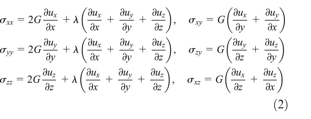
\begin{matrix} σ_{xx} = 2 G \frac{\partial u_{x}}{\partial x} + λ (\frac{\partial u_{x}}{\partial x} + \frac{\partial u_{y}}{\partial y} + \frac{\partial u_{z}}{\partial z}), σ_{xy} = G (\frac{\partial u_{x}}{\partial y} + \frac{\partial u_{y}}{\partial x}) \\ σ_{yy} = 2 G \frac{\partial u_{y}}{\partial y} + λ (\frac{\partial u_{x}}{\partial x} + \frac{\partial u_{y}}{\partial y} + \frac{\partial u_{z}}{\partial z}), σ_{zy} = G (\frac{\partial u_{y}}{\partial z} + \frac{\partial u_{z}}{\partial y}) \\ σ_{zz} = 2 G \frac{\partial u_{z}}{\partial z} + λ (\frac{\partial u_{x}}{\partial x} + \frac{\partial u_{y}}{\partial y} + \frac{\partial u_{z}}{\partial z}), σ_{xz} = G (\frac{\partial u_{x}}{\partial z} + \frac{\partial u_{z}}{\partial x}) \end{matrix}

(2)

where λ and G are the Lamé constants as λ=Eν/[(1+ν)(1 − 2ν)], G = E/[2(1 + ν)]. E is Young’s modulus and ν is Poisson’s ratio.

In structural sub-domain, the free-surface condition and the clamped boundary condition are employed, which can be expressed as

{(σ \cdot n)}_{Γ_{N}} = 0

(3)

{(u)}_{Γ_{C}} = 0

(4)

where u = (u_x, u_y, u_z) denotes the displacement vector, Γ_N is the free-surface, and Γ_C is the clamped surface.

The acoustic wave equation in heterogeneous media is²⁰

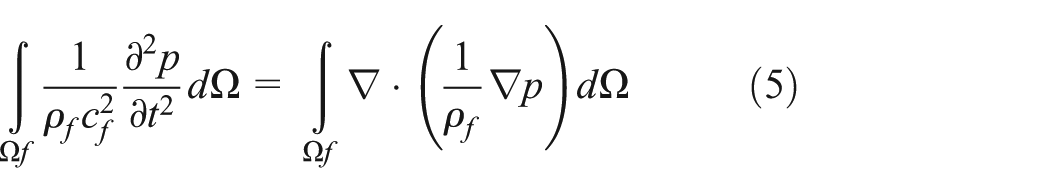
\int_{Ω f} \frac{1}{ρ_{f} c_{f}^{2}} \frac{\partial^{2} p}{\partial t^{2}} d Ω = \int_{Ω f} \nabla \cdot (\frac{1}{ρ_{f}} \nabla p) d Ω

(5)

where Ωf is the acoustic sub-domain, p is the acoustic pressure, ρ_f is the fluid density, and c_f is the acoustic wave speed. The subscript f denotes the variable in the acoustic sub-domain. Equation (5) is suitable for the problem with variable fluid density and acoustic wave speed.

In acoustic sub-domain, two types of boundary conditions are employed. One is the total-reflecting boundary condition, which can be expressed as $\partial p / \partial n = 0$ . The other one is the absorbing boundary condition, which can be expressed as

\frac{1}{c} \frac{\partial p}{\partial t} + \frac{\partial p}{\partial n} = 0

(6)

The interaction boundary conditions between the acoustic and structural sub-domains are

\begin{matrix} - p n = σ \cdot n \\ - \nabla p / ρ_{f} = \overset{\cdot\cdot}{u} \end{matrix}

(7)

The structural and acoustic governing equations are discretized by the time-domain FVM. The formulations and algorithms for the structural acoustic coupling can be found in Xuan et al.¹⁷

Time-domain method for prediction of the muffler’s TL

The muffler’s TL⁴ can be expressed as

TL = 20 \log [{(\frac{A_{i}}{A_{0}})}^{1 / 2} | \frac{p_{in}}{p_{tr}} |]

(8)

where p_in and p_tr are the pressure of the incident wave and the transmitted wave in the frequency domain, respectively; A_i and A_o are the cross-sectional areas of the inlet and the outlet, respectively.

Since the structural acoustic coupling systems are solved by the time-domain FVM, the modified impulse method¹² belonging to the time-domain one is employed. p_in and p_tr can be obtained from their transient expressions by the fast Fourier transform (FFT).

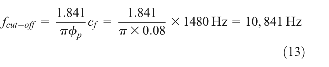
Take the muffler in Figure 1, for example, to explain how the modified impulse method obtains p_in and p_tr in the time domain briefly. Step 1: in the fluid sub-domain, a Gaussian pressure pulse p = exp [−(t − 3T′)²/(T′)²] is applied at the inlet and the absorbing boundary condition is applied at the outlet. Step 2: after a given time 6T′, the inlet is set to be the absorbing boundary, where 6T′ is the minimum time to get a complete Gaussian pressure pulse. So the length l_in of the inlet tube is required to be long enough to make sure that the reflected wave has not reached the inlet within 6T′. In other words, 2 l_in > 6 c_max T′, where c_max is the maximum sound speed at the inlet tube. The maximum effective frequency $f'$ of the given Gaussian pulse should be larger than the maximum predicting frequency of the water muffler. The maximum effective frequency $f'$ is equal to 1/(2T′). Step 3: the given Gaussian pulse can be recorded and considered as p_in. From the simulation, the pressure downstream with plane waves, like the one at point 2 in Figure 1, is recorded and considered as p_tr.

Figure 1.

Geometry of the Helmholtz resonator, namely, Case A.

It has to be noted that if the elasticity of the muffler wall is considered, the fluid–solid interface is set to be interaction boundary; otherwise, the muffler wall is set to be the total-reflecting boundary.

Results and discussion

The effects of elastic tube and cavity walls on the acoustic characteristics of a water-filled Helmholtz resonator are investigated. The geometry of the pipe-mounted Helmholtz resonator considered in this study is shown in Figure 1. The material of resonator is steel with density ρ_s = 7800 kg/m³, Young’s modulus E = 2.16 × 10¹¹ Pa, Poisson’s ratio ν = 0.3, and longitudinal wave speed c_p ≈ 6106 m/s. The fluid medium in the resonator is water with density ρ_f = 1000 kg/m³ and sound speed c_f = 1480 m/s. In order to obtain TL by the modified impulse method, a Gaussian pressure pulse p = exp [−(t − 3/(1.6 × 10⁴))²/(1/(1.6 × 10⁴))²] Pa is applied at the inlet of the main pipe in the fluid sub-domain, where T′ = 1/(1.6 × 10⁴) s is obtained according to 2 l_in > 6 c_max T′ with l_in = 0.3 m and c_max = c_f.

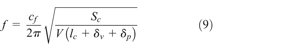
Based on the plane wave theory, the resonance frequency using the low-frequency approximation can be expressed as

f = \frac{c_{f}}{2 π} \sqrt{\frac{S_{c}}{V (l_{c} + δ_{v} + δ_{p})}}

(9)

where $V = π a_{v}^{2} l_{v}$ is the volume of the resonance cavity, $S_{c} = π a_{c}^{2}$ is the cross-sectional area of the neck, l_c is the length of the neck, δ_v and δ_p are the acoustic length correction factors corresponding to the cavity volume and main duct interfaces, respectively. δ_v and δ_p can be expressed as^21,22

δ_{v} = 0.82 a_{c} (1 - 1.33 \frac{a_{c}}{a_{v}})

(10)

δ_{p} = {\begin{matrix} a_{c} [0.8216 - 0.0644 \frac{a_{c}}{a_{p}} - 0.694 {(\frac{a_{c}}{a_{p}})}^{2}], & \frac{a_{c}}{a_{p}} \leq 0.4 \\ a_{c} (0.9326 - 0.6196 \frac{a_{c}}{a_{p}}), & \frac{a_{c}}{a_{p}} > 0.4 \end{matrix}

(11)

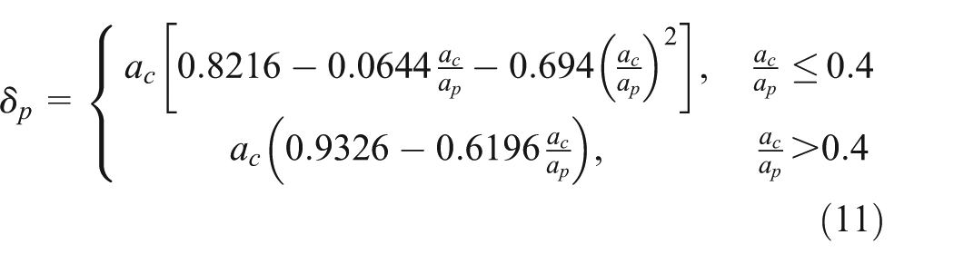
where a_c, a_v, and a_p are the radii of the neck, the cavity, and the main pipe, respectively.

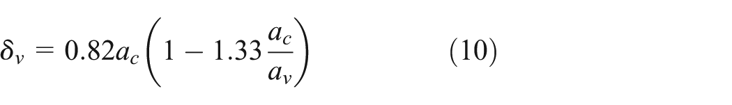
For the Helmholtz resonator (see Figure 1), the length correction factors are δ_v = 0.01 m and δ_p = 0.0114 m from equations (10) and (11), while the acoustic length is

l'_{c} = l_{c} + δ_{v} + δ_{p} = 0.1084 m

(12)

Then, the resonance frequency can be predicted according to equation (9) as f = 340 Hz.

The acoustic performance of resonators, including Case A (see Figure 1) and Cases B–E (see Figure 2), with different conditions is discussed. Table 1 shows the detailed computational information of cases. Since there are few references discussing the acoustic performance of the water muffler, some commercial codes have been used for validation.

Figure 2.

Geometries of different cases: (a) Case B, (b) Case C, (c) Case D, and (d) Case E.

Table 1.

Computational information of different cases.

		FVM			Comsol
		Number of grids (structure)	Number of grids (fluid)	Time step Δt (s)	Number of grids (structure)	Number of grids (fluid)
Case A		–	8544	3 × 10⁻⁶	–	7364
Case B	Case B1 (d = 20 mm)	22,917	31,421	2.5 × 10⁻⁷	7192	39,224
	Case B2 (d = 10 mm)	9614	31,421	3.0 × 10⁻⁷	1751	48,014
	Case B3 (d = 5 mm)	6089	31,627	2.5 × 10⁻⁷	5220	40,357
Case C (d = 10 mm)		168,047	96,718	2.0 × 10⁻⁷	12,255	39,503
Case D (d = 10 mm)		180,760	101,774	2.0 × 10⁻⁷	17,070	41,082
Case E (d = 10 mm)		171,027	393,075	2.5 × 10⁻⁷	29,405	38,161

FVM: finite volume method.

TL without elastic wall (Case A)

The acoustic performance of the resonator without elastic wall is investigated. The cut-off frequency of the main pipe is

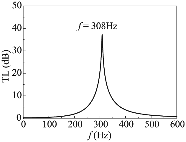
f_{cut - off} = \frac{1.841}{π ϕ_{p}} c_{f} = \frac{1.841}{π \times 0.08} \times 1480 Hz = 10, 841 Hz

(13)

The time step Δt is 3 × 10⁻⁶ s and the sampling time is 0.786432 s, namely, 2¹⁸ sample number (time steps). Time responses at points 1 and 2 (see Figure 1) and TL of the Helmholtz resonator without elastic wall are shown in Figures 3 and 4, respectively. The resonance frequency obtained from different methods is listed in Table 2. The mesh adopted by the present FVM is the same as the one by the commercial code Sysnoise, but it is different from that by the commercial code Comsol. Both Sysnoise and Comsol are FEM codes. The FVM result is in accordance with the Sysnoise result, and there exists little difference between results of FVM and Comsol. The relative error among the results of FVM, equivalent lumped method,⁸ Sysnoise, and Comsol is no more than 2.1%. From Table 2, it is found that Comsol gives more accurate result compared to Sysnoise. So in the following parts, only Comsol is applied for comparison.

Figure 3.

Time responses at points 1 and 2.

Figure 4.

TL of the Helmholtz resonator.

Table 2.

Resonance frequency of the Helmholtz resonator.

	Equation (9)	Zhou et al.⁸	FVM	Sysnoise	Comsol
Resonance frequency (Hz)	340	340 (0.00%)	333 (−2.06%)	333 (−2.06%)	336 (−1.18%)

FVM: finite volume method.

The content in parentheses is the relative error compared to result from equation (9).

Effect of the thickness of the elastic end cavity wall (Case B)

The acoustic performance of the resonator with different thicknesses of elastic end cavity wall is investigated. The sampling time contains 2²⁰ time steps. The mesh employed by the FVM contains two layers of grids along the thickness direction. Cases B1–B3 with different end wall thicknesses are considered. The circumference of the end wall is clamped.

Time responses at point 2 for different cases are shown in Figure 5. At first, the acoustic pressure at point 2 is mainly influenced by the inlet signal, so the curves of different cases show little difference. After some time, the difference begins to manifest and becomes more and more obvious. It is caused by the sound excited by the vibration of the elastic end cavity wall. The time response changes with the variation of the end wall thickness.

Figure 5.

Time responses at point 2.

TL of the Helmholtz resonator with different thicknesses of the end wall is shown in Figure 6. The obtained resonance frequencies are listed in Table 3. The error between the results of the present FVM and Comsol is no more than 0.90% which demonstrates the capability of the FVM for the water muffler with elastic walls. As the end wall thickness decreases, the resonance frequency of the Helmholtz resonator reduces since the interaction between the structure and the water strengthens. Therefore, controlling the end wall thickness can be regarded as an alternative way to design a water muffler for a particular frequency. But when the thickness increases to some certain value, the resonance frequency of the Helmholtz resonator with elastic wall is close to the one with rigid wall according to the comparison between Case A and Case B1. So the scope of the adjustment is limited.

Figure 6.

Influence of the end cavity wall thickness.

Table 3.

Resonance frequency of the Helmholtz resonator with different end wall thicknesses.

Cases	Case A	Case B1	Case B2	Case B3
Comsol (Hz)	336	332	316	237
FVM (Hz)	333	329	318	237
Relative error	−0.89%	−0.90%	0.63%	0.00%

FVM: finite volume method.

Effect of elastic cavity walls

The acoustic performance of the resonator with consideration of various elastic cavity walls is analyzed. The thickness d of the elastic wall is 10 mm. The sampling time also contains 2²⁰ time steps. In Case C, the elasticity of the cavity wall is considered and the cross section between the cavity and the side-branch is clamped. In Case D, the elasticity of the cavity and the side-branch tube is considered and the cross section between the side-branch tube and the main pipe is clamped. In Case E, the elasticity of the cavity, the side-branch tube, and the main pipe are considered and both ends of the main pipe are clamped.

Contours of acoustic pressure (Pa) at different time levels for Case E are shown in Figure 7. It can be seen that the Gaussian impulse applied at the inlet transmits along the main pipe; when the wave arrives the side-branch tube, one part transmits along the side-branch tube to the cavity, another part transmits along the main pipe to the outlet without reflecting wave, and the rest part reflects at the side-branch tube to the inlet with absorbing boundary condition. The wave into the cavity oscillates and transmits to the inlet and outlet until the acoustic pressure decreases close to zero.

Figure 7.

Contours of acoustic pressure (Pa) at different time levels for Case E.

The deformation and contours of displacement u_x at different time levels for Case E are shown in Figure 8. The structure deformation is shown obviously by expanding the displacement 1 × 10¹⁰ times. It can be seen that the deformation is caused by the acoustic pressure acting on the structure via the interface, since there is no other excitation on the structure. No deformation exists at both ends of the pipe for they are clamped. From Figures 7 and 8, it can be observed that the maximum deformation along the radial direction exists at the place with the maximum acoustic pressure. The maximum deformation propagates slower than the axial displacement since the acoustic wave speed is slower compared to the stress wave speed.

Figure 8.

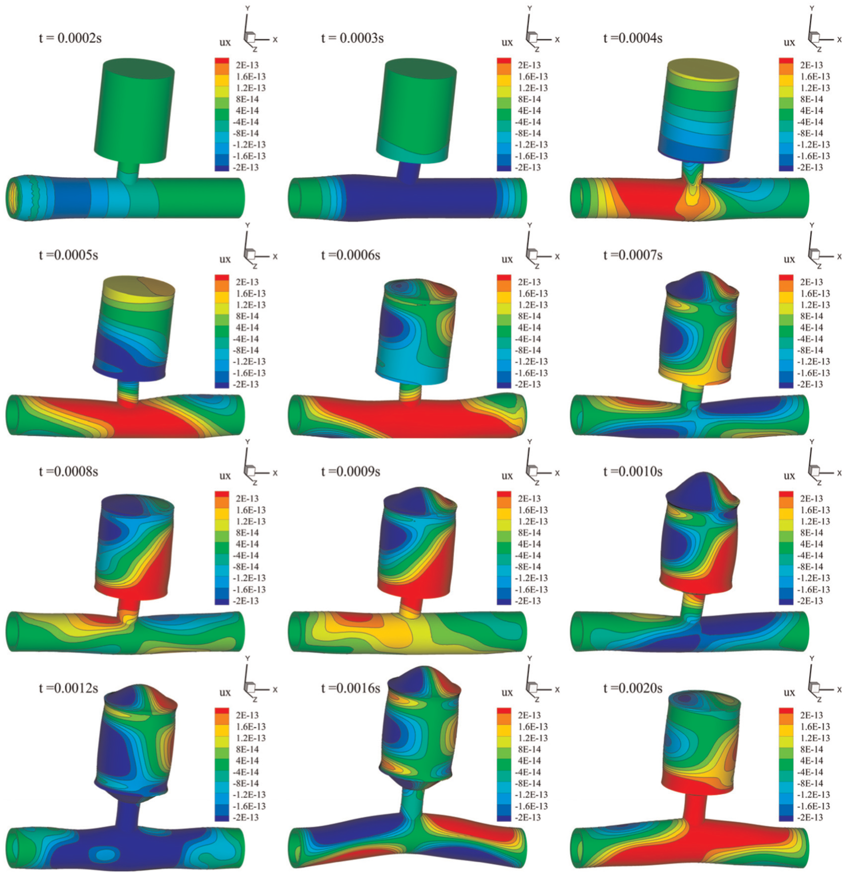
Deformation at different time levels for Case E.

TL of the Helmholtz resonator with the consideration of the structure elasticity is shown in Figure 9. The obtained resonance frequencies are listed in Table 4. When the number of grids is more than 90,000, Comsol could not work, while the present FVM still worked stably. It may be due to huge memory required by Comsol. The relative error between the results of the FVM and Comsol is no more than 4.56% for Cases C–E. The difference may be caused using different meshes.

Figure 9.

TL of the Helmholtz resonator with the consideration of structural elasticity.

Table 4.

Resonance frequencies (Hz) of the Helmholtz resonator for different cases.

	Case C	Case D	Case E
Comsol (Hz)	263	265	263
FVM (Hz)	271	272	275
Relative error	3.04%	2.64%	4.56%

FVM: finite volume method.

Comparing Tables 3 and 4, the resonance frequency of Case B1 is much larger than those of Cases C–E, but the difference among those of Cases C–E is small. The elasticity of the whole cavity wall leads to a significant reduction of not only the end cavity wall but also the resonance frequency. However, the consideration of elastic side-branch tube and main pipe shows little influence on the resonance frequency of the Helmholtz resonator with an elastic cavity.

Attempt to simplify the prediction

In this section, equation (14) from Zhang et al.²³ is employed for the attempt of simplifying the prediction of the resonator’s acoustic performance. The effective sound speed with the consideration of the tube’s elasticity and the fluid’s compressibility is

c_{f} = \sqrt{\frac{K_{f}}{ρ_{f}} {(1 + \frac{D K_{f}}{E δ})}^{- 1}}

(14)

where D is the diameter of the pipe, δ is the pipe wall thickness, and K_f = 2.19 × 10⁹ Pa is the fluid bulk modulus.

Since the present FVM is suitable for heterogeneous media as mentioned, the obtained varying sound speed from equation (14) can be taken directly into account in the solution of acoustic wave equation (5). The simulation of Case A with the effective sound speed is implemented trying to simplify the solving process of Case E. The contour of the varying sound speed from equation (14) is shown in Figure 10. The calculated TL of the Helmholtz resonator is shown in Figure 11. The obtained resonance frequency is smaller than that of Case A, while much larger than that of Case E with the same pipe wall thickness. It indicates that the assumption of the sound speed in Zhang et al.,²³ which aims at the structural acoustic interaction problem in the fluid-conveying pipe, cannot be applied to the acoustic problem in the resonator directly. The reason may be equation (14) is not suitable for the resonator’s cavity and the neck, which is not long enough. The attempt to simplify the prediction of the TL of the resonator is not successful.

Figure 10.

The distribution of sound speed in the Helmholtz resonator.

Figure 11.

TL of the Helmholtz resonator with heterogeneous sound speed.

Conclusion

In this study, the time-domain FVM is applied to predict the acoustic performance of the water muffler with the consideration of elastic walls. The modified impulse method is employed to predict the acoustic performance of the Helmholtz resonator.

The acoustic performance of the Helmholtz resonator without elastic wall is predicted. The present FVM results agree well with those from the equivalent lumped method and commercial codes Sysnoise and Comsol. Then, the acoustic performance of the resonator with different thicknesses of the elastic end cavity wall is investigated. The present FVM results agree well with those from Comsol. The elasticity of the end cavity wall leads to a reduction of the resonance frequency, which decreases with the decrement of the end wall thickness. The effects of elastic tube and cavity walls on acoustic characteristics of the Helmholtz resonator are also investigated. The consideration of the whole elastic cavity wall causes the resonance frequency to reduce significantly, while consideration of the elastic side-branch tube and main pipe shows little influence on the resonance frequency of the Helmholtz resonator with an elastic cavity.

The effective sound speed with the consideration of the tube’s elasticity and the fluid’s compressibility is employed trying to simplify the simulation by avoiding the solution of the structural dynamic equation. Unfortunately, the obtained results are not satisfied which demonstrates that the simplification is not reasonable.

Footnotes

Academic Editor: Roslinda Nazar

Declaration of conflicting interests

The author(s) declared no potential conflicts of interest with respect to the research, authorship, and/or publication of this article.

Funding

The author(s) disclosed receipt of the following financial support for the research, authorship, and/or publication of this article: This work was supported by the National Natural Science Foundation of China (no. 51509232). Their financial support is gratefully acknowledged.

References

Rzentkowski

Zbroja

Experimental characterization of centrifugal pumps as an acoustic source at the blade-passing frequency. J Fluid Struct 2000; 14: 529–558.

Liu

. Acoustic performance of a water muffler. Noise Control Eng J 2015; 63: 239–248.

Cheng

Zhang

Liu

. The liquid-born noise and its control in water pipelines of ships. Noise Vib Control 2003; 24: 31–34.

Munjal

ML.

Acoustics of ducts and mufflers. New York: Wiley Interscience, 1987.

Selamet

ZL.

Acoustic attenuation performance of circular expansion chambers with extended inlet/outlet. J Sound Vib 1999; 223: 197–212.

Mehdizadeh

Paraschivoiu

A three-dimensional finite element approach for predicting the transmission loss in mufflers and silencers with no mean flow. Appl Acoust 2005; 66: 902–918.

Zhang

Cheng

CRY

. Boundary element analysis of mufflers with an improved method for deriving the four-pole parameters. J Sound Vib 1998; 217: 767–779.

Zhou

Liu

. Effect of elastic cavity walls on acoustic characteristics of a water-filled Helmholtz resonator: equivalent lumped parameter model for cylindrical cavity. Acta Acust 2007; 32: 426–434.

Norris

Wickham

Elastic Helmholtz resonators. J Acoust Soc Am 1993; 93: 617–630.

10.

Torregrosa

Broatch

Gil

. Analysis of acoustic networks including cavities by means of a linear finite volume method. J Sound Vib 2012; 331: 4575–4586.

11.

Broatch

Serrano

Moya

Time-domain computation of muffler frequency response: comparison of different numerical schemes. J Sound Vib 2007; 305: 333–347.

12.

Xuan

Gong

Ming

. A time-domain finite volume approach for prediction of muffler transmission loss including thermal effects. Proc IMechE, Part C: J Mechanical Engineering Science 2013; 228: 108–118.

13.

Demirdžić

Martinović

Finite volume method for thermo-elasto-plastic stress analysis. Comput Method Appl M 1993; 109: 331–349.

14.

Wheel

MA.

A geometrically versatile finite volume formulation for plane elastostatic stress analysis. J Strain Anal Eng 1996; 31: 111–116.

15.

Slone

Bailey

Cross

Dynamic solid mechanics using finite volume methods. Appl Math Model 2003; 27: 69–87.

16.

Xuan

Ming

Gong

. A finite volume time domain method for in-plane vibration on mixed grids. J Vib Acoust 2013; 136: 0110031–0110039.

17.

Xuan

Jin

Gong

. Time domain finite volume method for three-dimensional structural–acoustic coupling analysis. Appl Acoust 2014; 76: 138–149.

18.

Maneeratana

Development of the finite volume method for non-linear structural applications. London: University of London, 2000.

19.

Xuan

Zhang

Ming

. Unstructured finite volume time domain method for prediction of muffler’s acoustic attenuation performance. J Harbin Eng Univ 2012; 33: 185–191.

20.

Bergmann

PG.

The wave equation in a medium with a variable index of refraction. J Acoust Soc Am 1946; 17: 329–333.

21.

Selamet

ZL.

Circular asymmetric Helmholtz resonators. J Acoust Soc Am 2000; 107: 2360–2369.

22.

ZL.

Acoustic length correction of closed cylindrical side-branched tube. J Sound Vib 2005; 283: 1180–1186.

23.

Zhang

Huang

Tijsseling

AS.

Review of FSI analysis of fluid-conveying pipes. J Hydrodyn 2000; 15: 366–379.

A time-domain finite volume method for the prediction of water muffler transmission loss considering elastic walls

Abstract

Keywords

Introduction

Basic theory

Mathematical models

Time-domain method for prediction of the muffler’s TL

Results and discussion

TL without elastic wall (Case A)

Effect of the thickness of the elastic end cavity wall (Case B)

Effect of elastic cavity walls

Attempt to simplify the prediction

Conclusion

Footnotes

Declaration of conflicting interests

Funding

References