On solving fractional mobile/immobile equation

Abstract

In this article, a numerical efficient method for fractional mobile/immobile equation is developed. The presented numerical technique is based on the compact finite difference method. The spatial and temporal derivatives are approximated based on two difference schemes of orders $O({\tau }^{2-\alpha })$ and $O(h^4)$ , respectively. The proposed method is unconditionally stable and the convergence is analyzed within Fourier analysis. Furthermore, the solvability of the compact finite difference approach is proved. The obtained results show the ability of the compact finite difference.

Introduction

The governing equation of transport was derived based on Fick’s law and is commonly called the advection-dispersion equation (ADE). ¹ The ADE will predict a breakthrough curve (BTC) that can be described by a Gaussian distribution function from an instantaneously releasing solute source. ¹ The interested readers can find more details in previous studies.^2–7 Also, the mobile/immobile model is considered in previous studies.^8–12

Here, the time fractional mobile/immobile equation is studied to the following form^12,13

$$\begin{array}{l}\frac{\partial u(x,t)}{\partial t}+\frac{{\partial }^{\alpha }u(x,t)}{\partial t^{\alpha }}=\frac{{\partial }^{2}u(x,t)}{\partial x^2}-\frac{\partial u(x,t)}{\partial x}\\ +f(x,t),(x,T)\in [0h]\times [0T],0<\alpha <1\end{array}$$

(1)

when the boundary conditions are

$$\begin{array}{c}u(0,t)={\varphi }_1(t)\hfill \\ 0<t<T\hfill \\ \multicolumn{1}{c}{u(h,t)={\varphi }_2(t)}\end{array}$$

(2)

and the initial condition is

$$u(x,0)=g(x),0<x<h$$

(3)

where ${\partial }^{\alpha }(•)/\partial t^{\alpha }$ is the Caputo fractional derivative of order $0<\alpha <1$ . For getting more information on fractional PDEs the interested readers can refer to.^21–25

Some numerical methods have been developed for the solution of equation (1) such as finite difference (FD) method^12,13 and meshless method. ¹⁴ Also, the fractional equation is studied by several methods, for example, high-order FD scheme for modified anomalous fractional sub-diffusion equation^15,16 and FD method for a class of fractional sub-diffusion equations. ¹⁷

The main aim of this article is to see the performances of the compact FD for the fractional mobile/immobile equation. The article is organized as follows. In section “Compact FD scheme,” we develop a high-order FD scheme. Section “Stability analysis” presents the stability analysis for the proposed difference scheme. In section “Convergence analysis,” the convergence analysis is studied. Some numerical results are presented in section “Numerical results.” Finally, a brief conclusion is written in section “Conclusion.”

Compact FD scheme

Let $h=L/M$ and $\tau =T/N$ be the step sizes of spatial and temporal variables, respectively. So, we can define spatial and temporal nodes as $x_j=\mathrm{jh}$ , for $j=0,1,2,\dots ,M,$ and $t_k=k\tau$ , for $k=0,1,2,\dots ,N.$

The exact and approximate solutions at the point $(x_j,t_k)$ are denoted by $u_j^k$ and $U_j^k$ , respectively. We introduce the following notations

$$\begin{array}{c}{\delta }_x{u}_j^k=\frac{u_{j+1}^k-u_{j-1}^k}{h}\hfill \\ {\delta }_x^2{u}_j^k=\frac{u_{j+1}^k-2u_j^k+u_{j-1}^k}{h^2}\hfill \\ \frac{\partial u_j^k}{\partial t}={\delta }_t{u}_j^k=\frac{u_j^k-u_j^{k-1}}{\tau }+O(\tau )\hfill \end{array}$$

where $u_j^k=u(x_j,t_k)$ .

Lemma 1 ²⁶

Assume the below equation

$$\gamma \frac{d^{2}y(x)}{d{x}^2}-\beta \frac{\mathrm{dy}(x)}{\mathrm{dx}}=f(x),x\in (0,L)$$

(4)

with

$$y(0)=y_0,y(L)=y_L$$

A CFD scheme for it is as follows

$$\begin{array}{l}\left(\gamma +\frac{{\beta }^2{h}^2}{12\gamma }\right){\delta }_x^2{y}_j-\beta {\delta }_x{y}_j=f_j\\ +\frac{h^2}{12}\left({\delta }_x^2{f}_j-\frac{\beta }{\gamma }{\delta }_x{f}_j\right)+O(h^4)\end{array}$$

(5)

Let

$$w(x,t)=\frac{1}{\Gamma (1-\alpha )}\underset{0}{\overset{t}{\int }}\frac{\partial u(x,z)}{\partial z}(t-z{)}^{-\alpha }\mathrm{dz}$$

(6)

so equation (1) can be written as follows

$$-\frac{{\partial }^{2}u(x,t)}{\partial x^2}+\frac{\partial u(x,t)}{\partial x}+\frac{\partial u(x,t)}{\partial t}=f(x,t)-w(x,t)$$

(7)

we can write equation (7) as follows

$$\begin{array}{c}-(1+\frac{h^2}{12}){\delta }_x^2{u}_j^k+{\delta }_x{u}_j^k=(f_j^k-w_j^k-\frac{\partial u_j^k}{\partial t})+(r_1{)}_j^k\hfill \\ +\frac{h^2}{12}({\delta }_x^2(f_j^k-w_j^k-\frac{\partial u_j^k}{\partial t})-{\delta }_x(f_j^k-w_j^k-\frac{\partial u_j^k}{\partial t}))\hfill \end{array}$$

(8)

where there is a constant c₁ such that

$$|(r_1{)}_j^k|\le c_1(h^4)$$

(9)

Based on Lemma 2 in Sun and Wu ¹⁸ we have

$$\begin{array}{c}\multicolumn{1}{c}{W_j^k=\frac{1}{\Gamma (1-\alpha )}\underset{0}{\overset{t_k}{\int }}\frac{\partial u(x_j,t)}{\partial t}(t_k-t{)}^{-\alpha }\mathrm{dt}}\\ =\frac{{\tau }^{-\alpha }}{\Gamma (2-\alpha )}\hfill \\ [b_0{u}_j^k-\sum _{m=1}^{k-1}(b_{k-m-1}-b_{k-m})u_j^m-b_{k-1}{u}_j^0]+(r_2{)}_j^k\hfill \end{array}$$

(10)

where there exists a constant $c_2$ such that

$$|(r_2{)}_j^k|\le c_2({\tau }^{2-\alpha })$$

(11)

Substituting equation (10) into equation (8) gives

$$\begin{array}{c}-(1+\frac{h^2}{12}){\delta }_x^2{u}_j^k+{\delta }_x{u}_j^k=(f_j^k-W_j^k-{\delta }_t{u}_j^k)\hfill \\ +\frac{h^2}{12}({\delta }_x^2(f_j^k-W_j^k-{\delta }_t{u}_j^k)-{\delta }_x(f_j^k-W_j^k-{\delta }_t{u}_j^k))+R_j^k\hfill \end{array}$$

(12)

where

$$\left|R_j^k\right|\le C(\tau +h^4)$$

(13)

Denoting $\mu ={\tau }^{-\alpha }/(\Gamma (2-\alpha ))$ , the proposed difference scheme is

$$A{U}^k=\frac{1}{\tau }B{U}^{k-1}+\mu {\displaystyle \sum _{m=1}^{k-1}(b_{k-m-1}-b_{k-m})}B{U}^m+\mu b_{k-1}B{U}^0+B{F}^k$$

(14)

where

$$\begin{array}{c}\multicolumn{1}{c}{\mathbf{A}=\mathrm{tri}[-\frac{1}{h^2}(1+\frac{h^2}{12})-\frac{1}{2h}+\frac{\mu }{12}+\frac{1}{12\tau }+\frac{h\mu }{24}+\frac{h}{24\tau },\frac{2}{h^2}(1+\frac{h^2}{12})+\frac{5\mu }{6}+\frac{5}{6\tau }}\\ -\frac{1}{h^2}(1+\frac{h^2}{12})+\frac{1}{2h}+\frac{\mu }{12}+\frac{1}{12\tau }-\frac{h\mu }{24}-\frac{h}{24\tau }]\hfill \end{array}$$

$$B=\left[\begin{array}{cccc}\frac{5}{6}\hfill & (\frac{1}{12}-\frac{h}{24})\hfill & \hfill & \hfill \\ \multicolumn{1}{c}{(\frac{1}{12}+\frac{h}{24})}& \ddots \hfill & \ddots \hfill & \hfill \\ \hfill & \ddots \hfill & \ddots \hfill & (\frac{1}{12}-\frac{h}{24})\hfill \\ \hfill & \hfill & (\frac{1}{12}+\frac{h}{24})\hfill & \frac{5}{6}\hfill \end{array}\right]$$

Lemma 2

The matrix A is non-singular.

Proof

For $j=1,2,\dots ,M-1$ , the eigenvalues of A are

$$\begin{array}{l}{\lambda }_j=\left(2{\mu }_1+\frac{5\mu }{6}+\frac{5}{6\tau }\right)+\sqrt{\left[\left(\frac{\mu }{12}-{\mu }_1+\frac{1}{12\tau }\right)+\left(\frac{h\mu }{24}+\frac{h}{24\tau }-\frac{1}{2h}\right)\right]}\\ \times \sqrt{\left[\left(\frac{\mu }{12}-{\mu }_1+\frac{1}{12\tau }\right)-\left(\frac{h\mu }{24}+\frac{h}{24\tau }-\frac{1}{2h}\right)\right]}\cos \left(\frac{j\pi }{M}\right)\end{array}$$

that is

$${\lambda }_j=\left(2{\mu }_1+\frac{5\mu }{6}+\frac{5}{6\tau }\right)+2\sqrt{\left[{\left(\frac{\mu }{12}-{\mu }_1+\frac{1}{12\tau }\right)}^2-{\left(\frac{h\mu }{24}+\frac{h}{24\tau }-\frac{1}{2h}\right)}^2\right]}\cos \left(\frac{j\pi }{M}\right)$$

In case of

$${(\frac{\mu }{12}-{\mu }_1+\frac{1}{12\tau })}^2-{(\frac{h\mu }{24}+\frac{h}{24\tau }-\frac{1}{2h})}^2\le 0$$

the eigenvalues of A can be written as $\lambda =a+\mathrm{bi}$ with non-zero real part $(a\ne 0)$ . For the case

$${(\frac{\mu }{12}-{\mu }_1+\frac{1}{12\tau })}^2-{(\frac{h\mu }{24}+\frac{h}{24\tau }-\frac{1}{2h})}^2>0$$

if $(\mu /12)-{\mu }_1+(1/12\tau )\ge 0$ we have

$$\begin{array}{l}{\lambda }_j\ge 2{\mu }_1+\frac{5\mu }{6}+\frac{5}{6\tau }-2\left(\frac{\mu }{12}-{\mu }_1+\frac{1}{12\tau }\right)\\ =4{\mu }_1+\frac{2\mu }{3}+\frac{2}{3\tau }>0\end{array}$$

and if $(\mu /12)-{\mu }_1+(1/12\tau )<0$

$${\lambda }_j\ge 2{\mu }_1+\frac{5\mu }{6}+\frac{5}{6\tau }+2(\frac{\mu }{12}-{\mu }_1+\frac{1}{12\tau })=\mu +\frac{1}{\tau }>0$$

Since ${\mu }_1,\mu >0$ thus A is non-singular matrix.

Theorem 1

For the appeared scheme in equation (14), there is a unique solution.

Proof

We must solve linear system of equations $A{U}^k=b$ at each $t_k=k\tau$ to obtain the numerical solution. Since for any $\mu$ and ${\mu }_1$ , the coefficient matrix A is invertible so the solution of scheme in equation (14) exists and is unique.

Stability analysis

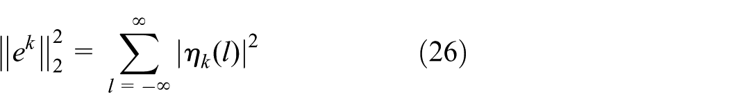
Let ${\tilde{U}}_j^n$ be the approximated solution of equation (14). Consider

$${\rho }_j^k=U_j^k-{\tilde{U}}_j^k,j=0,1,\dots ,M,k=0,1,\dots ,N$$

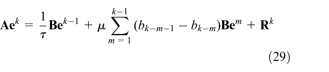
With this definition and regarding equation (14), we can obtain the round-off error equation as

$$\mathbf{A}{\rho }^k=\frac{1}{\tau }\mathbf{B}{\rho }^{k-1}+\mu \sum _{m=1}^{k-1}(b_{k-m-1}-b_{k-m})\mathbf{B}{\rho }^m+\mu b_{k-1}\mathbf{B}{\rho }^0$$

(15)

where

$${\rho }_0^k={\rho }_0^k=0$$

where

$${\rho }^k=[{\rho }_1^k,{\rho }_2^k,\dots ,{\rho }_{M-1}^k]$$

Now we define the grid function ¹⁹

$${\rho }^k(x)=\{\begin{array}{cc}\multicolumn{1}{c}{{\rho }_j^k}& x_j-\frac{h}{2}<x\le x_j+\frac{h}{2}\hfill \\ \multicolumn{1}{c}{0}& 0\le x\le \frac{h}{2}\mathrm{or}L-\frac{h}{2}<x\le L\hfill \end{array}$$

Then ${\rho }^k(x),k=1,2,\dots ,N,$ can be expanded in a Fourier series

$${\rho }^k(x)=\sum _{l=-\infty }^{\infty }{d}_k(l)e^{i2\pi \mathrm{lx}/L}$$

where

$$d_k(l)=\frac{1}{L}\underset{0}{\overset{L}{\int }}{\rho }^k(x)e^{-i2\pi \mathrm{lx}/L}\mathrm{dx}$$

Now introduce the following norm ¹⁹

$$\Vert {\rho }^k{\Vert }_2={\left(\sum _{j=1}^{M-1}h{\left|{\rho }_j^k\right|}^2\right)}^{\frac{1}{2}}={\left[\underset{0}{\overset{L}{\int }}{|{\rho }^k(x)|}^2\mathrm{dx}\right]}^{\frac{1}{2}}$$

Note that we can obtain

$$\Vert {\rho }^k{\Vert }_2^2=\sum _{l=-\infty }^{\infty }{|d_k(l)|}^2$$

(16)

by using Parseval equality

$$\underset{0}{\overset{L}{\int }}{|{\rho }^k(x)|}^2\mathrm{dx}=\sum _{l=-\infty }^{\infty }{|d_k(l)|}^2$$

We can assume the solution of equation (15) as

$${\rho }_j^k=d_k{e}^{i\sigma \mathrm{jh}}$$

where $\sigma =2\pi l/L$ . Now, substituting this expression into equation (15) yields

$$d_k=\frac{(1-\frac{{\sin }^2\frac{\theta }{2}}{3}-\frac{\mathrm{ih}\sin \theta }{12})[\sum _{m=1}^{k-1}\mu (b_{k-m-1}-b_{k-m})d_m+\mu b_{k-1}{d}_0+\frac{1}{\tau }{d}_{k-1}]}{4{\mu }_1{\sin }^2\frac{\theta }{2}+\mu -\frac{\mu }{3}{\sin }^2\frac{\theta }{2}+\frac{1}{\tau }-\frac{1}{3\tau }{\sin }^2\frac{\theta }{2}+\frac{i}{h}\sin \theta -\frac{\mathrm{ih}\mu }{12}\sin \theta -\frac{\mathrm{ih}}{12\tau }\sin \theta }$$

(17)

where

$${\mu }_1=\frac{1}{h^2}(1+\frac{h^2}{12}),\mu =\frac{1}{{\tau }^{\alpha }\Gamma (2-\alpha )}$$

Lemma 3

The below inequality holds

$$\left|\frac{(\mu -\frac{\mu }{3}{\sin }^2\frac{\theta }{2}-\frac{\mathrm{ih}\mu }{12}\sin \theta )+(\frac{1}{\tau }-\frac{1}{3\tau }{\sin }^2\frac{\theta }{2}-\frac{\mathrm{ih}}{12\tau }\sin \theta )}{4{\mu }_1{\sin }^2\frac{\theta }{2}+\mu -\frac{\mu }{3}{\sin }^2\frac{\theta }{2}+\frac{1}{\tau }-\frac{1}{3\tau }{\sin }^2\frac{\theta }{2}+\frac{i}{h}\sin \theta -\frac{\mathrm{ih}\mu }{12}\sin \theta -\frac{\mathrm{ih}}{12\tau }\sin \theta }\right|\le 1$$

(18)

Proof

Because of $h\le 1$ , $\tau \le 1$ , and $\Gamma (2-\alpha )>0$ we can see that $\mu >0$ . Furthermore ${\mu }_1>1$ , too. So, it is easy to see that

$$\begin{array}{c}\frac{8}{3}\mu {\mu }_1\stackrel{2}{\sin }\frac{\theta }{2}-\frac{8\mu {\mu }_1}{3}\stackrel{4}{\sin }\frac{\theta }{2}=\frac{8}{3}\mu {\mu }_1\stackrel{2}{\sin }\frac{\theta }{2}\stackrel{2}{\cos }\frac{\theta }{2}\ge 0\hfill \\ \frac{8{\mu }_1}{3\tau }\stackrel{2}{\sin }\frac{\theta }{2}-\frac{8{\mu }_1}{3\tau }\stackrel{4}{\sin }\frac{\theta }{2}=\frac{8{\mu }_1}{3\tau }\stackrel{2}{\sin }\frac{\theta }{2}\stackrel{2}{\cos }\frac{\theta }{2}\ge 0\hfill \\ \frac{2}{3\tau }{\mu }_1\stackrel{2}{\sin }\frac{\theta }{2}-\frac{2}{3\tau }\stackrel{2}{\sin }\frac{\theta }{2}=\frac{2}{3}\stackrel{2}{\sin }\frac{\theta }{2}({\mu }_1-1)\ge 0\hfill \\ \frac{2}{3}\mu {\mu }_1\stackrel{2}{\sin }\frac{\theta }{2}-\frac{2}{3}\mu \stackrel{2}{\sin }\frac{\theta }{2}=\frac{2}{3}\mu \stackrel{2}{\sin }\frac{\theta }{2}({\mu }_1-1)\ge 0\hfill \end{array}$$

(19)

The relation (18) holds if and only if

$$\begin{array}{c}\multicolumn{1}{c}{0\le {\left(4{\mu }_1{\sin }^2\frac{\theta }{2}\right)}^2+2\left(4{\mu }_1{\sin }^2\frac{\theta }{2}\right)}\\ (\mu -\frac{\mu }{3}{\sin }^2\frac{\theta }{2}+\frac{1}{\tau }-\frac{1}{3\tau }{\sin }^2\frac{\theta }{2})\hfill \\ +\frac{1}{h^2}\stackrel{2}{\sin }\theta -2\left(\frac{1}{h}\sin \theta \right)(\frac{h\mu }{12}\sin \theta +\frac{h}{12\tau }\sin \theta )\hfill \end{array}$$

If we put

$$\begin{array}{c}\frac{\mu }{6}{\sin }^2\theta =\frac{2}{3}\mu {\sin }^2\frac{\theta }{2}-\frac{2}{3}\mu {\sin }^4\frac{\theta }{2}\hfill \\ \frac{1}{6\tau }\stackrel{2}{\sin }\theta =\frac{2}{3\tau }\stackrel{2}{\sin }\frac{\theta }{2}-\frac{2}{3\tau }\stackrel{4}{\sin }\frac{\theta }{2}\hfill \end{array}$$

then relation (18) holds if and only if

$$\begin{array}{c}{\left(4{\mu }_1{\sin }^2\frac{\theta }{2}\right)}^2+(\frac{8}{3}{\mu }_1\mu {\sin }^2\frac{\theta }{2}-\frac{8}{3}{\mu }_1\mu {\sin }^4\frac{\theta }{2})+\frac{14}{3}{\mu }_1\mu \stackrel{2}{\sin }\frac{\theta }{2}\hfill \\ +(\frac{8}{3\tau }{\mu }_1{\sin }^2\frac{\theta }{2}-\frac{8}{3\tau }{\mu }_1{\sin }^4\frac{\theta }{2})+\frac{1}{h^2}\stackrel{2}{\sin }\frac{\theta }{2}+\frac{14}{3\tau }{\mu }_1\stackrel{2}{\sin }\frac{\theta }{2}\hfill \\ +(\frac{2}{3}{\mu }_1\mu {\sin }^2\frac{\theta }{2}-\frac{2}{3}\mu {\sin }^2\frac{\theta }{2})+\frac{2}{3}\mu \stackrel{4}{\sin }\frac{\theta }{2}+\frac{2}{3\tau }\stackrel{4}{\sin }\frac{\theta }{2}\hfill \end{array}$$

which completes the proof.

Theorem 2

Let $d_k$ be the solutions of equation (17), so

$$|d_k|\le |d_0|,k=1,2,\dots ,N$$

(20)

Proof

In case of $k=1$ according to equation (17), we have

$$d_1=\frac{(1-\frac{{\sin }^2\frac{\theta }{2}}{3}-\frac{\mathrm{ih}\sin \theta }{12})(\mu +\frac{1}{\tau })d_0}{4{\mu }_1{\sin }^2\frac{\theta }{2}+\mu -\frac{\mu }{3}{\sin }^2\frac{\theta }{2}+\frac{1}{\tau }-\frac{1}{3\tau }{\sin }^2\frac{\theta }{2}+\frac{i}{h}\sin \theta -\frac{\mathrm{ih}\mu }{12}\sin \theta -\frac{\mathrm{ih}}{12\tau }\sin \theta }$$

or

$$d_1=\frac{(1-\frac{{\sin }^2\frac{\theta }{2}}{3}-\frac{\mathrm{ih}\sin \theta }{12})(\mu +\frac{1}{\tau })d_0}{(4{\mu }_1{\sin }^2\frac{\theta }{2}+\mu (1-\frac{{\sin }^2\frac{\theta }{2}}{3})+\frac{1}{\tau }(1-\frac{{\sin }^2\frac{\theta }{2}}{3}))+i(\frac{\sin \theta }{h}-\frac{h\mu \sin \theta }{12}-\frac{h\sin \theta }{12\tau })}$$

Also, we can write

$$\left|d_1\right|=\frac{\sqrt{{(1-\frac{1}{3}{\sin }^2\frac{\theta }{2})}^2+{\left(\frac{h\sin \theta }{12}\right)}^2}(\mu +\frac{1}{\tau })\left|d_0\right|}{\sqrt{{(4{\mu }_1{\sin }^2\frac{\theta }{2}+\mu (1-\frac{{\sin }^2\frac{\theta }{2}}{3})+\frac{1}{\tau }(1-\frac{{\sin }^2\frac{\theta }{2}}{3}))}^2+{(\frac{\sin \theta }{h}-\frac{h\mu \sin \theta }{12}-\frac{h\sin \theta }{12\tau })}^2}}$$

Now, Lemma 3 yields

$$\left|d_1\right|\le \left|d_0\right|$$

Suppose

$$\left|d_n\right|\le \left|d_0\right|,n=1,2,\dots ,k-1$$

Now, equation (17) yields

$$\left|d_{k-1}\right|\le \frac{|1-\frac{{\sin }^2\frac{\theta }{2}}{3}-\frac{\mathrm{ih}\sin \theta }{12}|(\mu (b_0-b_{k-1})\left|d_0\right|+\mu b_{k-1}\left|d_0\right|+\frac{1}{\tau }\left|d_0\right|)}{|4{\mu }_1{\sin }^2\frac{\theta }{2}+\mu -\frac{\mu }{3}{\sin }^2\frac{\theta }{2}+\frac{1}{\tau }-\frac{1}{3\tau }{\sin }^2\frac{\theta }{2}+\frac{i}{h}\sin \theta -\frac{\mathrm{ih}\mu }{12}\sin \theta -\frac{\mathrm{ih}}{12\tau }\sin \theta |}$$

so

$$\left|d_k\right|\le \left|d_0\right|$$

which completes the proof.

Theorem 3

The CFD scheme (14) is unconditionally stable.

Proof

Using inequality (20) in equation (16) yields

$$\Vert {\rho }^k{\Vert }_2^2=\sum _{l=\infty }^{\infty }{|d_k(l)|}^2\le \sum _{l=\infty }^{\infty }{|d_0(l)|}^2=\Vert {\rho }^0{\Vert }_2^2$$

so we have

$$\Vert {\rho }^k{\Vert }_2\le \Vert {\rho }^0{\Vert }_2$$

Convergence analysis

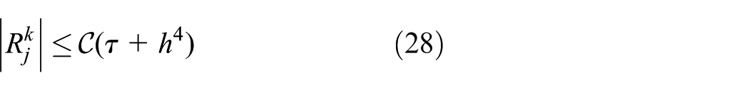
Here, we analyzed the compact difference scheme (14) in terms of convergence. We will show the relation (14) has the spatial accuracy of fourth order. For this end, we need some lemmas and theorems that will be expressed. First, we consider definitions of $e^k(x)$ and $R^k(x)$ in Chen et al. ²⁰ Thus, for $k=0,1,\dots ,N,$ $e^k(x)$ and $R^k(x)$ are

$$\begin{array}{c}{e}^k(x)=\sum _{l=-\infty }^{\infty }{\eta }_k(l)e^{\frac{i2\pi \mathrm{lx}}{L}}\hfill \\ R^k(x)=\sum _{l=-\infty }^{\infty }{\xi }_k(l)e^{\frac{i2\pi \mathrm{lx}}{L}}\hfill \end{array}$$

where

$$\begin{array}{c}{\eta }_k(l)=\frac{1}{L}\underset{0}{\overset{L}{\int }}{e}^k(x)e^{\frac{-i2\pi \mathrm{lx}}{L}}\mathrm{dx}\hfill \\ {\xi }_k(l)=\frac{1}{L}\underset{0}{\overset{L}{\int }}{R}^k(x)e^{\frac{-i2\pi \mathrm{lx}}{L}}\mathrm{dx}\hfill \end{array}$$

Now, we define the following notations ²⁰

$$e_j^k=u(x_j,t_k)-U_j^k$$

(21)

where

$$e^k=[e_1^k,e_2^k,\dots ,e_{M-1}^k],R^k=[R_1^k,R_2^k,\dots ,R_{M-1}^k]$$

and introduce the following norms

$$\Vert e^k{\Vert }_2={\left(\sum _{j=1}^{M-1}h{\left|e_j^k\right|}^2\right)}^{\frac{1}{2}}={\left[\underset{0}{\overset{L}{\int }}{|e^k(x)|}^2\mathrm{dx}\right]}^{\frac{1}{2}}$$

(22)

$$\Vert R^k{\Vert }_2={\left(\sum _{j=1}^{M-1}h{\left|R_j^k\right|}^2\right)}^{\frac{1}{2}}={\left[\underset{0}{\overset{L}{\int }}{|R^k(x)|}^2\mathrm{dx}\right]}^{\frac{1}{2}}$$

(23)

Using the Parseval equality

$$\underset{0}{\overset{L}{\int }}{|e^k(x)|}^2\mathrm{dx}=\sum _{l=-\infty }^{\infty }{|{\eta }_k(l)|}^2$$

(24)

and

$$\underset{0}{\overset{L}{\int }}{|R^k(x)|}^2\mathrm{dx}=\sum _{l=-\infty }^{\infty }{|{\xi }_k(l)|}^2$$

(25)

Also, we have

$$\Vert e^k{\Vert }_2^2=\sum _{l=-\infty }^{\infty }{|{\eta }_k(l)|}^2$$

(26)

$$\Vert R^k{\Vert }_2^2=\sum _{l=-\infty }^{\infty }{|{\xi }_k(l)|}^2$$

(27)

We can obtain

$$\left|R_j^k\right|\le \mathcal{C}(\tau +h^4)$$

(28)

Subtracting equation (14) from equation (12), we obtain

$$\mathbf{A}{\mathbf{e}}^k=\frac{1}{\tau }\mathbf{B}{\mathbf{e}}^{k-1}+\mu \sum _{m=1}^{k-1}(b_{k-m-1}-b_{k-m})\mathbf{B}{\mathbf{e}}^m+{\mathbf{R}}^k$$

(29)

with

$$\begin{array}{c}{e}_0^k=e_M^k=0,k=1,2,\dots ,N-1\hfill \\ e_j^0=0,j=1,2,\dots ,M-1\hfill \end{array}$$

Now, assume that $e_j^k$ and $R_j^k$ are as follows

$$\begin{array}{c}{e}_j^k={\eta }_k{e}^{i(\sigma \mathrm{jh})}\hfill \\ \multicolumn{1}{c}{R_j^k={\xi }_k{e}^{i(\sigma \mathrm{jh})}}\end{array}$$

where $\sigma =2l\pi /L$ . By substituting the obtained relations into equation (29), we yield

$${\eta }_k=\frac{(1-\frac{{\sin }^2\frac{\theta }{2}}{3}-\frac{\mathrm{ih}\sin \theta }{12})[\sum _{m=1}^{k-1}\mu (b_{k-m-1}-b_{k-m}){\eta }_m+\frac{1}{\tau }{\eta }_{k-1}]+{\xi }_k}{4{\mu }_1{\sin }^2\frac{\theta }{2}+\mu -\frac{\mu }{3}{\sin }^2\frac{\theta }{2}+\frac{1}{\tau }-\frac{1}{3\tau }{\sin }^2\frac{\theta }{2}+\frac{i}{h}\sin \theta +-\frac{\mathrm{ih}\mu }{12}\sin \theta -\frac{\mathrm{ih}}{12\tau }\sin \theta }$$

(30)

where $\theta =\sigma h$ . Because of $e^0=0$ , we can write

$${\eta }_0\equiv {\eta }_0(l)=0$$

Furthermore, the first equality in equation (23) and inequality of equation (28) yield

$$\Vert R^k{\Vert }_2\le \sqrt{\mathrm{Mh}}{C}_1(\tau +h^4)=C_1\sqrt{L}(\tau +h^4)$$

(31)

Also there is a positive constant $C_2$ as ²⁰

$$\left|{\xi }_k\right|\equiv \left|{\xi }_k\left(n\right)\right|\le C_2\tau \left|{\xi }_1\right|\equiv C_2\tau \left|{\xi }_1\left(n\right)\right|,k=1,2,\dots ,N$$

(32)

Lemma 4

The below inequality holds

$$\left|\frac{1}{4{\mu }_1{\sin }^2\frac{\theta }{2}+\mu -\frac{\mu }{3}{\sin }^2\frac{\theta }{2}+\frac{1}{\tau }-\frac{1}{3\tau }{\sin }^2\frac{\theta }{2}+\frac{i}{h}\sin \theta +-\frac{\mathrm{ih}\mu }{12}\sin \theta -\frac{\mathrm{ih}}{12\tau }\sin \theta }\right|\le 1$$

Proof

Since $0<\alpha ,\tau \le 1$ , we can obtain $\mu =1/({\tau }^{\alpha }\Gamma (2-\alpha ))>1$ . Now the above relation holds if and only if

$$\frac{1}{{(4{\mu }_1{\sin }^2\frac{\theta }{2}+\mu -\frac{\mu }{3}{\sin }^2\frac{\theta }{2}+\frac{1}{\tau }-\frac{1}{3\tau }{\sin }^2\frac{\theta }{2})}^2+{(\frac{1}{h}\sin \theta -\frac{h\mu }{12}\sin \theta -\frac{h}{12\tau }\sin \theta )}^2}\le 1$$

Now, we have

$$\begin{array}{c}1\le {(2\mu +2\frac{1}{\tau })}^2=9{(\frac{2\mu }{3}+\frac{2}{3\tau })}^2\hfill \\ =9{(\mu -\frac{\mu }{3}+\frac{1}{\tau }-\frac{1}{3\tau })}^2\hfill \\ \le 9{(\mu -\frac{\mu }{3}{\sin }^2\frac{\theta }{2}+\frac{1}{\tau }-\frac{1}{3\tau }{\sin }^2\frac{\theta }{2})}^2\hfill \\ \le 9{(\mu -\frac{\mu }{3}{\sin }^2\frac{\theta }{2}+\frac{1}{\tau }-\frac{1}{3\tau }{\sin }^2\frac{\theta }{2})}^2\hfill \\ +9{(\frac{1}{h}\sin \theta -\frac{h\mu }{12}\sin \theta -\frac{h}{12\tau }\sin \theta )}^2\hfill \end{array}$$

This completes the proof.

Theorem 4

If ${\eta }_k(k=1,2,\dots ,N)$ be the solutions of equation (30), then a positive constant $C_2$ exists such that

$$\left|{\eta }_k\right|\le C_2{(1+3\tau )}^k\left|{\xi }_1\right|,k=1,2,\dots ,N$$

Proof

Applying equations (30), (32), and Lemma 6, we can write

$$\begin{array}{c}\multicolumn{1}{c}{\left|{\eta }_1\right|=\frac{\left|{\xi }_1\right|}{|4{\mu }_1{\sin }^2\frac{\theta }{2}+\mu -\frac{\mu }{3}{\sin }^2\frac{\theta }{2}+\frac{1}{\tau }-\frac{1}{3\tau }{\sin }^2\frac{\theta }{2}+\frac{i}{h}\sin \theta +-\frac{\mathrm{ih}\mu }{12}\sin \theta -\frac{\mathrm{ih}}{12\tau }\sin \theta |}}\\ \le 3\tau C_2\left|{\xi }_1\right|\le (1+3\tau )C_2\left|{\xi }_1\right|\hfill \end{array}$$

Now, suppose that

$$\left|{\eta }_n\right|\le {(1+3\tau )}^n{C}_2\left|{\xi }_1\right|,n=1,2,\dots ,k-1$$

From Lemmas 3 and 4

$$\begin{array}{c}\multicolumn{1}{c}{\left|{\eta }_k\right|=\frac{|1-\frac{{\sin }^2\frac{\theta }{2}}{3}-\frac{\mathrm{ih}\sin \theta }{12}|[\sum _{m=1}^{k-1}\mu (b_{k-m-1}-b_{k-m})\left|{\eta }_m\right|+\frac{1}{\tau }\left|{\eta }_{k-1}\right|]+\left|{\xi }_k\right|}{|4{\mu }_1{\sin }^2\frac{\theta }{2}+\mu -\frac{\mu }{3}{\sin }^2\frac{\theta }{2}+\frac{1}{\tau }-\frac{1}{3\tau }{\sin }^2\frac{\theta }{2}+\frac{i}{h}\sin \theta +-\frac{\mathrm{ih}\mu }{12}\sin \theta -\frac{\mathrm{ih}}{12\tau }\sin \theta |}}\\ \le \frac{|1-\frac{{\sin }^2\frac{\theta }{2}}{3}-\frac{\mathrm{ih}\sin \theta }{12}|{(1+3\tau )}^{k-1}\left|{\xi }_1\right|C_2[\mu +\frac{1}{\tau }]+3\tau \left|{\xi }_1\right|C_2}{|4{\mu }_1{\sin }^2\frac{\theta }{2}+\mu -\frac{\mu }{3}{\sin }^2\frac{\theta }{2}+\frac{1}{\tau }-\frac{1}{3\tau }{\sin }^2\frac{\theta }{2}+\frac{i}{h}\sin \theta +-\frac{\mathrm{ih}\mu }{12}\sin \theta -\frac{\mathrm{ih}}{12\tau }\sin \theta |}\hfill \\ \le ({(1+3\tau )}^{k-1}+3\tau )\left|{\xi }_1\right|C_2\hfill \\ \le (1+3\tau {)}^k\left|{\xi }_1\right|C_2\hfill \end{array}$$

Theorem 5

Suppose $u(x,t)$ is the solution of equation (1), then the compact FD scheme described in equation (14) is $L_2$ -convergent and its convergence order is $\mathcal{O}(\tau +h^4)$ .

Proof

According to Theorem 4, equations (26), (27), and (31), we have

$$\Vert e^k{\Vert }_2\le {(1+3\tau )}^k{C}_2\Vert R^1{\Vert }_2\le C_1\sqrt{L}{C}_2{e}^{3k\tau }(\tau +h^4)$$

Since $k\tau \le T$ , we have

$$\Vert e^k{\Vert }_2\le C(\tau +h^4)$$

where

$$C=C_1{C}_2\sqrt{L}{e}^{3T}$$

Numerical results

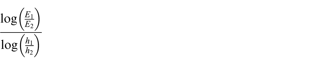
Here, we present some test problem to verify the developed method. To demonstrate the accuracy of this method, we use $L_{\infty }$ norm for computing errors. Also, the computational orders of the presented method (denoted by C-Order) is calculated using the following formula

$$\frac{\log \left(\frac{E_1}{E_2}\right)}{\log \left(\frac{h_1}{h_2}\right)}$$

where $E_i$ is the error value that corresponds to grid with mesh size $h_i$ .

Test problem 1

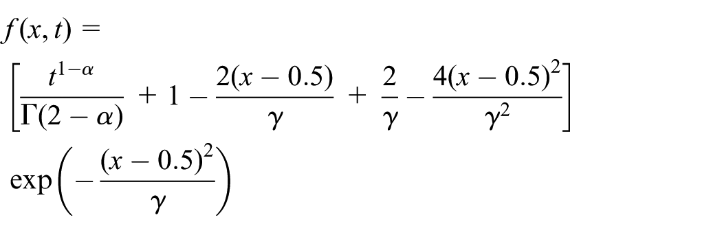
We consider the time fractional mobile/immobile equation with the form described in equation (1), where

$$f(x,t)=\left[\frac{t^{1-\alpha }}{\Gamma (2-\alpha )}+1-\frac{2(x-0.5)}{\gamma }+\frac{2}{\gamma }-\frac{4{(x-0.5)}^2}{{\gamma }^2}\right]\exp \left(-\frac{{(x-0.5)}^2}{\gamma }\right)$$

where exact solution is a Gaussian pulse with t height centered at $x=0.5$ , that is

$$u(x,t)=t\exp (-\frac{{(x-0.5)}^2}{\gamma })$$

boundary and initial conditions can be obtained from the exact solution.

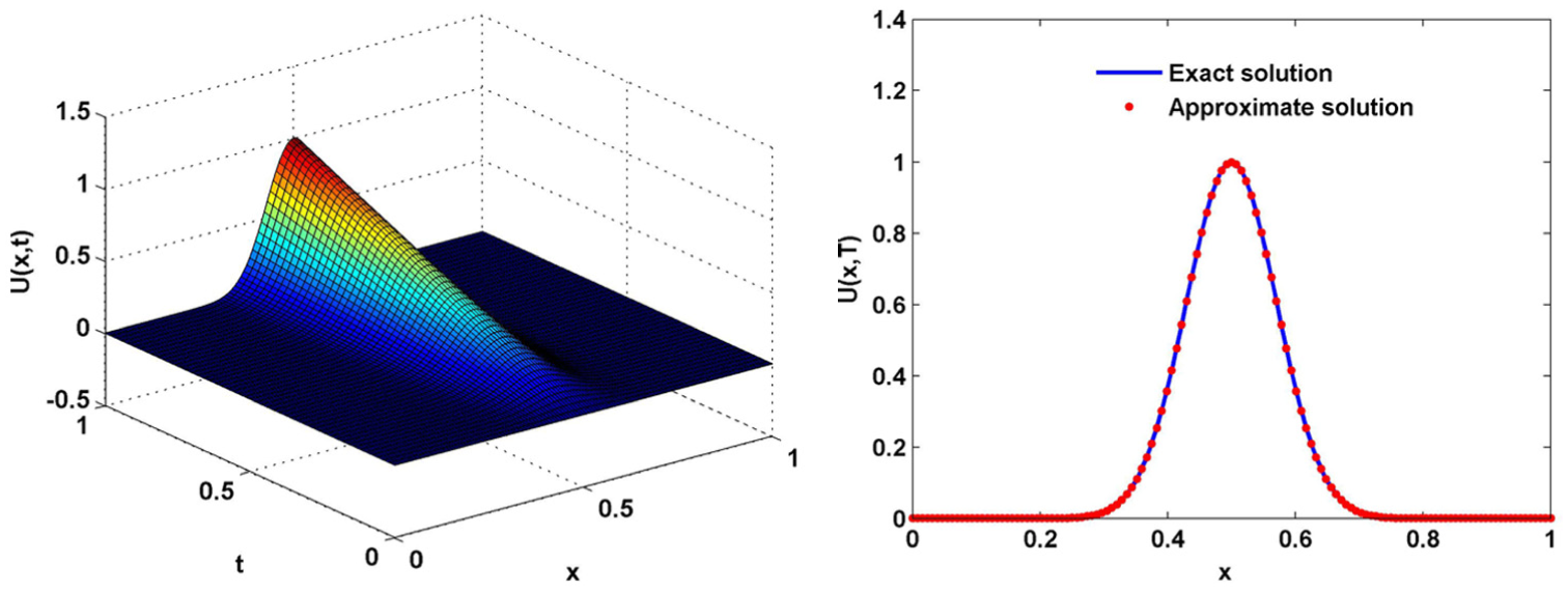
Table 1 demonstrates the $L_{\infty }$ error, computational order and total central processing unit (CPU) time (in second). The computational order of Table 1 is closed to the theoretical results. Figure 1 is based on $\alpha =0.35$ , $h=1/256$ , and $\tau =1/10$ . Also, the used parameter in Figure 2 is $\alpha =0.65$ , $\gamma =0.001$ , $h=1/128$ , and $\tau =1/50$ .

Table 1.

Evaluated computational orders and errors with $\tau =0.02$ and $\gamma =1/30$ , for Test problem 1.

h	$\alpha =0.25$		$\alpha =0.75$		CPU time (s)
	$L_{\infty }$	C-order	$L_{\infty }$	C-order
$1/4$	$7.1511\times {10}^{-1}$	−	$7.0721\times {10}^{-1}$	−	$00.3280$
$1/8$	$1.3344\times {10}^{-2}$	$5.7439$	$1.3344\times {10}^{-2}$	$5.7279$	$00.5000$
$1/16$	$7.0041\times {10}^{-4}$	$4.2518$	$7.0052\times {10}^{-4}$	$4.2516$	$00.8280$
$1/32$	$4.2169\times {10}^{-5}$	$4.0539$	$4.2177\times {10}^{-5}$	$4.0539$	$01.5310$
$1/64$	$2.6181\times {10}^{-6}$	$4.0096$	$2.6123\times {10}^{-6}$	$4.0131$	$02.7040$
$1/128$	$1.6394\times {10}^{-7}$	$3.9972$	$1.6398\times {10}^{-7}$	$3.9937$	$05.2030$
$1/256$	$1.0241\times {10}^{-8}$	$4.0480$	$1.0244\times {10}^{-8}$	$4.0007$	$10.2500$
$1/512$	$6.3905\times {10}^{-10}$	$4.0023$	$6.4120\times {10}^{-10}$	$3.9978$	$10.2500$

CPU: central processing unit.

Figure 1.

Approximated solutions and obtained errors for different values of $\gamma$ using presented method from (a) to (h) for Test problem 1.

Figure 2.

(Left) Surface plot of approximated solution; (right) exact and approximated solution with $\alpha =0.65$ , $\gamma =0.001$ , $\tau =1/50$ , and $h=1/128$ for Test problem 1.

Also, in Table 2, we can see error obtained with $h=\tau$ and different values of $\alpha$ for this problem.

Table 2.

Test problem 1 error values obtained for different parameters.

$h=\tau$	$\gamma =1/10$		$\gamma =1/100$
	$\alpha =0.4$	$\alpha =0.9$	$\alpha =0.4$	$\alpha =0.9$
$1/0$	$5.2339\times {10}^{-4}$	$5.2262\times {10}^{-4}$	$1.0742\times {10}^{-1}$	$1.0727\times {10}^{-1}$
$1/15$	$1.0297\times {10}^{-4}$	$1.0280\times {10}^{-4}$	$7.3552\times {10}^{-3}$	$7.3558\times {10}^{-3}$
$1/25$	$1.3323\times {10}^{-5}$	$1.3300\times {10}^{-5}$	$1.1490\times {10}^{-3}$	$1.1491\times {10}^{-3}$
$1/50$	$8.2954\times {10}^{-7}$	$8.2808\times {10}^{-7}$	$8.1048\times {10}^{-5}$	$8.1056\times {10}^{-5}$
$1/100$	$5.1797\times {10}^{-8}$	$5.1705\times {10}^{-8}$	$5.0049\times {10}^{-6}$	$8.0054\times {10}^{-6}$

Test problem 2

Again, we consider the time fractional mobile/immobile equation with the form described in equation (1) with source term

$$\begin{array}{l}f(x,t)=10x^2{(1-x)}^2\left(1+\frac{t^{1-\alpha }}{\Gamma (2-\alpha )}\right)\\ +10(t+1)\left(-2+14x-18x^2+4x^3\right)\end{array}$$

when boundary and initial conditions are of the following form

$$\begin{array}{c}u(0,t)=u(1,t)=0\hfill \\ \multicolumn{1}{c}{u(x,0)=10x^2{(1-x)}^2}\end{array}$$

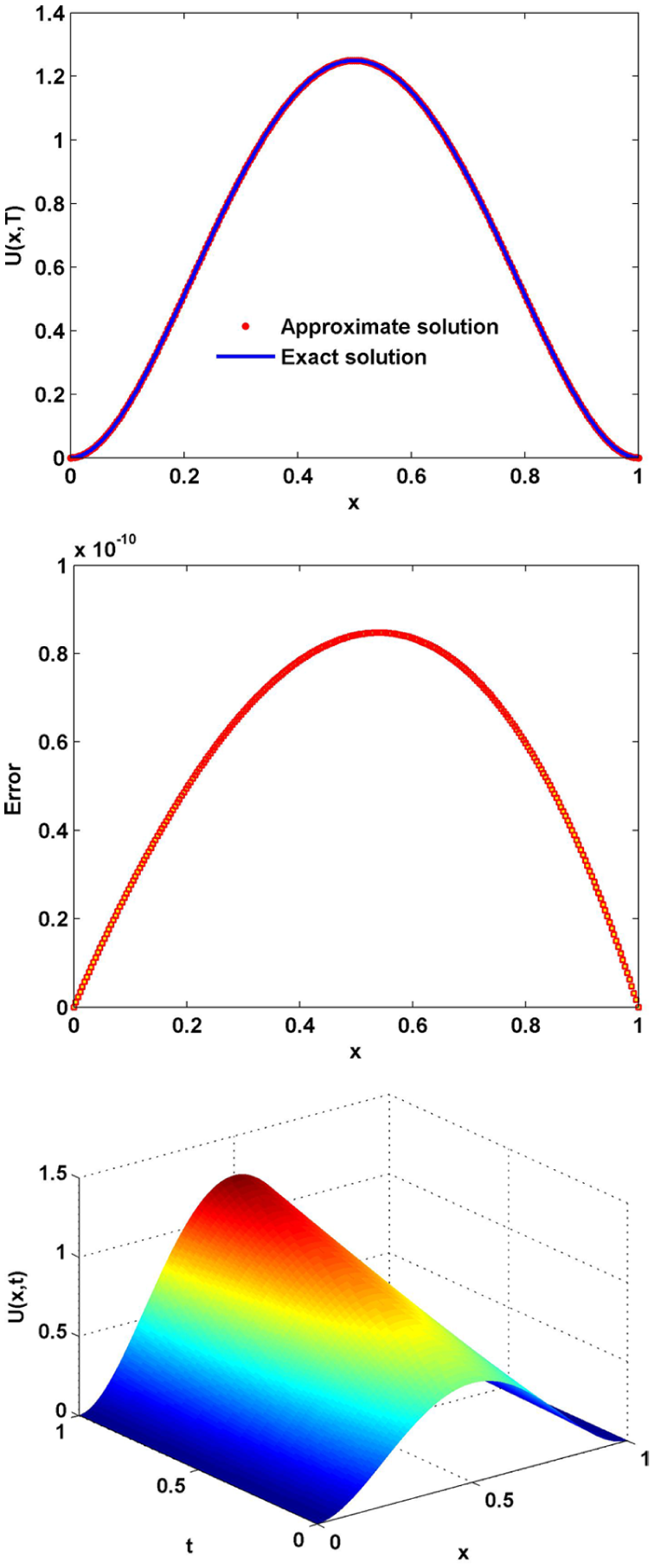
In this case the exact solution is as follows (Figure 3)

$$u(x,t)=10(1+t)x^2(1-x{)}^2$$

Figure 3.

Graphs of exact and approximate solution, absolute error, and surface plot of approximated solution with parameters $\alpha =0.45$ , $\tau =0.025$ , and $h=1/256$ , for Test problem 2.

In Table 3, we compare the errors obtained with the method of this article and method of Zhang et al. ¹² where $\alpha =1-0.5\exp (-x)$ . We see that the present method has good results in comparison with the method of Zhang et al. ¹² Computational order, $L_{\infty }$ error and CPU time (in seconds) are shown in Table 4. Also, Table 5 presents the error of numerical results for this problem with different values of parameters $\alpha$ and $\tau$ . Figure 3 demonstrates graphs of exact and approximate solution, absolute error, and surface plot of approximated solution with parameters $\alpha$ = 0.45, $\tau$ = 0.025, and h = 1/256, for Test problem 2.

Table 3.

Comparison of numerical solutions and errors obtained with $h=\tau =1/100$ for Test problem 1.

x	Exact solution	Method of Zhang et al. 12		Present method
		Numerical solution	$L_{\infty }$	Numerical solution	$L_{\infty }$
$0.1$	$0.162000$	$0.161843$	$1.5629\times {10}^{-4}$	$0.161999$	$1.1560\times {10}^{-9}$
$0.2$	$0.512000$	$0.510599$	$1.4006\times {10}^{-3}$	$0.511999$	$2.1029\times {10}^{-9}$
$0.3$	$0.882000$	$0.879024$	$2.9752\times {10}^{-3}$	$0.881999$	$2.8325\times {10}^{-9}$
$0.4$	$1.152000$	$1.147702$	$4.2977\times {10}^{-3}$	$1.151999$	$3.3312\times {10}^{-9}$
$0.5$	$1.250000$	$1.245027$	$4.9722\times {10}^{-3}$	$1.249999$	$3.5813\times {10}^{-9}$
$0.6$	$1.152000$	$1.147196$	$4.8034\times {10}^{-3}$	$1.151999$	$3.5579\times {10}^{-9}$
$0.7$	$0.882000$	$0.878184$	$3.8152\times {10}^{-3}$	$0.881999$	$3.2303\times {10}^{-9}$
$0.8$	$0.512000$	$0.509725$	$2.2746\times {10}^{-3}$	$0.511999$	$2.5610\times {10}^{-9}$
$0.9$	$0.162000$	$0.161279$	$7.2075\times {10}^{-4}$	$0.161999$	$1.5031\times {10}^{-9}$

Table 4.

Evaluated computational orders and error values with $\tau =1/50$ for Test problem 2.

h	$\alpha =0.1$		$\alpha =0.8$		CPU time (s)
	$L_{\infty }$	C-order	$L_{\infty }$	C-order
$1/4$	$1.3792\times {10}^{-3}$	−	$1.4064\times {10}^{-3}$	−	$00.0982$
$1/8$	$8.6206\times {10}^{-5}$	$3.9999$	$8.7903\times {10}^{-5}$	$3.9999$	$00.3910$
$1/16$	$5.4151\times {10}^{-6}$	$3.9937$	$5.5184\times {10}^{-6}$	$3.9936$	$00.7500$
$1/32$	$3.3877\times {10}^{-7}$	$3.9976$	$3.4545\times {10}^{-7}$	$3.9977$	$01.5620$
$1/64$	$2.1176\times {10}^{-8}$	$3.9998$	$2.1594\times {10}^{-8}$	$3.9998$	$02.9840$
$1/128$	$1.3236\times {10}^{-9}$	$3.9999$	$1.3495\times {10}^{-9}$	$4.0001$	$05.3750$
$1/256$	$8.2376\times {10}^{-11}$	$4.0061$	$8.1819\times {10}^{-11}$	$4.0438$	$10.7960$

CPU: central processing unit.

Table 5.

Error values obtained with different values of $\alpha$ and $\tau$ for Test problem 4.

$h=\tau$	$\alpha =0.25$	$\alpha =0.45$	$\alpha =0.65$	$\alpha =.85$
$1/10$	$3.5303\times {10}^{-5}$	$3.5414\times {10}^{-5}$	$3.5646\times {10}^{-5}$	$3.6012\times {10}^{-5}$
$1/15$	$7.0195\times {10}^{-6}$	$7.0435\times {10}^{-6}$	$7.0917\times {10}^{-6}$	$7.1674\times {10}^{-6}$
$1/25$	$9.0879\times {10}^{-7}$	$9.1207\times {10}^{-7}$	$9.1849\times {10}^{-7}$	$9.2857\times {10}^{-7}$
$1/50$	$5.8161\times {10}^{-8}$	$5.7111\times {10}^{-8}$	$5.7520\times {10}^{-8}$	$5.6898\times {10}^{-8}$

Conclusion

In this article, we built a compact difference scheme for the solution of time fractional mobile/immobile equation. We proved the unconditional stability property and convergence by Fourier analysis. It was shown that the numerical simulations obey the theoretical results. Examples are given and when the results obtained using this method with exact solutions are compared, this method shows applicability and efficiency.