Sage Journals: Discover world-class research

Abstract

Asymmetrical rail grinding in sharp-radius curves could reduce the side wear of railheads and enhance curve capacity of rail vehicles. The wheel/rail contact performance and curve capacity could be further improved by the optimization of the asymmetrical rail grinding target profile. In order to modify the target profile smoothly, the nonuniform rational B-spline curve with adjustable weight factors is used to establish a parameterized model of railhead curves in the asymmetrical grinding region. The indices of contact performance and curve capacity for different weight factors are obtained using experiment design and service performance simulation. Two Kriging surrogate models are proposed, in which the design variables are the adjustable weight factors, and the response parameters are the indices of contact performance and curve capacity, respectively. The multi-objective optimization model of the target profile is established, in which the objective functions are the two Kriging surrogate models of contact performance and curve capacity. The optimized weight factors are sought using a nondominated sorting genetic algorithm II, and the corresponding optimal target profile is obtained. The wheel/rail service performance simulation before and after optimization indicates that the contact performance and curve capacity are improved significantly.

Keywords

Asymmetrical rail grinding Kriging nonuniform rational B-spline sharp-radius curve target profile

Introduction

With the increase in speed and quantity of rail vehicles, rail side wear has become important in sharp-radius curves (for the passenger train operating at speed up to 250 km/h, the sharp curve means that the curvature radius is <4000 m), and rail corrosion has fallen into the category of rail damage.¹ It may improve the guidance ability by increasing rolling radius difference of wheelsets, reduce the wear between flange and inner side of rail, and prolong the rail service life three times by means of asymmetrical rail grinding in sharp-radius curves.^2,3 A reasonable target profile of asymmetrical rail grinding could guarantee the grinding quality and improve the wheel/rail relation in sharp-radius curves significantly. Therefore, some researchers have focused on the optimization of the target profile for asymmetrical rail grinding in sharp-radius curves. In order to improve the rail grinding quality in curves, and to decrease the cost of rail grinding, Sroba et al.⁴ designed several grinding target profiles with differential rail gauge corners to obtain the optimal grinding target profile in curves. For the purpose of obtaining a reasonable rolling radius difference and reducing contact stress, Jia and Si⁵ designed an optimal grinding target profile in sharp-radius curves based on practical rail grinding experience. Xiao and Liu³ took the corresponding railhead silhouettes in differential rail cants as the rail grinding target profiles and set the effective conicity, contact stress, and grinding amount as evaluation indices to obtain an optimal rail grinding target profile. For reducing the coefficient of derailment and improving the travel safety, H Doi⁶ grounded the region of a rail gauge corner in a curve and optimized the grinding target profile. Zhou et al.⁷ optimized the average wearing rail profile by the wheel/rail contact angle curve inverse method in curves, improving the wheel/rail contact status in curves. In order to form a conformal contact, Zhou et al.⁸ optimized the grinding target profile of 60N, which decreased the contact stress of the wheel/rail and reduced the grinding amount greatly.

Previous work designed optimal rail grinding target profiles in sharp-radius curves based on practical rail grinding experience and determined the corresponding grinding solution. Wheel/rail contact performance is drastically improved, and the guidance ability of wheelset for rail vehicles is enhanced. But the designed optimal asymmetrical rail grinding target profiles are all determined based on experience: the parameterized model of the rail grinding target profile is not constructed. This means that the asymmetrical rail grinding target profiles cannot be adjusted smoothly and precisely, which would cause the problem that the designed asymmetrical rail grinding target profiles are sub-optimal; the grinding quality could not be guaranteed either.

This work focuses on the construction of a parameterized model of the asymmetrical rail grinding target profile using the nonuniform rational B-spline (NURBS) curve, taking weight factors of the NURBS curve as the adjusted variables for the railhead curve of the parameterized model. It solved the problem of the target profile not being adjusted continuously and precisely. Taking the weight factors as the design variables, two Kriging surrogate (KS) models of contact stress between outer rail and outer wheel, and wheel-diameter difference, are constructed. A multi-objective optimization model of asymmetrical rail grinding target profiles is established, in which the objective functions are the two KS models, and the optimization objectives are the minimum contact stress and the maximum wheel-diameter difference. Then, the precise optimal asymmetrical rail grinding target profile is designed using a multi-objective global optimization method.

The principle of asymmetrical rail grinding

The wheel/rail guidance of rail vehicles plays an important role in the change of the movement direction. It includes two guidance methods that depend on creep force moment and flange/rail contact. But the flange will contact with the inner side of the outer rail when the rail vehicle guiding depends on the flange in a curve, which will increase rail wear significantly. Therefore, the optimal wheel/rail guidance method in a curve depends on the creep force moment. The force and moment of the wheelset guiding depend on the creep force moment as shown in Figure 1.

Figure 1.

Force and moment of the wheelset in the creep force moment guidance method passing through a curve.

The creep force moment M is calculated using equation (1)³

M = 2 ξ (\frac{λ y^{*} S}{r} - \frac{S^{2}}{R})

(1)

where ξ is the creep coefficient, λ is the effective conicity of the tread, y^* is the lateral offset of the wheelset center off the pure rolling line, S is the half-distance between the contact points of the wheelset, r is the nominal rolling radius, and R is the curvature radius. The assumption underlying the equation is the wheelset should have an appropriate lateral displacement.

λ and y^* are calculated in equations (2) and (3) accordingly

λ = \frac{| r_{o} - r_{i} |}{r} = \frac{Δ r}{2}

(2)

y^{*} = y - y_{0} = y - \frac{rs}{2 R λ}

(3)

where R is the radius of railway curve; r_i and r_o are the rolling radii of the inner and outer wheel, respectively; y is the lateral offset of the wheelset; y₀ is the lateral offset of the wheelsets in pure rolling; and Δr is the radius difference between inner and outer wheel, respectively, calculated in equation (4)

Δ r = | r_{o} - r_{i} | = 2 λ y

(4)

From equations (1)–(4), the effective conicity of the tread J and the lateral offset y^* will increase with Δr when the lateral offset y remains constant, and the creep force moment M will also increase. It is beneficial for the wheelset to pass through the curve using the creep force moment guidance method, which means that the wheel/rail correlation will be improved.

With decrease in the side wear, the asymmetrical rail grinding could also reduce the shelling defects in gauge corner. But this requires grinding the gauge corner of the outer rail, which will decrease the rolling radius of the outer wheel; the guidance ability of wheelset will also decline.⁹ Therefore, the gauge corner of the outer rail is not the key grinding region,³ and it will not be ground in this work. The key regions of asymmetrical rail grinding are shown in Figure 2.

Figure 2.

Asymmetrical rail grinding region in a sharp-radius curve.

The contact point of the outer rail in a curve moves from $c_{o}$ to $c'_{o}$ , and the rolling radius increases from $r_{o}$ to $r'_{o}$ after asymmetrical grinding. The contact point of the inner rail in a curve also moves from $c_{o}$ to $c'_{o}$ , and the rolling radius decreases from $r_{o}$ to $r'_{o}$ . Therefore, the radius difference between the outer rail and the inner rail $Δ r$ increases from $r_{o} - r_{i}$ to $r'_{o} - r'_{i}$ , which is beneficial for the train to pass through the curve via the creep force moment guidance method, meaning that the curve capacity of the rail vehicle will be improved.

Parameterization of the railhead curve of asymmetrical rail grinding

In order to analyze the corresponding contact stress σ_max and the rolling radius difference of the inner/outer wheel Δr in differential asymmetrical rail grinding target profiles, multi-groups of rail grinding target profiles with different railhead curves should be designed. As the asymmetrical rail grinding is aimed at a local region of a railhead curve, the parameterized model of the railhead curve must have the function to adjust the curve shape locally. An NURBS curve is a unified mathematical form that is used to describe standard analytical curves and free curves. It could also modify the local shape of a curve by moving reference points or adjusting weight factors.¹⁰ Therefore, it is widely used in the curve parameterization of engineering structures. The cubic NURBS curve will be able to meet the requirements of engineering applications in practical settings.¹¹ Therefore, the cubic NURBS curve is selected to establish the parameterized model of the railhead curve.

The NURBS curve

An NURBS curve of degree p¹⁰ could be defined as follows

C (u) = \frac{\sum_{i = 0}^{n} N_{i, p} (u) w_{i} P_{i}}{\sum_{i = 0}^{n} N_{i, p} (u) w_{i}}, a \leq u \leq b

(5)

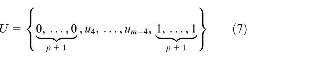
where {P_i} are the reference points, {w_i} are the weight factors, and {N_i,p(u)} are the B-spline basis functions of degree p that are defined in the aperiodic and nonuniform knot vector U (u₀, u₁,…, u_m). The {N_i,p(u)} are defined in equation (6)

\begin{matrix} N_{i, 0} = {\begin{matrix} 1, u_{i} \leq u \leq u_{i + 1} \\ 0, others \end{matrix} \\ N_{i, p} = \frac{u - u_{i}}{u_{i + p} - u_{i}} N_{i, p - 1} (u) + \frac{u_{i + p + 1} - u}{u_{i + p + 1} - u_{i + 1}} N_{i + 1, p - 1} (u) \end{matrix}

(6)

where U is calculated in equation (3)

U = {\underset{p + 1}{\underset{︸}{0, \dots, 0}}, u_{4}, \dots, u_{m - 4}, \underset{p + 1}{\underset{︸}{1, \dots, 1}}}

(7)

Parameterization of the railhead curve based on cubic NURBS curve

An NURBS curve is defined by reference points {P_i}, weight factors {w_i}, and knot vector U, and the curve shape will change with the modification of any {P_i}, {w_i}, or U. In order to reduce computational effort and ensure the continuity and smoothness of the adjustment of the target profile, in this study, we adjust the local region of the railhead curve by modifying the weight factors {w_i}, after which the parameterized model of the railhead curve based on adjustable weight factors is constructed.

The railhead curve of the 60N used in Chinese trunk routes is taken as the object to construct the NURBS parameterized curve of the asymmetrical rail grinding target profile. The curve segment that could contact with the tread, as shown in Figure 3(a), is selected to be parameterized. Polar coordinates are used, using the center of the railhead curve as the origin. Then, 23 points are selected uniformly in the parameterized railhead curve as the data points, considering the adjustment accuracy and the number of the adjustment variables. The reference points {P₁,…, P₂₅}, shown in Figure 3(b), are reconstructed using the NURBS interpolation method.¹² The knot vector U is calculated using the chord length parameterization method,¹⁰ and all of the weight factors {w_i} in each reference point are preset to 1. Then, the parameterized model of the asymmetrical rail grinding target profile is established, in which the segment of the railhead curve could be adjusted locally by modifying the weight factors.

Figure 3.

Parameterized model of the asymmetrical rail grinding target profile based on cubic NURBS curve: (a) the railhead silhouette of 60N and (b) the parametric railhead curve.

The adjustment of the railhead curve based on adjustable weight factors

The region of the asymmetrical rail grinding is the outside railhead of the outer rail and the inside railhead of the inner rail, based on Figure 2. It is also the region controlled by the weight factors w₁₆, w₁₇, and w₁₈ contrasting with the parameterized railhead curve shown in Figure 3(b). Different asymmetrical rail grinding profiles, with differential railhead curves, will be obtained by modifying the adjustable weight factors w₁₆, w₁₇, and w₁₈. The contrast of different target profiles with differential railhead curves in the grinding region is shown in Figure 4, when w₁₆, w₁₇, and w₁₈ take different values.

Figure 4.

Contrast of railhead curves in the grinding region with differential weight factors.

Simulation of service performance for different target profiles

Evaluation indices of service performance for the target profile

Reducing rail side wear and improving the curve capacity of the wheelset are two important targets of asymmetrical rail grinding. Reducing the contact stress of the wheel/rail and increasing the rolling radius difference of the inner/outer wheel could achieve the two targets.¹³ Therefore, the contact stress of the outer guidance wheelset and the rolling radius difference of the inner/outer wheels are taken as the two optimization indices.

Contact stress of wheel/rail

Increasing effective conicity usually reduces side wear, although it often increases contact stress.³ Therefore, the wheel/rail contact stress should be reduced. The maximum contact stress σ_max is calculated in equation (8) based on the Hertz contact stress¹⁴

σ_{max} = \frac{3 P}{2 A}

(8)

where P is the maximum wheel/rail normal force in the contact zone and A is the area of the contact zone.

Rolling radius difference of the inner/outer wheel

As the creep force moment M increases with the rolling radius difference of the inner/outer wheel Δr, the vehicle will pass through the curve following the creep force moment guidance method. Therefore, Δr becomes an important index to evaluate the result of the asymmetrical rail grinding. In order to improve the curve capacity of the wheelset, Δr should be increased as much as possible. For the purpose of analyzing the impact of different rail grinding target profiles on Δr, the wheel/rail contact point trace line method,¹⁵ using spline functions to fit the rail and wheel tread, is used to obtain the y–Δr curve.

Simulation of service performance for different target profiles

Simulation model

Different asymmetrical rail grinding target profiles with differential railhead curves are obtained, while the differential adjustable weight factors w₁₆, w₁₇, and w₁₈ are taken to construct the NURBS curve. In order to determine the optimal target profile, the wheel/rail contact performance and curve capacity of differential asymmetrical rail grinding target profiles should be analyzed in differential target profiles. This analysis means that the contact stress σ of the outer wheel/rail and the rolling radius difference Δr of the inner/outer wheel need to be calculated for differential target profiles. A rail section with a rightward curve using the 60N rail is set in SIMPACK. The radius of the curve is 4000 m, the rail cant is 1:40, the track gauge is 1435 mm, and the super elevation of outer rail is 120 mm. The running vehicles are the CRH2 electrical multiple units, the tread of the wheelset is LMa (the concrete tread shape is shown in Figure 5), the wheel back distance is 1493 mm, the radius of the wheel is 430 mm, and the travel speed is 80 km/h. The simulation model of wheel/rail contact performance and curve capacity constructed in SIMPACK is shown in Figure 5, and the response quantities are taken when the train passes through the transition curve.

Figure 5.

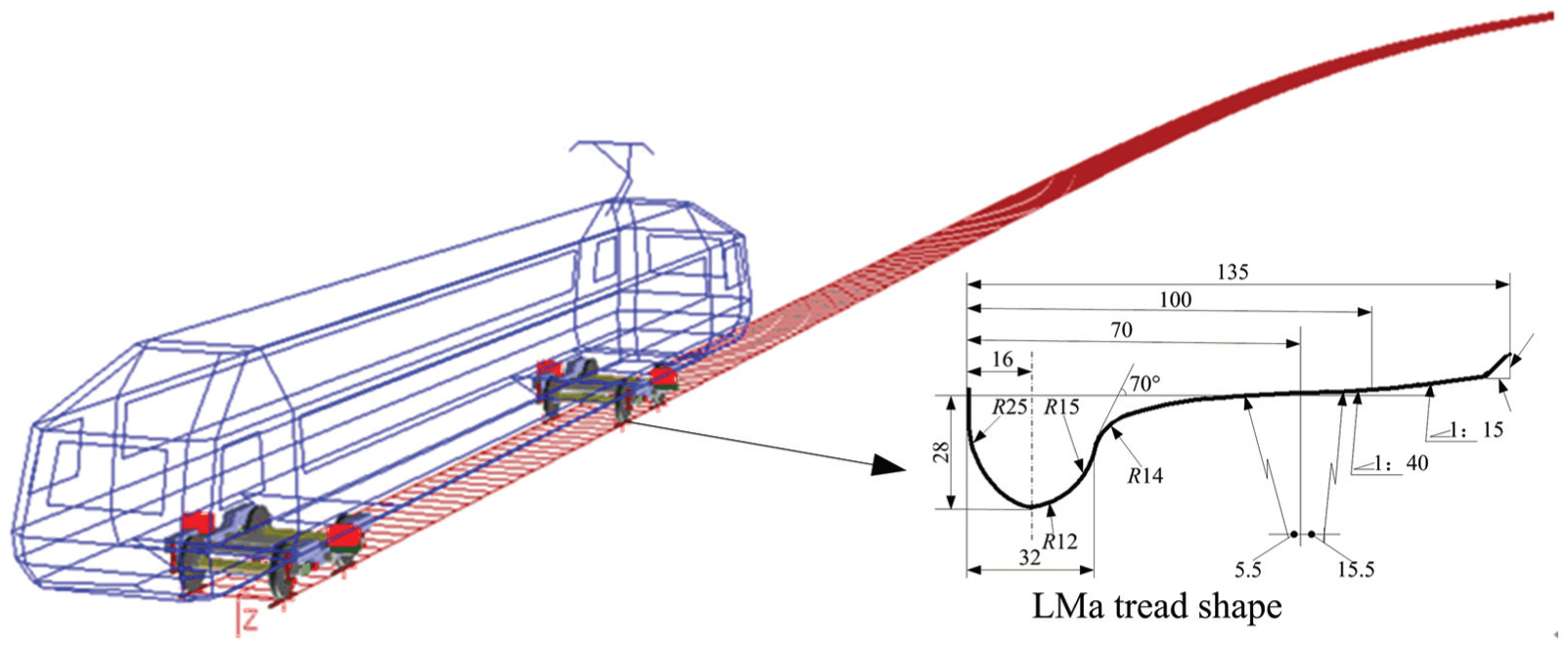
Model of wheel/rail contact performance and curve passage capacity.

Simulation process

As the value of the contact stress σ between the guiding wheel and outer rail is a maximum when the vehicle travels through a curve, the contact stress σ is selected as the index to evaluate the contact performance of the target profile. Meanwhile, the rolling radius difference Δr of the guiding wheelset is selected as the index to evaluate curve capacity. Several combinations of the adjustable weight factors w₁₆, w₁₇, and w₁₈ are obtained using the Latin hyper cubic sampling method, and the corresponding railhead curves are constructed using the parameterized model of the target profile. Then, the corresponding data files are imported to the analysis model to obtain the contact stress σ and the rolling radius difference Δr. The contact point with maximum contact stress and minimum rolling radius difference is selected as the data point, when multi-point contact condition appears. The specific analysis process is shown in Figure 6.

Figure 6.

Simulation process of the wheel/rail contact performance and curve passage performance.

KS models of wheel/rail performance and curve capacity

In order to construct the multi-objective optimization model of the asymmetrical rail grinding target profile, the objective functions need to be established to calculate the evaluation indices of many target profiles. Huge computational and low optimization efficiency will appear if the simulation method, as shown in Figure 6, is taken to calculate the evaluation indices of the repeated target profiles. A KS model is a kind of interpolation method with a smoothing effect and minimum variance estimation, considering spatial correlation of variables sufficiently.¹⁶ But additional time will be spent to construct a KS model, which would increase the optimization time, especially when the sampling points are huge. As it can forecast the dynamic transformation trend of variables based on the spatial correlation analysis of sample data, a KS model is used to fit the nonlinear characteristics of the wheel/rail contact stress and the curve capacity in this study.

Construction of KS models

Basic form of a KS model

A typical KS model is composed of two parts, a polynomial and a random distribution,¹⁶ as in equation (9)

y (X) = F (\hat{β}, X) + Z (X)

(9)

where X is the surrogate model variable space and $F (\hat{β}, X)$ is the regression model determined by known functions X that are calculated in equation (10)

\begin{matrix} F (\hat{β}, x) = {\hat{β}}_{1} f_{1} (x) + {\hat{β}}_{2} f_{2} (x) + \dots + {\hat{β}}_{n} f_{n} (x) \\ = \hat{β} {[f_{1} (x) f_{2} (x) + \dots + f_{n} (x)]}^{T} \\ = \hat{β} f^{T} (x) \end{matrix}

(10)

where $\hat{β}$ is the regression coefficient of variables, f(x) is the base function, and n is the number of training samples.

Z(X) are the errors of random distribution, and their mean value is 0. Additionally, the variance is $σ_{Z}^{2}$ , and the covariance is given by

Cov [Z (x_{i}), Z (x_{j})] = σ^{2} R [R (x_{i}, x_{j})]

(11)

where x_i and x_j are any two points of the training sample and $[R (x_{i}, x_{j})]$ is the correlation function, which is used to describe the relationship between x_i and x_j. As the Gaussian correlation function is usually used in engineering applications, the correlation function could be written as

R (x_{i}, x_{j}) = \exp (- {\sum_{k = 1}^{h} θ_{k} | x_{k}^{i} - x_{k}^{j} |}^{2})

(12)

where h is the number of design variables and $x_{k}^{i}$ and $x_{k}^{j}$ are the corresponding kth components of x_i and x_j in the training sample.

The response value $\hat{y} (x)$ and an estimated value of variance $\hat{σ}$ at any point x can be calculated using equations (13) and (14)

\hat{y} (x) = \hat{β} + r {(x)}^{T} R^{- 1} (y - f \hat{β})

(13)

{\hat{σ}}^{2} = \frac{1}{n} {(y - f \hat{β})}^{T} R^{- 1} (y - f \hat{β})

(14)

where $r^{T}$ is a relevance vector of length n, f is a unit column vector of length n, and $\hat{β} = (f^{T} R^{- 1} y)^{- 1} f^{T} R^{- 1} y$ .

θ_k is the value of maximum likelihood estimation (MLE), which is calculated from equation (15)

MLE = max_{θ_{k} > 0} {- \frac{1}{2} [h \ln ({\hat{σ}}^{2}) + \ln | R |]}

(15)

where the variance $\hat{σ}$ is calculated by equation (14). The relevance vector r^T between an unknown point and known sample data points could be calculated after the correlation parameter θ_k is obtained. Then, the response value of the wheel/rail contact stress σ and rolling radius difference Δr are calculated using equation (9).

Construction of KS models

Taking the adjustable weight factors w₁₆, w₁₇, and w₁₈ as the design variables of the KS model based on the parameterized model of the asymmetrical rail grinding target profile shown in Figure 3. The KS models of wheel/rail contact performance and curve capacity are established in the construction, as shown in Figure 7.

Figure 7.

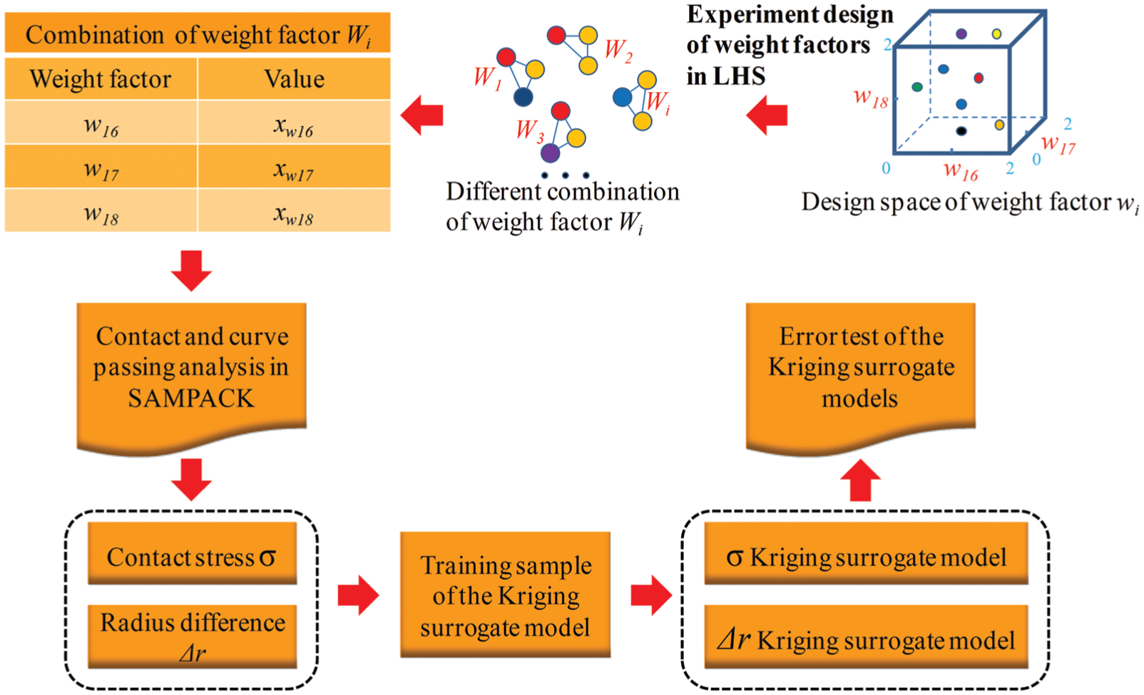
Construction of KS models.

Several groups points of weight factors are sampled in the experimental design method after the value ranges of the design variables as w₁₆, w₁₇, and w₁₈ are determined. The indices of wheel/rail contact performance σ and curve capacity Δr under different combinations of adjustable weight factors are simulated in the analysis process, as shown in Figure 6. The corresponding indices are taken as the training samples to construct KS models of wheel/rail contact performance and curve capacity. And an error test method is taken to guarantee the fitting accuracy of the KS model.

Experiment design

Multiple groups of sample points of adjustable weight factors need to be obtained during the modeling of KS models of wheel/rail contact performance and curve capacity. The Latin hyper cubic experiment method is used to obtain sample points of adjustable weight factors, as it could sample uniformly, thus avoiding the data missing problem.¹⁷ The value ranges of the experiment design are shown in Table 1.

Table 1.

Value ranges of adjustable weight factors.

No.	Adjustable weight factors	Current value	Upper limit
1	w ₁₆	1	2
2	w ₁₇	1	2
3	w ₁₈	1	2

The number of training samples is usually three times the quadratic polynomial coefficient k in the modeling of a KS model, and the corresponding coefficient k = (n + 1)(n + 2)/2, n is the number of variables.¹⁸ As the number of design variables in this study is 3, so the number of training samples of the two KS models is 30.

A total of 30 groups of adjustable weight factors are obtained using the Latin hyper cubic experiment design method, and the corresponding wheel/rail contact stress σ and rolling radius difference Δr are simulated in the wheel/rail contact performance and curve capacity analysis process as shown in Figure 6. The simulation results are shown in Table 2.

Table 2.

Training samples of KS models.

No.	w ₁₆	w ₁₇	w ₁₈	Evaluation indices of target profiles
				σ	Δr
1	1.95249	0.541903	0.318814	1921.74	8.813
2	1.308123	0.232827	0.142763	1980.65	8.947
3	1.183405	1.680745	1.809266	2097.39	8.251
4	0.716476	0.968465	1.781071	2175.46	8.140
5	0.415517	1.544747	0.42564	3871.93	8.052
6	0.930009	1.445168	1.881367	2161.97	7.214
7	0.354314	0.40159	1.60301	1917.42	8.071
8	0.491981	0.314786	1.472026	2000.49	7.718
9	1.683554	1.061811	1.974346	2227.35	8.037
10	1.601516	1.949918	0.055824	3437.16	7.992
…	…	…	…	…	…
29	0.288095	0.754156	1.122051	2277.86	8.237
30	1.536933	1.828776	0.849437	2018.11	8.593

KS models of wheel/rail contact performance and curve capacity

The correlation matrix R and unit column vector f are calculated based on the training sample of the KS models, as shown in Table 2. The correlation coefficients of the two KS models ${\hat{β}}_{σ}$ and ${\hat{β}}_{Δ r}$ are calculated as follows

\begin{matrix} {\hat{β}}_{σ} = {({f^{T}}_{σ} {R^{- 1}}_{σ} y_{σ})}^{- 1} {f^{T}}_{σ} {R^{- 1}}_{σ} y_{σ} = 0.395 \\ {\hat{β}}_{Δ r} = {({f^{T}}_{Δ r} {R^{- 1}}_{Δ r} y_{Δ r})}^{- 1} {f^{T}}_{Δ r} {R^{- 1}}_{Δ r} y_{Δ r} = 0.005 \end{matrix}

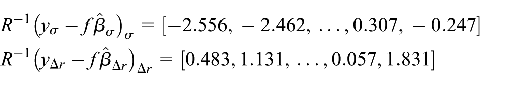
Then, $R^{- 1} (y - f \hat{β})$ is calculated using R, y, f, and $\hat{β}$

\begin{matrix} R^{- 1} {(y_{σ} - f {\hat{β}}_{σ})}_{σ} = [- 2.556, - 2.462, \dots, 0.307, - 0.247] \\ R^{- 1} {(y_{Δ r} - f {\hat{β}}_{Δ r})}_{Δ r} = [0.483, 1.131, \dots, 0.057, 1.831] \end{matrix}

The estimated value of unbiased variance ${\hat{σ}}^{2}$ of KS models is calculated using equation (14). Then, the correlation parameters of contact stress and rolling radius difference θ_kσ and θ_k_Δr are calculated using an MLE, as shown in equation (15). The concrete values of the correlation parameters are as follows

\begin{matrix} {θ_{k}}_{σ} & = [0.336 0.462 1.065] \\ {θ_{k}}_{Δ r} & = [2.000 2.000 1.999] \end{matrix}

The relevance vectors r^T are calculated after the correlation parameters θ_k are determined, and the response value of any unknown design point could be calculated. Then, the KS models of contact stress σ and rolling radius difference Δr are constructed as per Figure 8. The modeling time is 2.3 s, and the memory consumption is 216.3 M.

Figure 8.

KS models of wheel/rail contact performance and curve passage capacity: (a) KS model of σ and (b) KS model of Δr.

Error test

To guarantee the fitting accuracy of the constructed KS models of wheel/rail contact stress σ and rolling radius difference Δr, the root mean square error (RMSE)¹⁹ is used to estimate the fitting accuracy of the two KS models.

From equation (13), the mean square error (MSE) of any response value of the KS model is

MSE = E [(\hat{y} (x) - y {(x)}^{2})] = {\hat{σ}}^{2} (1 + μ^{T} {(f^{T} R^{- 1} f)}^{- 1} μ - r^{T} R^{- 1} r)

(16)

RMSE = \sqrt{MSE}

(17)

where µ = f^TR⁻¹r − fθ_k. To guarantee the accuracy of the KS model, the RMSE must be a minimum and >0. In the error testing, 10 groups of adjustable weight factors in Table 2 are selected randomly to plug into the KS models to calculate the fitting values of σ and Δr. Then, the fitting values of σ and Δr are compared to the corresponding values simulated by SIMPACK in Table 2. The RMSE values of the two KS models are 0.03119 and 0.04816, respectively.

Multi-objective optimization of the target profile

Multi-objective optimization model

To decrease side wear and improve the curve capacity of the rail vehicle, the contact stress value σ should be reduced and the rolling radius difference Δr should be increased as much as possible. Therefore, the multi-objective optimization model of the target profile is established, in which the optimization objectives are a smaller contact stress σ and a greater rolling radius difference Δr, the design variables are the adjustable weight factors W{w₁₆, w₁₇, w₁₈}, and the objective functions are the established two KS models of contact stress performance and curve capacity. The specific form of the multi-objective optimization model of the target profile is

\begin{matrix} find : w_{16}, w_{17}, w_{18} \\ min : σ (W) = f_{σ} {(W)}^{T} {\hat{β}}_{σ} + r_{σ}^{T} (W) R_{σ}^{- 1} (y_{σ} - F_{σ} {\hat{β}}_{σ}) \\ \max : Δ r (W) = f_{Δ r} {(W)}^{T} {\hat{β}}_{Δ r} + r_{Δ r}^{T} (W) R_{Δ r}^{- 1} (y_{Δ r} - F_{Δ r} {\hat{β}}_{Δ r}) \\ s . t . \\ 0 \leq w_{16} \leq 2 \\ 0 \leq w_{17} \leq 2 \\ 0 \leq w_{18} \leq 2 \\ V_{cr} \leq 300 km / h \end{matrix}

(18)

where $σ (W) = f_{σ} (W)^{T} {\hat{β}}_{σ} + r_{σ}^{T} (W) R_{σ}^{- 1} (y_{σ} - F_{σ} {\hat{β}}_{σ})$ is the KS model of wheel/rail contact performance, and $Δ r (W) = f_{Δ r} (W)^{T} {\hat{β}}_{Δ r} + r_{Δ r}^{T} (W) R_{Δ r}^{- 1} (y_{Δ r} - F_{Δ r} {\hat{β}}_{Δ r})$ is the KS model of curve capacity. w₁₆, w₁₇, and w₁₈ are the adjustable weight factors. V_cr is the critical speed.

Optimization of the adjustable weight factors based on nondominated sorting genetic algorithm II

The nondominated sorting genetic algorithm II (NSGA-II) has a superior searching performance, and its computation efficiency of the optimal solution of Pareto is improved so significantly that it selects the individuals close to the Pareto front as the elite individuals in the process of the optimizing.²⁰ Therefore, NSGA-II is selected as the multi-objective optimization algorithm to search for the optimum weight factors in equation (18). The initial pop size is 12, maximum generation is 200, and the crossover probability is 0.9. The whole 2400 interpolations of the optimization are shown in Figure 9.

Figure 9.

Interpolation process of adjustable weight factors using NSGA-II.

The optimizing target of the NSGA-II is to obtain the suitable adjustable weight factors that makes the contact stress value σ sufficiently small and rolling radius difference Δr sufficiently large. That is to say, the Pareto noninferior solution of the σ and Δr need to be searched. A relatively obvious Pareto front has been formed after 2400 interpolations from the interpolation process of adjustable weight factors, as shown in Figure 9. The Pareto solution of the σ and Δr fluctuates significantly in the first 450 interpolations and then converges to form a relatively stable Pareto solution. The concrete values of the contact stress σ and rolling radius difference Δr remain at 1500 and 9.0, respectively. Therefore, a stable Pareto noninferior solution of optimal adjustable weight factors, as shown in Figure 10, is found after 2400 iterations. And the optimization time is 4.7 s, and the memory consumption is 591.3 M. The optimal Pareto solution is shown in Table 3.

Figure 10.

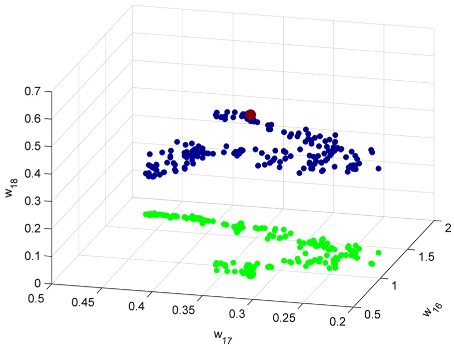
Pareto noninferior solution of the adjustable weight factors.

Table 3.

Initial values and optimal results of the adjustable weight factors.

Adjustable weight factors	w ₁₆	w ₁₇	w ₁₈
Initial value	1	1	1
Optimal results	0.910	0.324	0.580

Service performance of wheel/rail: contrast between original and optimal versions

The optimal weight factors of w₁₆, w₁₇, and w₁₈ are plugged into the parameterized railhead curve model of the asymmetrical rail grinding target profile based on an NURBS curve. Then, the optimal target profile is obtained, as shown in Figure 11.

Figure 11.

The optimal target profile of asymmetrical rail grinding.

The wheel/rail contact performance and curve capacity in sharp-radius curves are simulated using the process shown in Figure 6, in which the rail profile is the optimal target profile, as shown in Figure 11. The time-domain graph of contact stress and rolling radius difference is shown in Figure 12(a) and (b).

Figure 12.

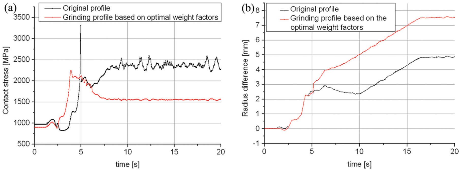
Contrast of wheel/rail contact performance and curve passage capacity between original and optimal versions: (a) time-domain graph of contact stress and (b) time-domain graph of rolling radius difference.

From the analysis of Figure 12(a), the contact stress value in the optimal target profile is almost equivalent with the original profile during the period 2.5–4.5 s. However, it decreased rapidly to remain around 1500 MPa, which is smaller than the corresponding value of 2250 MPa in the original target profile. This decrease means that the wheel/rail contact performance has been improved after optimization. From the analysis of Figure 12(b), the rolling radius difference in the optimal target profile is consistent with that of the original profile during the first 5 s. However, it then rapidly increased, which indicates that the curve capacity has been improved after optimization. Therefore, the effectiveness of the optimization method in this study is verified.

Conclusion

This article constructed the parameterized model of the asymmetrical rail grinding target profile in sharp-radius curves based on an NURBS curve. The indices of wheel/rail contact performance and curve capacity in differential asymmetrical rail grinding profiles are also simulated using the analysis model constructed in SIMPACK. The optimization model of the target profile based on the two established KS models of wheel/rail contact performance and curve capacity is constructed and then the optimum target profile is obtained by the optimization of the adjustable weight factors. Our principal conclusions are as follows:

The parameterized model of the asymmetrical rail grinding target profile in sharp-radius curves is constructed based on an NURBS curve. The weight factors of the NURBS curve are taken as the design variables, to adjust the railhead curve in the region of the asymmetrical rail grinding, and then the railhead curve could be adjusted continuously and smoothly.

The indices of wheel/rail contact performance and curve capacity in differential combinations of the adjustable weight factors are simulated using the model in SIMPACK. On this basis, two KS models of wheel/rail contact performance and curve capacity are constructed, which provide a high-fitting surrogate analysis model for the optimization of the target profile.

The multi-objective optimization model of the symmetrical rail grinding target profile is proposed, in which the objective functions are the two KS models of wheel/rail contact performance and curve capacity. The NSGA-II is employed in order to optimize the adjustable weight factors to obtain the optimum Pareto solution of the weight factors. Then, the optimum target profile of the asymmetrical rail grinding is obtained by plugging the optimum adjustable weight factors into the parameterized railhead curve model. The optimal results indicate that the wheel/rail contact stress value of the guidance wheel decreased significantly, and the rolling radius difference also increased, which demonstrates the viability of this method.

It must be admitted that the proposed approach is only validated by simulation, which cannot validate the effectiveness of the approach. And the actual physical experiment, combining with the control system of the rail grinding vehicle, should be carried out.

Footnotes

Academic Editor: Francesco Massi

Declaration of conflicting interests

The author(s) declared no potential conflicts of interest with respect to the research, authorship, and/or publication of this article.

Funding

The author(s) disclosed receipt of the following financial support for the research, authorship, and/or publication of this article: This research was undertaken at the CAD/CAM institute, Central South University, China. This work was supported by the Natural Science Foundation of Hunan Province (grant no. 2015JJ2168), the scientific research projects of Shanxi Province Education Department in China (grant no. 16JK2242), and the project (grant no. 51405516) of the National Natural Science Foundation in China.

References

Cuervo

Santa

Toro

Correlations between wear mechanisms and rail grinding operations in a commercial railroad. Tribol Int 2015; 82: 265–273.

Craven

Bewes

Fenech

. Responding to the Environmental Noise Directive by demonstrating the benefits of rail grinding on the Great Britain’s* railway network. Proc IMechE, Part F: J Rail and Rapid Transit 2013; 227: 668–676.

Xiao

Liu

Design method of rail asymmetric silhouette. J Southwest Jiaotong Univ 2010; 45: 361–365.

Sroba

Magel

Prahl

RT and S: improved profiles need special grinding. Railw Track Struct 2004; 100: 26–28.

Jia

Target profile of rail grinding for small radius curve of Shuohuang railway. China Railw Sci 2014; 35: 15–21.

Doi

. A study on relationship between rail grinding and flange climbing of railway vehicle at low speed in curve. Trans Jpn Soc Mech Eng C 2011; 77: 3325–3336.

Zhou

Liu

Peng

Optimization of rail profile in curved section of railway passenger dedicated line. Railw Stand Des 2014; 58: 20–23.

Zhou

Yinhua

Changhai

. Profile design and test study of 60N rail. China Railw Sci 2014; 35: 128–135.

Lian

Sun

Wang

The rail curve rail abrasion and its mitigation measures. Beijing, China: China Railway Publishing House, 2001, p.126.

10.

Piegl

Tiller

The NURBS book. Beijing, China: Tsinghua University Press, 2010, p.86.

11.

Espath

LFR

Braun

Awruch

. NURBS-based three-dimensional analysis of geometrically nonlinear elastic structures. Eur J Mech A: Solid 2014; 47: 373–390.

12.

Chen

Interpolation and application for cubic NURBS curves. Mech Sci Techonl 2001; 20: 692–693.

13.

Adachi

Matsumoto

Improvement of curving performance by expansion of gauge widening and additional measures. Proc IMechE, Part F: J Rail and Rapid Transit 2012; 226: 203–215.

14.

Ashofteh

RS.

Calculating the contact stress resulting from lateral movement of the wheel on rail by applying hertz theory. Int J Railw 2013; 6: 148–154.

15.

Wang

The track of wheel contact points and the calculation of wheel/rail geometric contact parameters. J Southwest Jiaotong Univ 1984; 19: 89–99.

16.

Lee

Kim

Kriging-based approximate optimization of high-speed train nose shape for reducing micropressure wave. Proc IMechE, Part F: J Rail and Rapid Transit 2007; 221: 263–270.

17.

Roshanian

Ebrahimi

Latin hypercube sampling applied to reliability-based multidisciplinary design optimization of a launch vehicle. Aerosp Sci Technol 2013; 28: 297–304.

18.

Yang

Zeng

Wen-Sheng

. Optimization of the suspension parameters of a rail vehicle based on a virtual prototype Kriging surrogate model. Proc IMechE, Part F: J Rail and Rapid Transit. Epub ahead of print 19 January 2016. DOI: 10.1177/0954409715617213.

19.

Wei

Yue

Huan

. CF-Kriging surrogate model based on the combination forecasting method. Proc IMechE, Part C: J Mechanical Engineering Science. Epub ahead of print 5 October 2015. DOI: 10.1177/0954406215610149.

20.

Khalkhali

Best compromising crashworthiness design of automotive S-rail using TOPSIS and modified NSGAII. J Cent South Univ 2015; 22: 121–133.

Optimization of the target profile for asymmetrical rail grinding in sharp-radius curves for high-speed railways

Abstract

Keywords

Introduction

The principle of asymmetrical rail grinding

Parameterization of the railhead curve of asymmetrical rail grinding

The NURBS curve

Parameterization of the railhead curve based on cubic NURBS curve

The adjustment of the railhead curve based on adjustable weight factors

Simulation of service performance for different target profiles

Evaluation indices of service performance for the target profile

Contact stress of wheel/rail

Rolling radius difference of the inner/outer wheel

Simulation of service performance for different target profiles

Simulation model

Simulation process

KS models of wheel/rail performance and curve capacity

Construction of KS models

Basic form of a KS model

Construction of KS models

Experiment design

KS models of wheel/rail contact performance and curve capacity

Error test

Multi-objective optimization of the target profile

Multi-objective optimization model

Optimization of the adjustable weight factors based on nondominated sorting genetic algorithm II

Service performance of wheel/rail: contrast between original and optimal versions

Conclusion

Footnotes

Declaration of conflicting interests

Funding

References