Sage Journals: Discover world-class research

Abstract

In this article, we study the economic lot and delivery scheduling problem for a four-stage supply chain that includes suppliers, fabricators, assemblers, and retailers. All of the parameters such as demand rate are deterministic and production setup times are sequence-dependent. The common cycle time and integer multipliers policies are adapted as replenishment policies for synchronization throughout the supply chain. A new mixed integer nonlinear programming model is developed for both policies, the objective of which is the minimization of inventory, transportation, and production setup costs. We propose a new hybrid algorithm including a modified imperialist competitive algorithm which is purposed to the assimilation policy of imperialist competitive algorithm and teaching learning–based optimization which is added to improve local search. A hybrid modified imperialist competitive algorithm and teaching learning–based optimization is applied to find a near-optimum solution of mixed integer nonlinear programming in large-sized problems. The results denoted that our proposed algorithm can solve different size of problem in reasonable time. This procedure showed its efficiency in medium- and large-sized problems as compared to imperialist competitive algorithm, modified imperialist competitive algorithm, and other methods reported in the literature.

Keywords

Supply chain management mixed integer nonlinear programming scheduling coordination imperialist competitive algorithm teaching learning–based optimization

Introduction

The coordination of the chain members is one of the important objectives of supply chain since members of each stage have different and even opposite profit. Synchronization can increase coordination among the chain members. The synchronization causes balance between decision making for internal production scheduling and the external delivery in the chain. One of the prevalent problems in the literature that examines these two cases simultaneously is economic lot and delivery scheduling problem (ELDSP).

Hahm and Yano¹ studied a supply chain consisting of one supplier and one assembler and could determine the interval between production and delivery for a single item. They developed this problem for multiple items and presented a heuristic algorithm for determining the common cycle time.² Khouja³ studied this problem with the assumption of rework cost for achieving the required quality and also variable production rate. Jensen and Khouja⁴ presented a heuristic algorithm for achieving the optimal solution in polynomial time. Their work is developed by Clausen and Ju.⁵ They proposed a heuristic algorithm to find the optimal solution of large-scale problem at a shorter time.

Torabi et al.⁶ studied a two-stage supply chain including one supplier and one assembler and multiple items with the common cycle time. They proposed a hybrid genetic algorithm (GA) for the solution of ELDSP. Nikandish et al.⁷ examined a three-stage supply chain including one supplier and multiple assemblers and multiple retailers with common cycle time and presented the optimal solution for medium scale problems. Osman and Demirli⁸ studied a three-stage supply chain, including multiple suppliers at the initial and middle stages and a single assembler at the final stage. They proposed a hybrid algorithm (HA) for the solution of ELDSP.

In this article, a four-stage supply chain, including multiple suppliers, fabricators, assemblers, and retailers for multiple items, is studied. The objective is to determine the common cycle time and production sequence, so that the inventory, transportation, and production setup costs minimize. In the literature review, the optimal solution for the defined problem has not been presented. We have proposed a mixed integer nonlinear programming (MINLP) model for ELDSP. The problem is solved, after linearization, by proposing a hybrid modified imperialist competitive algorithm (MICA) and teaching learning–based optimization (TLBO).

Problem defining and modeling

In this article, we have focused on the coordination among the members of a four-stage supply chain. The supply chain includes suppliers, fabricators, assemblers, and retailers.

The suppliers convert raw materials into components. Fabricators transform these components into items which are applied for the production of final products by assemblers. At the end of the chain, retailers respond to customers based on the anticipated demand of each product.

Other assumptions are as follows:

Each node has a single production line at the stage of suppliers, fabricators, and assemblers.

The carried quantity of each stage’s node is as much as demand of the next stage.

Just one shipment is allowed to be sent at the end of each cycle time.

The values of demand and production rate are fixed and certain.

The holding cost of each item per unit time is fixed and certain.

The delivery cost is fixed.

For suppliers, fabricators, and assemblers stage, the setup time is sequence-dependent, while the setup cost can be assumed sequence-independent.

Ordering cost is fixed for each retailer.

The objective of this study is to achieve coordination among the members. Therefore, synchronization is necessary. Two types of synchronization, full synchronization by applying the common cycle time policy and the partial synchronization by applying the integer multipliers policy, are selected. The parameters and variables of the model are defined as follows.

Indices

s index of suppliers, $s = 1, 2, \dots, S$

f index of fabricators, $f = 1, 2, \dots, F$

a index of assemblers, $a = 1, 2, \dots, A$

r index of retailers, $r = 1, 2, \dots, R$

i index of items in each facility $f, s, a, or r$

Parameter

q sequence position in each facility, $f, s, a, or r$

$n_{s}$ index of the number of items at sth supplier

$n_{f}$ index of the number of items at fth fabricator

$n_{a}$ index of the number of items at ath assembler

$n_{r}$ index of the number of items at rth retailer

$D_{si}$ demand rate of ith item at sth supplier

$D_{fi}$ demand rate of ith item at fth fabricator

$D_{ai}$ demand rate of ith item at ath assembler

D_ri demand rate of ith item at rth retailer

P_si production rate of ith item at sth supplier

P_fi production rate of ith item at fth fabricator

P_ai production rate of ith item at ath assembler

HB_si holding cost per unit of ith unprocessed item per unit time at sth supplier

HB_fi holding cost per unit of ith unprocessed item per unit time at fth fabricator

HB_ai holding cost per unit of ith unprocessed item per unit time at ath assembler

H_ri holding cost per unit of ith item per unit time at rth retailer

HA_si holding cost per unit of ith processed item per unit time at sth supplier

HA_fi holding cost per unit of ith processed item per unit time at fth fabricator

HA _ai holding cost per unit of ith processed item per unit time at ath assembler

d_s transportation cost per delivery at sth supplier

d_f transportation cost per delivery at fth fabricator

d_a transportation cost per delivery at ath assembler

d_r transportation cost per delivery at rth retailer

c_si production setup cost of ith item at sth supplier

c_fi production setup cost of ith item at fth fabricator

c_ai production setup cost of ith item at ath assembler

c_r ordering cost at rth retailer

t_sij production setup time of ith item after processing of jth item at sth supplier

t_fij production setup time of ith item after processing of jth item at fth fabricator

t_aij production setup time of ith item after processing of jth item at ath assembler

Variables

X_siq 1 if item i is assigned to qth position at sth supplier, otherwise 0

X_fiq 1 if item i is assigned to qth position at fth fabricator, otherwise 0

X_aiq 1 if item i is assigned to qth position at ath assembler, otherwise 0

T basic cycle time

m ₁, m₂, and m₃ the integer multipliers for the integer multipliers policy (i.e. the cycle time at any retailer is T, m₁T at any assembler stage, m₂m₁T at any fabricator stage, and it equals m₃m₂m₁T at any supplier stage also if m₃ = m₂ = m₁ = 1 then the common cycle time policy is accomplished).

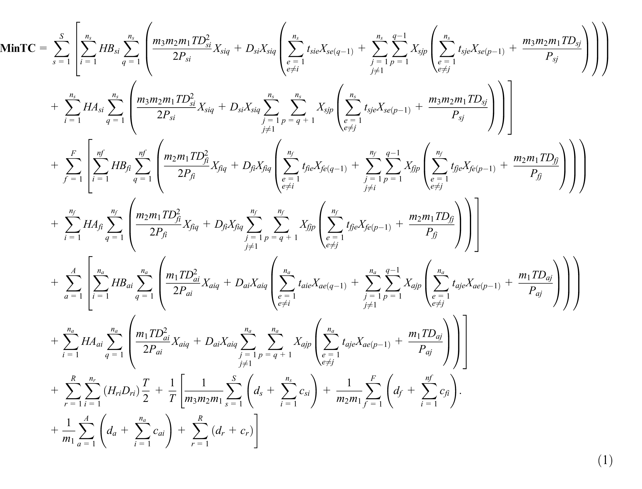
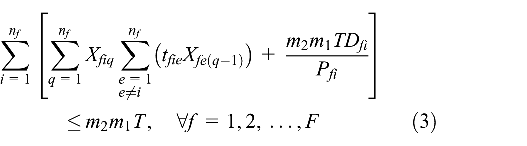
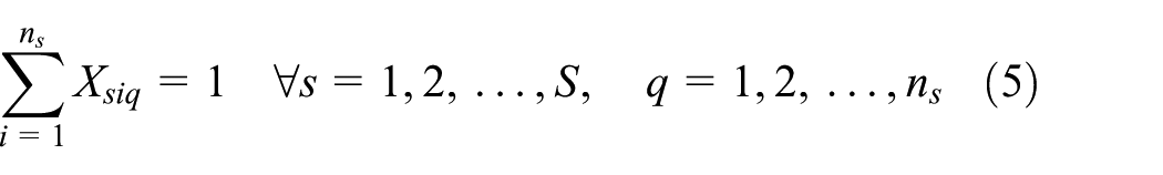
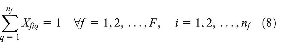
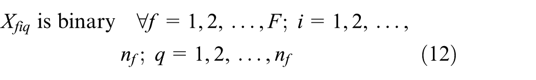
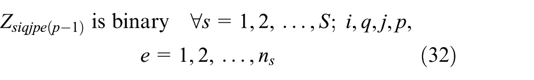
Equations (1)–(13) represent ELDSP. The objective function calculation will be explained in Appendix 1. Equations (2)–(4) ensure feasibility of cycle time under the assumption of sequence-dependent setup times, in the suppliers, fabricators, and assemblers. At the supplier stage, equations (5) and (6) guarantee assigning, in sequence, each item only to one position and each position just to one item. Equations (7)–(10) guarantee these conditions for each fabricator and assembler. Equations (11)–(13) represent binary variables

\begin{matrix} Min TC & = \sum_{s = 1}^{S} [\sum_{i = 1}^{n_{s}} H B_{si} \sum_{q = 1}^{n_{s}} (\frac{m_{3} m_{2} m_{1} {TD}_{si}^{2}}{2 P_{si}} X_{siq} + D_{si} X_{siq} (\sum_{\binom{e = 1}{e \neq i}}^{n_{s}} t_{sie} X_{se (q - 1)} + \sum_{\binom{j = 1}{j \neq 1}}^{n_{s}} \sum_{p = 1}^{q - 1} X_{sjp} (\sum_{\binom{e = 1}{e \neq j}}^{n_{s}} t_{sje} X_{se (p - 1)} + \frac{m_{3} m_{2} m_{1} T D_{sj}}{P_{sj}}))) \\ + \sum_{i = 1}^{n_{s}} H A_{si} \sum_{q = 1}^{n_{s}} (\frac{m_{3} m_{2} m_{1} {TD}_{si}^{2}}{2 P_{si}} X_{siq} + D_{si} X_{siq} \sum_{\binom{j = 1}{j \neq 1}}^{n_{s}} \sum_{p = q + 1}^{n_{s}} X_{sjp} (\sum_{\binom{e = 1}{e \neq j}}^{n_{s}} t_{sje} X_{se (p - 1)} + \frac{m_{3} m_{2} m_{1} T D_{sj}}{P_{sj}}))] \\ + \sum_{f = 1}^{F} [\sum_{i = 1}^{nf} H B_{fi} \sum_{q = 1}^{nf} (\frac{m_{2} m_{1} {TD}_{fi}^{2}}{2 P_{fi}} X_{fiq} + D_{fi} X_{fiq} (\sum_{\binom{e = 1}{e \neq i}}^{n_{f}} t_{fie} X_{fe (q - 1)} + \sum_{\binom{j = 1}{j \neq i}}^{n_{f}} \sum_{p = 1}^{q - 1} X_{fjp} (\sum_{\binom{e = 1}{e \neq j}}^{n_{f}} t_{fje} X_{fe (p - 1)} + \frac{m_{2} m_{1} T D_{fj}}{P_{fj}}))) \\ + \sum_{i = 1}^{n_{f}} H A_{fi} \sum_{q = 1}^{n_{f}} (\frac{m_{2} m_{1} {TD}_{fi}^{2}}{2 P_{fi}} X_{fiq} + D_{fi} X_{fiq} \sum_{\binom{j = 1}{j \neq 1}}^{n_{f}} \sum_{p = q + 1}^{n_{f}} X_{fjp} (\sum_{\binom{e = 1}{e \neq j}}^{n_{f}} t_{fje} X_{fe (p - 1)} + \frac{m_{2} m_{1} T D_{fj}}{P_{fj}}))] \\ + \sum_{a = 1}^{A} [\sum_{i = 1}^{n_{a}} H B_{ai} \sum_{q = 1}^{n_{a}} (\frac{m_{1} {TD}_{ai}^{2}}{2 P_{ai}} X_{aiq} + D_{ai} X_{aiq} (\sum_{\binom{e = 1}{e \neq i}}^{n_{a}} t_{aie} X_{ae (q - 1)} + \sum_{\binom{j = 1}{j \neq 1}}^{n_{a}} \sum_{p = 1}^{q - 1} X_{ajp} (\sum_{\binom{e = 1}{e \neq j}}^{n_{a}} t_{aje} X_{ae (p - 1)} + \frac{m_{1} T D_{aj}}{P_{aj}}))) \\ + \sum_{i = 1}^{n_{a}} H A_{ai} \sum_{q = 1}^{n_{a}} (\frac{m_{1} {TD}_{ai}^{2}}{2 P_{ai}} X_{aiq} + D_{ai} X_{aiq} \sum_{\binom{j = 1}{j \neq 1}}^{n_{a}} \sum_{p = q + 1}^{n_{a}} X_{ajp} (\sum_{\binom{e = 1}{e \neq j}}^{n_{a}} t_{aje} X_{ae (p - 1)} + \frac{m_{1} T D_{aj}}{P_{aj}}))] \\ + \sum_{r = 1}^{R} \sum_{i = 1}^{n_{r}} (H_{ri} D_{ri}) \frac{T}{2} + \frac{1}{T} [\frac{1}{m_{3} m_{2} m_{1}} \sum_{s = 1}^{S} (d_{s} + \sum_{i = 1}^{n_{s}} c_{si}) + \frac{1}{m_{2} m_{1}} \sum_{f = 1}^{F} (d_{f} + \sum_{i = 1}^{nf} c_{fi}) \end{matrix} + \frac{1}{m_{1}} \sum_{a = 1}^{A} (d_{a} + \sum_{i = 1}^{n_{a}} c_{ai}) + \sum_{r = 1}^{R} (d_{r} + c_{r})]

(1)

Subject to

\sum_{i = 1}^{n_{s}} [\sum_{q = 1}^{n_{s}} X_{siq} \sum_{\binom{e = 1}{e \neq i}}^{n_{s}} (t_{sie} X_{se (q - 1)}) + \frac{m_{3} m_{2} m_{1} T D_{si}}{P_{si}}] \leq m_{3} m_{2} m_{1} T, \forall s = 1, 2, \dots, S

(2)

\sum_{i = 1}^{n_{f}} [\sum_{q = 1}^{n_{f}} X_{fiq} \sum_{\binom{e = 1}{e \neq i}}^{n_{f}} (t_{fie} X_{fe (q - 1)}) + \frac{m_{2} m_{1} T D_{fi}}{P_{fi}}] \leq m_{2} m_{1} T, \forall f = 1, 2, \dots, F

(3)

\sum_{i = 1}^{n_{a}} [\sum_{q = 1}^{n_{a}} X_{aiq} \sum_{\binom{e = 1}{e \neq i}}^{n_{a}} (t_{aie} X_{ae (q - 1)}) + \frac{m_{1} T D_{ai}}{P_{ai}}] \leq m_{1} T, \forall a = 1, 2, \dots, A

(4)

\sum_{i = 1}^{n_{s}} X_{siq} = 1 \forall s = 1, 2, \dots, S, q = 1, 2, \dots, n_{s}

(5)

\sum_{q = 1}^{n_{s}} X_{siq} = 1 \forall s = 1, 2, \dots, S, i = 1, 2, \dots, n_{s}

(6)

\sum_{i = 1}^{n_{f}} X_{fiq} = 1 \forall f = 1, 2, \dots, F, q = 1, 2, \dots, n_{f}

(7)

\sum_{q = 1}^{n_{f}} X_{fiq} = 1 \forall f = 1, 2, \dots, F, i = 1, 2, \dots, n_{f}

(8)

\sum_{i = 1}^{n_{a}} X_{aiq} = 1 \forall a = 1, 2, \dots, A, q = 1, 2, \dots, n_{a}

(9)

\sum_{q = 1}^{n_{a}} X_{aiq} = 1 \forall a = 1, 2, \dots, A, i = 1, 2, \dots, n_{a}

(10)

X_{siq} is binary \forall s = 1, 2, \dots, S; i = 1, 2, \dots, n_{s}; q = 1, 2, \dots, n_{s}

(11)

X_{fiq} is binary \forall f = 1, 2, \dots, F; i = 1, 2, \dots, n_{f}; q = 1, 2, \dots, n_{f}

(12)

X_{aiq} is binary \forall a = 1, 2, \dots, A; i = 1, 2, \dots, n_{a}; q = 1, 2, \dots, n_{a}

(13)

Linearization

We consider equation (1) to linearization of the objective function. We use the Hahn et al.⁹ method to linearization type one. The auxiliary variable $Y_{fiqjp}$ is used in fabricators stage for multiplying two binary variables $X_{fiq} \times X_{fjp}$ , which have added constraints (14)–(22) to the model by applying them in the suppliers, fabricators, and assemblers stage. By the development of this method, we use a new binary variable where three binary variables multiply. For example, in the fabricators stage, $X_{fiq} \times X_{fjp} \times X_{fe (p - 1)}$ is replaced by auxiliary binary variable $Z_{fiqjpe (p - 1)}$ that by considering the suppliers, fabricators, and assemblers stage, we add constraints (23)–(34) to the model

X_{siq} = \sum_{\binom{p = 1}{p \neq q}}^{n_{s}} Y_{siqjp} \forall s = 1, 2, \dots, S; i, q, j = 1, 2, \dots, n_{s}; j \neq i

(14)

X_{fiq} = \sum_{\binom{p = 1}{p \neq q}}^{n_{f}} Y_{fiqjp} \forall f = 1, 2, \dots, F; i, q, j = 1, 2, \dots, n_{f}; j \neq i

(15)

X_{aiq} = \sum_{\binom{p = 1}{p \neq q}}^{n_{a}} Y_{aiqjp} \forall a = 1, 2, \dots, A; i, q, j = 1, 2, \dots, n_{a}; j \neq i

(16)

Y_{siqjp} = Y_{sjpiq} \forall s = 1, 2, \dots, S; i, q, j, p = 1, 2, \dots, n_{s}; i < j; q \neq p

(17)

Y_{fiqjp} = Y_{fjpiq} \forall f = 1, 2, \dots, F; i, q, j, p = 1, 2, \dots, n_{f}; i < j; q \neq p

(18)

Y_{aiqjp} = Y_{ajpiq} \forall a = 1, 2, \dots, A; i, q, j, p = 1, 2, \dots, n_{a}; i < j; q \neq p

(19)

Y_{siqjp} is binary \forall s = 1, 2, \dots, S; i, q, j, p = 1, 2, \dots, n_{s}

(20)

Y_{fiqjp} is binary \forall f = 1, 2, \dots, F; i, q, j, p = 1, 2, \dots, n_{f}

(21)

Y_{aiqjp} is binary \forall a = 1, 2, \dots, A; i, q, j, p = 1, 2, \dots, n_{a}

(22)

Y_{sjpe (p - 1)} = \sum_{\binom{q = 1}{q \neq p}}^{n_{s}} Z_{siqjpe (p - 1)} \forall s = 1, 2, \dots, S; i, j, e, p = 1, 2, \dots, n_{s}; j \neq i \neq e

(23)

Y_{fjpe (p - 1)} = \sum_{\binom{q = 1}{q \neq p}}^{n_{f}} Z_{fiqjpe (p - 1)} \forall f = 1, 2, \dots, F; i, j, e, p = 1, 2, \dots, n_{f}; j \neq i \neq e

(24)

Y_{ajpe (p - 1)} = \sum_{\binom{q = 1}{q \neq p}}^{n_{a}} Z_{aiqjpe (p - 1)} \forall a = 1, 2, \dots, A; i, j, e, p = 1, 2, \dots, n_{a}; j \neq i \neq e

(25)

X_{siq} = \sum_{\binom{p = 2}{p \neq q}}^{n_{s}} Z_{siqjpe (p - 1)} \forall s = 1, 2, \dots, S; i, q, j, e = 1, 2, \dots, n_{s}; j \neq i \neq e

(26)

X_{fiq} = \sum_{\binom{p = 2}{p \neq q}}^{n_{f}} Z_{fiqjpe (p - 1)} \forall f = 1, 2, \dots, F; i, q, j, e = 1, 2, \dots, n_{f}; j \neq i \neq e

(27)

X_{aiq} = \sum_{\binom{p = 2}{p \neq q}}^{n_{a}} Z_{aiqjpe (p - 1)} \forall a = 1, 2, \dots, A; i, q, j, e = 1, 2, \dots, n_{a}; j \neq i \neq e

(28)

Z_{siqjpe (p - 1)} = Z_{sjpe (p - 1) iq} \forall s = 1, 2, \dots, S; i, q, j, p, e = 1, 2, \dots, n_{s}; i < j < e; q \neq p

(29)

Z_{fiqjpe (p - 1)} = Z_{fjpe (p - 1) iq} \forall f = 1, 2, \dots, F; i, q, j, p, e = 1, 2, \dots, n_{f}; i < j < e; q \neq p

(30)

Z_{aiqjpe (p - 1)} = Z_{ajpe (p - 1) iq} \forall a = 1, 2, \dots, A; i, q, j, p, e = 1, 2, \dots, n_{a}; i < j < e; q \neq p

(31)

Z_{siqjpe (p - 1)} is binary \forall s = 1, 2, \dots, S; i, q, j, p, e = 1, 2, \dots, n_{s}

(32)

Z_{fiqjpe (p - 1)} is binary \forall f = 1, 2, \dots, F; i, q, j, p, e = 1, 2, \dots, n_{f}

(33)

Z_{aiqjpe (p - 1)} is binary \forall a = 1, 2, \dots, A; i, q, j, p, e = 1, 2, \dots, n_{a}

(34)

We use the Adams and Forrester¹⁰ method for linearization of multiplying continuous variable T by one binary variable. For example, we replace $X_{fiq} \times T$ by $V_{fiq} + L X_{fiq}$ terms in the fabricators stage where L and U are the lower and upper bounds of continuous variable T, respectively, and $V_{fiq}$ is the non-negative continuous variable. Therefore, we add constraints (35)–(40) to the model for suppliers, fabricators, and assemblers stage. But continuous variable is multiplied by the product of two binary variables in equation (1). For example, in fabricators stage, we have $X_{fiq} \times X_{fjp} \times T$ , considering linearization of the product of two variables $X_{fiq} \times X_{fjp}$ that replaces by auxiliary binary variable. We can replace $Y_{fiqjp} \times T$ by $W_{fiqjp} + L Y_{fiqjp}$ with linearization development,¹⁰ where L and U are the lower and upper bound of continuous variable T, respectively. $W_{fiqjp}$ is the non-negative continuous variable. For this type of linearization, by considering suppliers, fabricators, and assemblers stage, we add equations (41)–(46) to the model

V_{siq} \geq T - U (1 - X_{siq}) - L X_{siq} \forall s = 1, 2, \dots, S; i, q = 1, 2, \dots, n_{s}

(35)

V_{fiq} \geq T - U (1 - X_{fiq}) - L X_{fiq} \forall f = 1, 2, \dots, F; i, q = 1, 2, \dots, n_{f}

(36)

V_{aiq} \geq T - U (1 - X_{aiq}) - L X_{aiq} \forall a = 1, 2, \dots, A; i, q = 1, 2, \dots, n_{a}

(37)

V_{siq} \geq 0 \forall s = 1, 2, \dots, S; i, q = 1, 2, \dots, n_{s}

(38)

V_{fiq} \geq 0 \forall f = 1, 2, \dots, F; i, q = 1, 2, \dots, n_{f}

(39)

V_{aiq} \geq 0 \forall a = 1, 2, \dots, A; i, q = 1, 2, \dots, n_{a}

(40)

W_{siqjp} \geq T - U (1 - Y_{siqjp}) - L Y_{siqjp} \forall s = 1, 2, \dots, S; i, q, j, p = 1, 2, \dots, n_{s}; i \neq j; q \neq p

(41)

W_{fiqjp} \geq T - U (1 - Y_{fiqjp}) - L Y_{fiqjp} \forall f = 1, 2, \dots, F; i, q, j, p = 1, 2, \dots, n_{f}; i \neq j; q \neq p

(42)

W_{aiqjp} \geq T - U (1 - Y_{aiqjp}) - L Y_{aiqjp} \forall a = 1, 2, \dots, A; i, q, j, p = 1, 2, \dots, n_{a}; i \neq j; q \neq p

(43)

W_{siqjp} \geq 0 \forall s = 1, 2, \dots, S; i, q, j, p = 1, 2, \dots, n_{s}

(44)

W_{fiqjp} \geq 0 \forall f = 1, 2, \dots, F; i, q, j, p = 1, 2, \dots, n_{f}

(45)

W_{aiqjp} \geq 0 \forall a = 1, 2, \dots, A; i, q, j, p = 1, 2, \dots, n_{a}

(46)

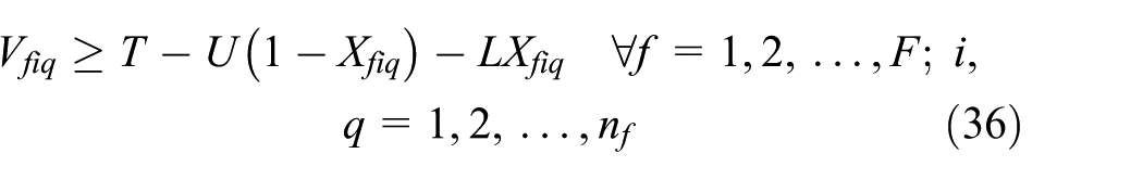
Equation (1), with making these changes, becomes equation (50). In equation (50), L the lower bound of variable T is equal to the minimum value that satisfies equations (47)–(49) and U the upper bound of variable T is equal to planning horizon time

\sum_{i = 1}^{n_{s}} [\sum_{q = 1}^{n_{s}} \sum_{\binom{e = 1}{e \neq i}}^{n_{s}} (t_{sie} Y_{siqe (q - 1)}) + \frac{m_{3} m_{2} m_{1} T D_{si}}{P_{si}}] \leq m_{3} m_{2} m_{1} T \forall s = 1, 2, \dots, S

(47)

\sum_{i = 1}^{n_{f}} [\sum_{q = 1}^{n_{f}} \sum_{\binom{e = 1}{e \neq i}}^{n_{f}} (t_{fie} Y_{fiqe (q - 1)}) + \frac{m_{2} m_{1} T D_{fi}}{P_{fi}}] \leq m_{2} m_{1} T \forall f = 1, 2, \dots, F

(48)

\sum_{i = 1}^{n_{a}} [\sum_{q = 1}^{n_{a}} \sum_{q = 1}^{n_{a}} \sum_{\binom{e = 1}{e \neq i}}^{n_{a}} (t_{aie} Y_{aiqe (q - 1)}) + \frac{m_{1} T D_{ai}}{P_{ai}}] \leq m_{1} T \forall a = 1, 2, \dots, A

(49)

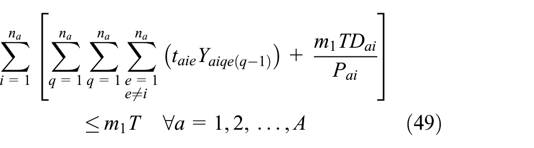
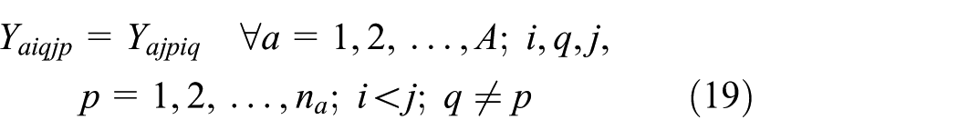
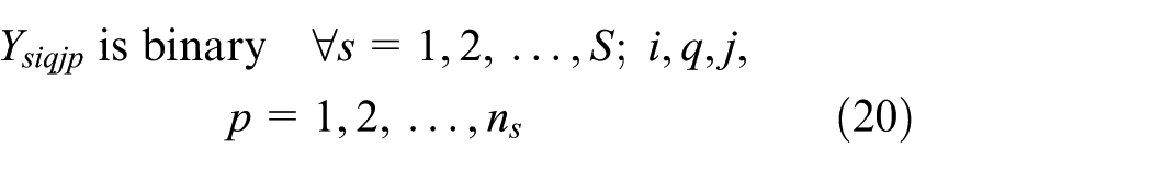
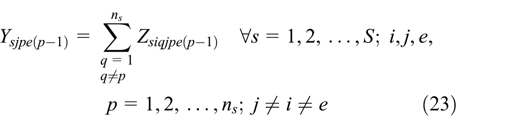
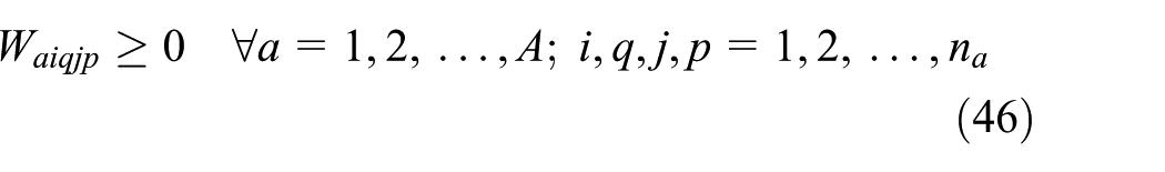
After linearization, we represent the original objective function by equation (50). The linearized model includes two sets of new equations: equations (14)–(34) and equations (35)–(46), and also equations (5)–(13) belong to the original model. Furthermore, because of linearization, we replace equations (2)–(4) by equations (47)–(49)

\begin{matrix} M i n T C = \sum_{S = 1}^{S} [\sum_{i = 1}^{n_{s}} H B_{s i} \sum_{q = 1}^{n_{s}} (\frac{m_{3} m_{2} m_{1} D_{s i}^{2}}{2 P_{s i}} (V_{s i q} + L X_{s i q}) + D_{s i} (\sum_{\begin{array}{l} e = 1 \\ e \neq i \end{array}}^{n_{s}} t_{s i e} Y_{s i q e (q - 1)} + \sum_{\begin{array}{l} j = 1 \\ j \neq i \end{array}}^{n_{s}} \sum_{p = 1}^{q - 1} (\sum_{\begin{array}{l} e = 1 \\ e \neq j \end{array}}^{n_{s}} t_{s j e} Z_{s i q j p e (p - 1)} + \frac{m_{3} m_{2} m_{1} D_{s j}}{P_{s j}} (W_{s i q j p} + L Y_{s i q j p})))) \\ + \sum_{i = 1}^{n_{s}} H A_{s i} \sum_{q = 1}^{n_{s}} (\frac{m_{3} m_{2} m_{1} D_{s i}^{2}}{2 P_{s i}} (V_{s i q} + L X_{s i q}) + D_{s i} \sum_{\begin{array}{l} j = 1 \\ j \neq i \end{array}}^{n_{s}} \sum_{p = q + 1}^{n_{s}} (\sum_{\begin{array}{l} e = 1 \\ e \neq j \end{array}}^{n_{s}} t_{s j e} Z_{s i q j p e (p - 1)} + \frac{m_{3} m_{2} m_{1} D_{s j}}{P_{s j}} (W_{s i q j p} + L Y_{s i q j p})))] \\ + \sum_{i = 1}^{F} [\sum_{i = 1}^{n_{f}} H B_{f i} \sum_{q = 1}^{n_{f}} (\frac{m_{2} m_{1} D_{f i}^{2}}{2 P_{f i}} (V_{f i q} + L X_{f i q}) + D_{f i} (\sum_{\begin{array}{l} e = 1 \\ e \neq i \end{array}}^{n_{f}} t_{f i e} Y_{f i q e (q - 1)} + \sum_{\begin{array}{l} j = 1 \\ j \neq i \end{array}}^{n_{f}} \sum_{p = 1}^{q - 1} (\sum_{\begin{array}{l} e = 1 \\ e \neq j \end{array}}^{n_{f}} t_{f j e} Z_{f i q j p e (p - 1)} + \frac{m_{2} m_{1} D_{f j}}{P_{f j}} (W_{f i q j p} + L Y_{f i q j p})))) \\ + \sum_{i = 1}^{n_{f}} H A_{f i} \sum_{q = 1}^{n_{f}} (\frac{m_{2} m_{1} D_{f i}^{2}}{2 P_{f i}} (V_{f i q} + L X_{f i q}) + D_{f i} \sum_{\begin{array}{l} j = 1 \\ j \neq i \end{array}}^{n_{f}} \sum_{p = q + 1}^{n_{f}} (\sum_{\begin{array}{l} e = 1 \\ e \neq j \end{array}}^{n_{f}} t_{f j e} Z_{f i q j p e (p - 1)} + \frac{m_{2} m_{1} D_{f j}}{P_{f j}} (W_{f i q j p} + L Y_{f i q j p})))] \\ + \sum_{a = 1}^{A} [\sum_{i = 1}^{n_{a}} H B_{a i} \sum_{q = 1}^{n_{a}} (\frac{m_{1} D_{a i}^{2}}{2 P_{a i}} (V_{a i q} + L X_{a i q}) + D_{a i} (\sum_{\begin{array}{l} e = 1 \\ e \neq i \end{array}}^{n_{a}} t_{a i e} Y_{a i q e (q - 1)} + \sum_{\begin{array}{l} j = 1 \\ j \neq i \end{array}}^{n_{a}} \sum_{p = 1}^{q - 1} (\sum_{\begin{array}{l} e = 1 \\ e \neq j \end{array}}^{n_{a}} t_{a j e} Z_{a i q j p e (p - 1)} + \frac{m_{1} D_{a j}}{P_{a j}} (W_{a i q j p} + L Y_{a i q j p})))) \\ + \sum_{i = 1}^{n_{a}} H A_{a i} \sum_{q = 1}^{n_{a}} (\frac{m_{1} D_{a i}^{2}}{2 P_{a i}} (V_{a i q} + L X_{a i q}) + D_{a i} \sum_{\begin{array}{l} j = 1 \\ j \neq i \end{array}}^{n_{a}} \sum_{p = q + 1}^{n_{a}} (\sum_{\begin{array}{l} e = 1 \\ e \neq j \end{array}}^{n_{a}} t_{a j e} Z_{a i q j p e (p - 1)} + \frac{m_{1} D_{a j}}{P_{a j}} (W_{a i q j p} + L Y_{a i q j p})))] \\ + \sum_{r = 1}^{R} \sum_{i = 1}^{n_{r}} (H_{r i} D_{r i}) \frac{T}{2} + \frac{1}{T} [\frac{1}{m_{3} m_{2} m_{1}} \sum_{s = 1}^{S} (d_{s} + \sum_{i = 1}^{n_{s}} c_{s i}) + \frac{1}{m_{2} m_{1}} \sum_{f = 1}^{F} (d_{f} + \sum_{i = 1}^{n_{f}} c_{f i}) + \frac{1}{m_{1}} \sum_{a = 1}^{A} (d_{a} + \sum_{i = 1}^{n_{a}} c_{a i}) + \sum_{r = 1}^{R} (d_{r} + c_{r})] \end{matrix}

(50)

subject to equations (5)–(49).

Proposed algorithms

Imperialist competitive algorithm

One of the novel socio-politically evolutionary algorithms that has been presented for treating with several optimization problems recently is an imperialist competitive algorithm (ICA).¹¹ The suitable performance and applicability of the algorithm in both convergence rate and achieving near optimal solutions are the advantages of the ICA.¹² The algorithm commences with an initial population and each individual of the population is called a country.¹³

At first, the imperialist states are created by some of the best countries, then the remainder of the countries organize the colonies of these imperialists. In other words, all the colonies of initial population are divided among the mentioned imperialists based on their power. The power of each country has an inverse relation with its cost in the objective function. The imperialist states and their colonies establish some empires.^13,14 The total power of an empire is calculated by the sum of the total power of imperialist country and a percentage of mean power of its colonies. The colonies of each empire start to approach the related imperialist country, after constructing the primary empires.¹⁴Figure 1 shows flow chart of ICA.

Figure 1.

Flow chart of ICA.

The ICA is explained in the following subsections.

Solution representation

The representation of a solution is one of the most important parts of a meta-heuristic design to provide efficient search of the space. There are two different representations in the literature.^15,16 We used one of them.¹⁵ We have two suppliers (suppliers 1 and 2), one fabricator (fabricator 1), and two assemblers (assemblers 1 and 2), whereas those that are used in the previous literature are 6 and 4, 5 and 4, and 5 items, respectively. In Figure 2, the code of the individual corresponding solutions is 3-5-4-2-1-6 at supplier 1, 1-3-2-4 at supplier 2, 5-4-1-2-3 at single fabricator, 1-3-4-2 at assembler 1, and 2-1-4-3-5 at assembler2.

Figure 2.

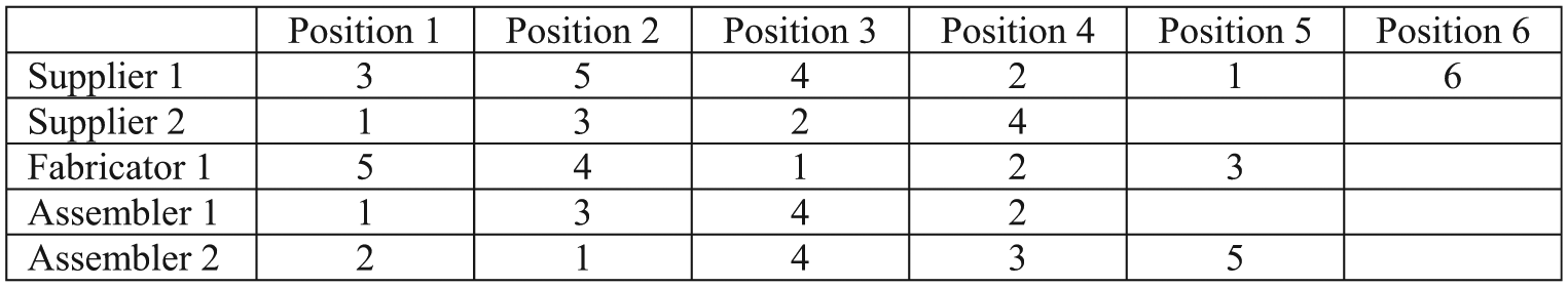
A sample chromosome.

Generating initial empires

Each evolutionary algorithm starts with an initial solution. To form the initial solution, an array of variable values is created. The array is called “country” in the ICA. In an N-dimensional problem, a country is presented by a 1 × N array. The mentioned array is defined by

Country = [P_{1}, P_{2}, \dots ., P_{N}]

(51)

The cost of a country is gained by defining the objective function TC at the variables (P₁, P₂, …, P_N). Then, the cost of a country is calculated by

TC (Country) = TC (P_{1}, P_{2}, \dots, P_{N})

(52)

The optimization procedure is started by generating an initial population of size $N_{pop}$ and then $N_{imp}$ of the most powerful countries are selected to form imperialists. $N_{col} (N_{col} = N_{pop} - N_{imp})$ of the initial population is remained, which form the colonies of these empires and each of the colonies belongs to an empire. Now the initial population is divided into two groups, namely, imperialist and colony. Based on the power of each colony, they are distributed among the imperialists. To proportionally divide the colonies between imperialists, the normalized cost of an empire is calculated by

{\bar{TC}}_{n} = T C_{n} - max_{i} {T C_{i}}, i = 1, 2, \dots, N_{imp}

(53)

where TC_n is the TC of the nth imperialist and ${\bar{TC}}_{n}$ is its normalized TC. Considering the ${\bar{TC}}_{n}$ of all imperialists, the normalized power of each imperialist can be calculated as follows

p_{n} = | \frac{T C_{n}}{\sum_{i = 1}^{N_{imp}} T C_{i}} |

(54)

The normalized power of each imperialist will affect on the number of colonies that belong to that empire. To calculate the initial number of colonies of the nth empire, the following relation can be considered

NT C_{n} = round {p_{n} \times N_{col}}

(55)

where $NT C_{n}$ is the number of colonies of the nth empire and $N_{col}$ is the total number of initial colonies. $NT C_{n}$ of the colonies are randomly selected and assigned to the nth imperialist to distribute the colonies. The nth empire is formed by the mentioned colonies and the nth imperialist. Consequently, the stronger empires have more colonies, while the weaker ones have less.^13,14

Searching space

Three steps (assimilation, crossover, and revolution) are used to find a better solution during the search process. Those steps are described as follows.

Assimilation

In the ICA, the uniformity of colonies culture and social structure toward their imperialist is achieved by the assimilation policy. In this step, the colony moves toward the imperialist by x units, in which x is a random variable with a uniform distribution

x ~ U (0, ϑ \times d), ϑ > 1

(56)

where d is the distance among colonies and imperialist. $ϑ > 1$ causes the colony to come near to the imperialist country from both sides. The vector that connects the colony to imperialist is the main direction of the movement. So $θ$ angle is added to this direction to search various directions around the imperialist and a wider area around the current solution

θ ~ U (- Θ, Θ)

(57)

where $θ$ is a random number and $Θ$ is a parameter that adjusts the amount of deviation from the original path (Figure 3). It is approximated that a value of 2 for $ϑ$ and $π / 4$ for $Θ$ is the most proper value.^13,14

Figure 3.

Movement of colony toward their relevant imperialist.

Crossover

Using the crossover operator in this step, the colonies share their information with each other to modify themselves. Colonies with lower cost have more opportunity for sharing their information under a binary tournament selection. Three various kinds of crossover operators (one point, two points, and uniform crossover) are adapted to encoded parts of solutions.¹⁷

Revolution

Revolution is defined as a basic and sudden change in the power structure and sociopolitical characteristics of a country. Instead of being assimilated by an imperialist, the position of the colony is randomly changed in the sociopolitical direction. The advantages of revolution can be considered as follows: (1) increasing the search of the algorithm in solution space and (2) preventing the early convergence of countries to local minimums. The percentage of the colonies in each colony which will randomly change their position is defined as the revolution rate. A very high value of a revolution will result in decreasing the exploitative power of algorithm and can reduce its convergence rate.^13,18 In this article, three kinds of revolution strategy are applied to the encoded parts of solutions, consisting of (1) swap, (2) reversion, and (3) inversion. For more details, see Mohammadi et al.¹⁷

Exchange positions of the imperialist and a colony

Moving toward the imperialist, the position of the imperialist and the colony is exchanged if a colony reaches to a position with a lower cost than the expense of the imperialist. Then, the ICA is kept by the new imperialist and the colonies move toward the new imperialist in the new position.^13,14,18

Uniting similar empires

Some imperialists might be situated on the same positions. The integration of these empires will form a new empire if the distance between the two imperialists becomes less than threshold distance. The colonies of the new empire are established by all the colonies of two empires and one of the two imperialists will be chosen as the new imperialist.^13,18

Total power of an empire

The power of an imperialist and its colonies are the two influential factors in calculating the total power of an empire. But the imperialist power is the main power in one empire. Therefore, the total cost (TTC) of the nth empire is computed by

TT C_{n} = TC (imperialis t_{n}) + ε . Mean {TC (coloniesofempir e_{n})}

(58)

where TTC_n is the total cost of the nth empire and $ε$ is a small positive number. Small values for $ε$ will cause the total power of the empire to be formed by just the power of the imperialist and increasing it, while large values will lead to increasing the effectiveness of the colonies in calculating the total power of an empire. The value of 0.1 for $ε$ is an acceptable value.^13,18

Imperialistic competition

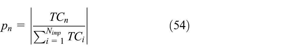
In the ICA, each empire attempts to take possession of colonies of other empires. Finally, the power of stronger empires will be increased and the power of weaker ones will be decreased or they will be eliminated. The power of each empire plays an important role in succeeding in this competition. Therefore, the stronger empires have greater opportunity to take possession of the weakest countries in weakest empires. In other words, these colonies may not be possessed by the strongest empire, but this empire will own it with a higher probability. The possession probability of each empire is computed based on its total power. Normalized total cost of nth empire is obtained by

{\bar{TTC}}_{n} = TT C_{n} - max_{i} {TT C_{i}}, i = 1, 2, \dots, N_{imp}

(59)

where ${\bar{TTC}}_{n}$ and $TT C_{n}$ are the normalized total cost and total cost of the nth empire, respectively. Considering the normalized total cost of an empire, the possession probability of each empire is defined by

p_{p_{n}} = | \frac{{\bar{TTC}}_{n}}{\sum_{i = 1}^{N_{imp}} {\bar{TTC}}_{i}} |

(60)

To distribute the colonies among empires according to the possession probability of them, a new procedure with less computational stages is used rather than simple Rolette Wheel selection. At the beginning, vector P is formed as

P = [p_{p_{1}}, p_{p_{2}}, \dots, p_{p_{N_{imp}}}]

(61)

Then a vector R with the same size as P is made and its elements are random numbers uniformly distributed between 0 and 1

R = [r_{1}, r_{2}, \dots, r_{N_{imp}}]; r_{1}, r_{2}, \dots, r_{N_{imp}} ~ U (0, 1)

(62)

Then, vector D is created by subtracting R from P

D = P - R = [D_{1}, D_{2}, \dots, D_{N_{imp}}] = [p_{p_{1}} - r_{1}, p_{p_{2}} - r_{2}, \dots, p_{p_{N_{imp}}} - r_{N_{imp}}]

(63)

Referring to vector D , the forgoing colony is handed to an empire with the highest relevant index value in D .¹²

Eliminating the powerless empires

When the weak empire loses all its colonies, the empire collapse and the colonies of that empire are distributed among the other stronger empires.¹⁸

Convergence

Finally, the imperialistic competition ends (stop condition) if all the colonies will be under the control of most powerful empire and other empires will collapse.^12,18

Modified ICA

In the general ICA, the uniformity of colonies culture and social structure toward their imperialist is achieved by the assimilation policy. Moreover, in the real world, the imperialist countries will also move toward the most powerful imperialist countries which they realize themselves weak or even the associated imperialists will outdistance the greater imperialist.

Figure 4 shows this modification of ICA (MCIA). The $d'$ is the distance among imperialist countries and strongest imperialist. The imperialist countries move toward the strongest imperialist by random value $(x')$ and random angle $(θ')$ , in which $x'$ and $θ^{'}$ are a random variable with a uniform distribution

x' ~ U (0, ϑ' \times d')

(64)

θ' ~ U (- Θ', Θ')

(65)

The act $ϑ'$ and $Θ'$ like the $ϑ$ and $Θ$ . This movement will take place if the new position provides more power to the imperialist country Otherwise, the imperialist will keep its previous position.

Figure 4.

Movement of imperialist country toward stronger imperialist.

Figure 5 shows the new assimilation policy, in which first imperialists move toward the strongest imperialist to increase their power, and then colonies will pull to their imperialists.

Figure 5.

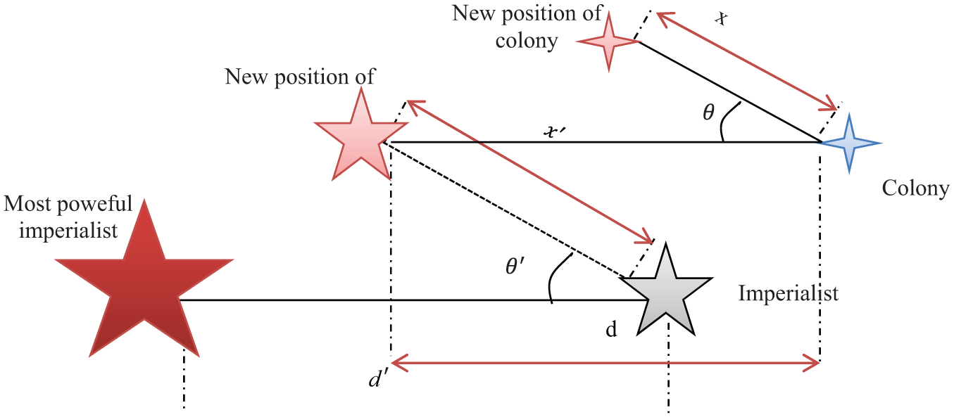
The mechanism of assimilation policy in MICA.

Teaching learning–based optimization

A nature-inspired algorithm which is a population-based technique known as “teaching learning–based optimization” (TLBO). In TLBO, a population of solutions as learners is used to reach the global solution based on the effect of the instruction of teacher on the learner’s grade that is equivalent to the “fitness” value of the optimization problem. The teacher is examined as the best solution obtained so far.¹⁹

The procedure of TLBO is divided into two phase: (1) teacher phase, which is learning from teacher and (2) learning phase, which is learning through interchange of information between learners. These phases are described as follows.

Teacher phase

In this phase, the teacher position is allocated to the best individual $(X_{teacher})$ in the population, then learners or other individuals (X_i) are proceeded by shifting their positions toward the teacher’s position X_teacher.

The position of each individual (X_i) solution is improved, as X_new, according to the difference between the current and the new mean value as follows

X_{new} = X_{i} + Rand (0, 1) \times (X_{teacher} - T_{F} X_{Mean})

(66)

where $Rand (0, 1)$ is a random number in the range [0, 1], X_teacher will be designated as the new mean value in next generation, $X_{Mean}$ is the mean value of the individuals in current generation, $T_{F}$ is a teaching factor that controls the value of the mean to be changed. The $T_{F}$ can be either 1 or 2 which is again a heuristic step and decided randomly with equal probability as

T_{F} = Round [1 + Rand (0, 1) \times (2 - 1)]

(67)

Learner phase

In this phase, self-organized learning between the individual $(X_{i}$ ) and other learners $(X_{j})$ is increased the knowledge of an individual, where obviously, i is not equal to j. Two situations can happen based on the knowledge levels of these two individuals relative to each other. If $X_{j}$ is better than $X_{i}$ , then $X_{i}$ will be moved toward $X_{j}$ (i.e. equation (68)) and otherwise, it will be moved from $X_{j}$ (i.e. equation (69))

X_{new} = X_{i} + Rand (0, 1) \times (X_{j} - X_{i})

(68)

X_{new} = X_{i} + Rand (0, 1) \times (X_{i} - X_{j})

(69)

At the end, $X_{new}$ will be accepted into the population if it achieves better performance. The termination criterion will be satisfied if the number of generations reach to the maximum number of generations. Figure 6 shows a flow chart of TLBO Algorithm.

Figure 6.

Flow chart of TLBO algorithm.

Hybrid MICA–TLBO

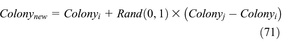
We propose a hybrid algorithm including MICA and TLBO technique (MCIA–TLBO) to solve defined problem in the common cycle time and integer multipliers policy. We use TLBO to increase convergence rate and improve the final response of MICA. Figure 7 shows a flow chart of teaching and learning phases for MICA-TLBO. In each empire, imperialist plays the role of teacher and its colonies are considered as students. In teacher phase, the imperialist improves its colonies based on equation (70). In learner phase, two colonies of the same imperialist randomly select to increase the power of colonies and improve. According to which one is better than another, equation (71) or (72) can be obtained

Colon y_{new} = Colon y_{i} + Rand (0, 1) \times (Imperialis t_{teacher} - T_{F \times} Empir e_{Mean})

(70)

Colon y_{new} = Colon y_{i} + Rand (0, 1) \times (Colon y_{j} - Colon y_{i})

(71)

Colon y_{new} = Colon y_{i} + Rand (0, 1) \times (Colon y_{i} - Colon y_{j})

(72)

Figure 7.

Flow chart of teaching and learning phase for MICA–TLBO.

The two colonies will switch their positions if a colony reaches a better position than its imperialist. In MICA-TLBO, the solution time is decreased by increasing power of each empire and improving the position of imperialist and colonies. Hence, the convergence rate of the MICA-TLBO in comparison with ICA and TLBO is higher, which is shown in the results section. Figure 8 represents the flow chart of the proposed MICA-TLBO.

Figure 8.

Flow chart of MICA–TLBO.

Computational results

As shown in Table 1, 15 instances that have a different configuration and size of supply chain are presented to evaluate the proposed algorithms. For each instance, 10 problems are randomly generated and the average of the results is calculated.

Table 1.

The configuration of supply chain for instance problems.

No.	Supply chain configuration	$n_{s}$	$n_{f}$	$n_{a}$	$n_{r}$	Number of variables	Number of constraints
1	1×1×1×1	2	2	2	2	315	273
2	1×1×1×1	5	5	5	5	50,778	17,883
3	2×2×2×1	4, 2	5, 2	3, 5	4	39,610	14,754
4	3×2×3×2	6, 1, 2	8, 7	4, 2, 5	3, 3	464,114	106,262
5	3×3×3×3	3, 2, 3	2, 3, 2	4, 2, 3	3, 3, 3	592,103	137,933
6	4×3×4×3	3, 5, 3, 2	3, 7, 3	5, 3, 5, 4	4, 4, 4	385,062	102,129
7	4×4×4×4	6, 7, 4, 8	4, 6, 8, 9	2, 5, 8, 1	3, 4, 3, 4	1,554,407	314,002
8	5×5×5×4	9, 3, 5, 6, 4	6, 7, 3, 2, 8	3, 6, 7, 8, 1	2, 3, 4, 5	1,802,680	380,437
9	6×4×3×3	7, 5, 8, 9, 10, 2	2, 3, 6, 7	3, 5, 2	3, 3, 3	1,268,139	265,533
10	3×4×6×4	5, 8, 4	5, 6, 2, 3	9, 3, 5, 6, 8, 7	4, 5, 4, 5	2,850,329	520,895
11	7×6×7×4	4, 6, 8, 5, 9, 1, 4	3, 5, 2, 1, 8, 6	8, 5, 6, 2, 1, 3, 9	5, 5, 5, 5	2,110,901	422,022
12	8×8×8×6	4, 5, 8, 6, 4, 3, 5, 8	4, 6, 1, 2, 4, 7, 8, 4	4, 2, 4, 8, 9, 10, 2, 1	5, 6, 5, 6, 5, 6	4,721,938	921,150
13	10×3×5×7	3, 5, 3, 6, 9, 1, 2, 2, 1, 3	14, 12, 19	5, 12, 11, 8, 6	5, 6, 7, 2, 1, 4, 4	1,693,421	342,012
14	6×7×3×6	6, 18, 5, 9, 11, 4	6, 8, 17, 5, 6, 12, 3	14, 7, 15	7, 6, 2, 3, 1, 4	2,138,363	440,825
15	10×10×10×10	7, 5, 3, 6, 9, 1, 2, 2, 1, 3	9, 5, 8, 9, 1, 2, 9, 3, 5, 7	2, 4, 9, 6, 3, 3, 5, 2, 8, 1	3, 4, 5, 3, 2, 6, 8, 5, 4, 2	5,576,079	1,069,616

The results of computational experiments for the common cycle time and integer multipliers policies are described in two next subsections. The results are achieved on the laptop with an Intel (R) core (TM) 2-2.00 GHz CPU and 2G RAM.

The results of common cycle time policy

In the common cycle time policy, we propose MICA–TLBO and it is compared with GA relative to the solution time and solution quality. Furthermore, we adapt a hybrid algorithm (HA) which proposed by the Clausen and Ju⁵. The results represented by Table 2.

Table 2.

The results of computational experiments for the common cycle time policy.

Instance	HA	GA		ICA		MICA		MICA–TLBO
Instance	Ave. CPU time (min)	RPD	Ave. CPU time (s)	RPD	Ave. CPU time (s)	RPD	Ave. CPU time (s)	RPD	Ave. CPU time (s)
1	0.05	3.70	0.60	3.31	0.43	2.61	0.32	2.22	0.28
2	1.33	5.65	2.55	4.25	2.25	3.06	1.51	2.51	1.27
3	0.98	3.78	1.89	2.94	1.21	2	0.79	1.6	0.64
4	10.04	8.03	17.62	6.67	16.99	4.34	10.53	3.86	8.53
5	12.63	4.02	2.96	3.22	2.56	2.51	1.92	2.08	1.56
6	9.79	7.00	22.10	5.49	21.93	4.23	14.47	3.51	12.15
7	69.48	5.89	20.07	4.80	20.43	2.98	12.87	2.65	10.42
8	76.99	11.52	38.09	8.58	36.82	5.41	22.46	4.71	18.87
9	47.21	4.81	15.97	4.07	14.43	2.77	9.67	2.22	8.61
10	>120	9.67	52.45	7.65	45.93	5.13	35.37	4.57	30.77
11	>120	9.31	25.03	7.00	22.08	5.32	13.91	4.73	12.52
12	>120	12.37	104.14	10.36	89.89	8.29	62.92	6.71	54.74
13	>120	8.55	37.51	6.63	33.83	5.17	23.34	4.6	21.01
14	>120	11.29	143.64	8.90	124.45	6.68	90.85	5.95	75.41
15	>120	12.13	218.97	10.21	167.38	7.15	132.23	6.22	108.43

HA: hybrid algorithm; CPU: central processing unit; GA: genetic algorithm; ICA: imperialist competitive algorithm; MICA: modified imperialist competitive algorithm; MICA–TLBO: modified imperialist competitive algorithm and teaching learning–based optimization; RPD: relative percentage deviation.

In HA, we obtain the optimal solution with the different average solution times (ASTs; Ave. CPU time) in each instance. As shown in the second column of Table 2, ASTs are severely increased with problem size and after ninth instance, the ASTs are >120 min. The AST is very high in HA, so we proposed hybrid algorithm. We calculate the relative percentage deviation (RPD) as solution quality. Let $T C_{Algorithm}$ denotes the average total cost obtained from GA, ICA, MICA and MICA–TLBO. $T C_{Best}$ is the best known solution obtained from each instance by each algorithm. So equation (73) can calculate solution quality as follows

R P D = \frac{T C_{A l g o r i t h m} - T C_{B e s t}}{T C_{B e s t}} \times 100 %

(73)

As shown in Figure 9 and 10, the results of MICA–TLBO outperform other algorithms relative to RPD and AST in all instances.

Figure 9.

The results of RPD values for common cycle time policy in each algorithm.

Figure 10.

The average CPU time for common cycle time policy in each algorithm.

The maximum value of AST is obtained from 15th instance. In 15th instance, maximum and minimum value are 218.97 in GA and 108.43 s in MICA–TLBO, respectively. Figure 11 illustrates the convergence of the algorithms for the objective function in 15th instance. As shown in this figure, the convergence rate of the proposed algorithm, that is, MICA–TLBO, is better than other algorithms.

Figure 11.

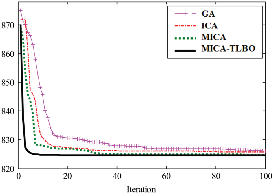
Convergence of algorithms for common cycle time policy in 15th instance.

The result of integer multipliers policy

The results of applying the integer multipliers policy are shown in Table 3. Also, it is observed from Figure 12 and 13 that the MICA–TLBO algorithm is effective in comparison to the others relative to RPD and AST.

Table 3.

The results of computational experiments for the integer multipliers policy.

Instance	GA		ICA		MICA		MICA–TLBO		Comparison between common cycle time and integer multipliers policy (% cost saving)
Instance	RPD	Ave CPU time (s)	RPD	Ave CPU time (s)	RPD	Ave CPU time (s)	RPD	Ave CPU time (s)
1	3.1	0.65	2.92	0.37	1.78	0.24	1.57	0.2	20.8
2	4.44	2.35	3.44	4.66	2.58	2.33	2.17	2.16	29.4
3	2.97	1.13	2.32	0.42	1.42	0.32	1.14	0.27	13.4
4	6.12	11.12	5.2	19.73	4.11	10.06	3.29	8.85	16.2
5	3.32	2.03	2.85	4.19	1.97	2.02	1.69	1.92	2.6
6	5.34	20.19	4.43	25.01	3.41	15.01	3.07	12.61	11.1
7	4.87	21.07	3.88	28.43	2.83	17.06	2.35	13.99	10.7
8	8.18	38.89	6.28	33.89	4.58	26.77	3.98	21.68	27.9
9	3.73	14.54	3.32	17.03	2.59	7.15	2.33	6.29	21.7
10	7.17	55.04	5.97	52.94	4.3	35.47	3.83	31.21	31.2
11	6.93	29.48	5.51	25.48	3.47	17.84	2.88	14.81	28.4
12	8.99	114.23	7.86	108.78	5.11	70.71	4.39	62.93	17.4
13	6.35	39.14	5.18	37.01	3.37	29.61	2.86	24.87	28.8
14	8.18	159.43	6.75	149.32	5.4	106.02	4.54	92.24	19.6
15	8.8	241.23	7.82	202.68	4.77	158.09	4.29	135.96	22.7

GA: genetic algorithm; ICA: imperialist competitive algorithm; MICA: modified imperialist competitive algorithm; MICA–TLBO: modified imperialist competitive algorithm and teaching learning–based optimization; RPD: relative percentage deviation; CPU: central processing unit.

Figure 12.

The results of RPD values for integer multipliers policy in each algorithm.

Figure 13.

The average CPU time for integer multipliers policy in each algorithm.

The maximum value of AST is obtained from 15th instance. In 15th instance, maximum and minimum value are 241.23 in GA and 135.96 s in MICA–TLBO, respectively. As shown in Figure 14, the convergence rate of MICA–TLBO is higher than other ones.

Figure 14.

Convergence of algorithms for integer multipliers policy in 15th instance.

The last column of Table 3 demonstrates the percentage of cost savings attained by applying the integer multipliers policy. The maximum percentage of cost savings is observed in 31.2%, which is obtained from the 10th instance. As shown in this table, the integer multipliers policy outperforms the common cycle time policy in all instances.

Conclusion

In this article, we investigate a four-stage supply chain including suppliers, fabricators, assemblers and retailers. The common cycle time and integer multipliers policies are used to synchronize the chain. We have developed a new MINLP model with objective function of minimizing inventory, transportation and production setup costs. After linearization of the model, we propose a hybrid MICA–TLBO for defined problem. The hybrid MICA–TLBO has better results in comparison to other algorithm based on RPD and AST measures in both replenishment policies. The cost saving is increased up to 31.2% by using the integer multipliers policy instead of the common cycle time policy.

For future research, we can consider other synchronization policy like power-of-two policy. Also, we can study uncertainly demand or production rate. We can investigate supply chain by different configuration, various delivery cost and multiple shipping instead of one shipment.

Footnotes

Appendix 1

Academic Editor: Wu Naiqi

Declaration of conflicting interests

The author(s) declared no potential conflicts of interest with respect to the research, authorship, and/or publication of this article.

Funding

The author(s) received no financial support for the research, authorship, and/or publication of this article.

References

Hahm

Yano

CA.

The economic lot and delivery scheduling problem: the single item case. Int J Prod Econ 1992; 28: 235–252.

Hahm

Yano

CA.

The economic lot and delivery scheduling problem: the common cycle case. IIE Trans 1995; 27: 113–125.

Khouja

The economic lot and delivery scheduling problem: common cycle, rework, and variable production rate. IIE Trans 2000; 32: 715–725.

Jensen

Khouja

An optimal polynomial time algorithm for the common cycle economic lot and delivery scheduling problem. Eur J Oper Res 2004; 156: 305–311.

Clausen

A hybrid algorithm for solving the economic lot and delivery scheduling problem in the common cycle case. Eur J Oper Res 2006; 175: 1141–1150.

Torabi

Ghomi

Karimi

A hybrid genetic algorithm for the finite horizon economic lot and delivery scheduling in supply chains. Eur J Oper Res 2006; 173: 173–189.

Nikandish

Eshghi

Torabi

SA.

Integrated procurement, production and delivery scheduling in a generalized three stage supply chain. J Ind Syst Eng 2009; 3: 189–212.

Osman

Demirli

Economic lot and delivery scheduling problem for multi-stage supply chains. Int J Prod Econ 2012; 136: 275–286.

Hahn

Kim

Guignard

. An algorithm for the generalized quadratic assignment problem. Comput Optim Appl 2008; 40: 351–372.

10.

Adams

Forrester

RJ.

A simple recipe for concise mixed 0-1 linearizations. Oper Res Lett 2005; 33: 55–61.

11.

Atashpaz-Gargari

Lucas

. Imperialist competitive algorithm: an algorithm for optimization inspired by imperialistic competition. In: Proceedings of the IEEE congress on evolutionary computation (CEC 2007), Singapore, 25-28 September 2007, pp.4661–4667). New York: IEEE.

12.

Atashpaz Gargari

Hashemzadeh

Rajabioun

. Colonial competitive algorithm: a novel approach for PID controller design in MIMO distillation column process. Int J Intell Comput Cyb 2008; 1: 337–355.

13.

Nazari-Shirkouhi

Eivazy

Ghodsi

. Solving the integrated product mix-outsourcing problem using the imperialist competitive algorithm. Expert Syst Appl 2010; 37: 7615–7626.

14.

Behnamian

Zandieh

A discrete colonial competitive algorithm for hybrid flowshop scheduling to minimize earliness and quadratic tardiness penalties. Expert Syst Appl 2011; 38: 14490–14498.

15.

Wardono

Fathi

A tabu search algorithm for the multi-stage parallel machine problem with limited buffer capacities. Eur J Oper Res 2004; 155: 380–401.

16.

Cheng

Gen

Parallel machine scheduling problems using memetic algorithms. Comput Ind Eng 1997; 33: 761–764.

17.

Mohammadi

Jolai

Tavakkoli-Moghaddam

Solving a new stochastic multi-mode p-hub covering location problem considering risk by a novel multi-objective algorithm. App Math Model 2013; 37: 10053–10073.

18.

Mousavi