Sage Journals: Discover world-class research

Abstract

This article pertains to the prediction of structural vibration frequencies from frictional temperature evolution through numerical simulation. To achieve this, a finite element analysis was carried on AISI 304 steel cantilever beam-like structures coupled with a lacing wire using the commercial software ABAQUS/CAE. The coupled temperature–displacement transient analysis simulated the frictional thermal generation. Furthermore, an experimental analysis was carried out with infrared cameras capturing the interfacial thermal images while the beams were subjected to forced excitation, thus validating the finite element analysis results. The analysed vibration frequencies using a MATLAB fast Fourier transform algorithm confirmed the validity of its prediction from the frictional temperature time domain waveform. This finding has a great significance to the mechanical and aerospace engineering communities for the effective structural health monitoring of dynamic structures online using infrared thermography, thus reducing the downtime and maintenance cost, leading to increased efficiency.

Keywords

Structural health monitoring vibration frequency frictional temperature evolution finite element analysis infrared thermography

Introduction

In today’s mechanical and aerospace engineering communities, the need for enhanced ability to monitor dynamic structures and detect the potential damages at the earliest possible stage for effective structural health monitoring (SHM) is ever increasing.¹

For decades, however, vibration frequency monitoring has been utilised to assess SHM in predicting potential failures that, in turn, enhance the reliability and availability.^2,3 The time domain waveform signals are transformed into frequency domain using Fourier’s transformation. This is followed by an interpretation of the vibration spectrum to extract the useful information about the structural health. Furthermore, the online SHM facilitates quick and reliable maintenance decision leading to reduced downtime, hence cost avoidance. Several techniques have been applied for the online structural vibration frequency monitoring: The strain gauges bonded to the structure experience the same motion (strain) as the structure, and hence, its resistance change gives the strain applied to the structure. Safizadeh and Latifi⁴ suggested that since the output voltage is proportional to the strain, it can be calibrated to read the vibration frequency directly. Even though this method has the advantage of performing measurement of individual structure, it has several disadvantages such as shorter sensor life span due to fatigue and harsh environment coupled with high temperatures, including erosion in case of power plants as reported by Al-Bedoor⁵ for the case of power plant operation. Laser Doppler vibrometry with an Eulerian approach allows overcoming most of the limitations mentioned in the use of strain gauges. Nevertheless, Castellini et al.⁶ reported that its main limitations are speckle effects and poor signal-to-noise ratio when measuring vibration on the low diffusive surface. Likewise, interferometry method has the ability to provide traceability of vibration frequency measurement as it relates directly to the definition of the metre. However, its measurement accuracy is limited by the environment;⁷ thus, it is not possible to perform the vibration measurement in a turbulent environment, for instance, power plants.

On the other hand, friction is often considered by engineers as detrimental to the design of dynamic mechanisms involving mating parts. Conversely, it has long been established that it can as well offer an effective means of dissipating vibratory energy in elastic structures. This technique is used in applications such as low-pressure (LP) steam turbine blades (Figure 1), where the lacing wires are incorporated at a chosen location of the blade assembly.

Figure 1.

Low-pressure steam turbine blades with a single continuous lacing wire.²

The wire connects the adjacent blades together. In doing so, first, it changes the blade natural frequency by increasing the stiffness;⁵ second, blade–lacing wire interface frictional heat dissipation occurs when the blade vibratory influence is sufficiently enough to cause tangential displacement of the wire, hence reducing the vibration amplitudes.^3,8 In reality, it is often the structural joints that are more responsible for energy dissipation than the (solid) material itself.⁹ Ultimately, this leads to temperature increase at the contact interface.

Interestingly, infrared thermography (IRT) has matured and is widely accepted as a condition monitoring tool where the temperature is measured in a non-contact manner;¹⁰ however, its concept in the prediction of vibration frequency is not understood.

Consequently, finite element method (FEM) and simulation approaches to vibration characteristics of dynamic structures have become popular in recent years.¹¹ According to Li et al.¹² finite element analysis (FEA) is the most powerful technique of solving the complex mechanical structural vibration problems. Nevertheless, it is important to point out that FEM is necessary for the effective understanding of behaviour governing the frictional temperature evolution in relation to structural vibration frequency, as such extremely difficult to be achieved experimentally. Besides, the experimental analysis is expensive in terms of cost compared to FEM and simulation using the software packages. Therefore, this article entailed numerical investigation of using frictional temperature evolution to predict structural vibration frequencies. To achieve this, FEA was carried out on AISI 304 steel cantilever beam-like structures coupled with a lacing wire. Accordingly, an experimental analysis was performed with infrared cameras capturing the interfacial thermal images while the beams were subjected to forced excitation, hence validating the FEA simulation results. This study has great significance for the effective SHM of dynamic structures online using IRT, thus reducing the downtime and maintenance cost, leading to increased efficiency.

FE modelling and simulation

The FE modelling and simulations were carried out using the commercial software ABAQUS/CAE version 6.13-1. This software is well suited for performing non-linear simulations.¹³ Two cases of models were considered, namely

Healthy beams.

Beams with one induced with a defect at 2 mm from the encastre end. The defect size being in the form of a rectangular cut of 1 mm wide and a depth of 5 mm.

The models were generated as follows.

FE geometric model

The geometric model is composed of three-dimensional (3D) deformable solid parts consisting of two straight rectangle cantilever beams coupled with lacing wire. Similarly, Petreski¹⁴ used a group of cantilever beams to numerically study the natural frequencies and mode shapes due to the changes in lacing wire such as diameter, elasticity and location on the LP steam turbine blades. The geometric dimensions and the material properties are given in Tables 1 and 2, respectively.

Table 1.

Beam and lacing wire geometric dimensions.

Description	Parameters
Beam mass	0.10 kg
Length	300 mm
Width	25 mm
Thickness	2 mm
Lacing wire diameter	5 mm
Beam hole diameter (tolerance grade: $F 8 / js 7$ )⁸	$5_{+ 0.412}^{+ 0.422} mm$
Beam-lacing wire hole location from fixed end	250 mm
Exciter’s location from fixed end	290 mm

Table 2.

AISI 304 material properties.¹⁵

	Parameters
Structural properties
Density, $ρ$	7740 kg/m³
Young modulus, E	200 GPa
Poisson’s ratio, $ν$	0.33
Static friction coefficient, $μ_{s}$ ( $μ_{k} = 0.75 μ_{s}$ )¹⁶	0.15
Thermal properties
Thermal conductivity, k	16.5 W/m K
Specific heat capacity, c	500 J/kg K

Assembly, loading, boundary condition and meshing

The model assembly is shown in Figure 2. To simulate the mechanical excitations of the laced beams, the sinusoidal loads were defined on the beams’ surface while a lateral force to the lacing wire. The forced excitations were achieved through the formulation of a sinusoidal load, $F (ω, t)$ , using a varying force function expressed as

F (ω, t) = F_{n} \sin (ω t)

(1)

where F_n is the excitation force which varies sinusoidally with time t at a frequency of $ω cycles / s$ . The assumptions made when defining the loads and boundary conditions were as follows:¹⁷

Beams and lacing wire were initially isothermal at 22°C.

The heat losses due to convection effect are of convection coefficient of $30 W / m^{2} K$ at 22°C ambient temperature.

The radiation heat losses were negligible compared to convection.

The frictional heat transfer obeys the heat partition model of the ratio of thermal conductivity. Thus, the ratio of the heat partition of the beam and the lacing wire at the interface is expressed in equation (2)

r = \frac{k_{b}}{k_{b} + k_{d}}

(2)

where $k_{b}$ and $k_{d}$ are the thermal conductivity of the beam and lacing wire, respectively. At room temperature, the AISI 304 thermal conductivity is 16.5 W/m K.¹⁵ Hence, the ratio of the heat transfers, r = 0.5.

Figure 2.

FEM model: (a) assembly, boundary conditions and loading; (b) beam 1 induced with defect 1 mm wide and 5 mm deep; (c) beam 1 interface mesh with a reference node and (d) beam 2 interface mesh with a reference node.

The Bauschinger effect which is the changing material property under cyclic loading is generally involved in frictional contacts.^18,19 For instance, loading of a specimen beyond its yield limit in a given direction lowers the yield strength in the opposite direction. This leads to non-linear structural material properties over the entire period, and for the case of numerical simulation, it usually results in higher computational cost.^20,21

Accordingly, higher loading of the FEM at the expense of greater computational efforts leads to more frictional heat generation. However, since this study entailed an investigation, for this reason, it considered small loads to shorten the computation time. Therefore, the transverse sinusoidal force of amplitude 0.10 N and lateral force 0.001 N were defined to idealise the beams’ harmonic loading and lacing wire lateral loading, respectively. The simulations were carried as follows: first, both beams at 20 Hz; second, both beams at 40 Hz; third, beam 1 at 20 Hz while beam 2 at 40 Hz and finally, both beams at 25 Hz, however, beam 1 induced with a defect. These frequencies were considered based on Shannon’s sampling rate theorem of 0.4 times the rated optical resolution of the IR cameras used in this study. Also, an encastre boundary condition is defined for FE beams’ end, while asymmetric boundary condition at the centre of the lacing wire, that is, $U 1 = U 2 = UR 3 = 0$ (allows the free lateral movement). Also, a reference node (beam 1: ref. node 1 and beam 2: ref. node 2) created at each beam–lacing wire interface as a set in the modelling facilitated a precise data acquisition for the frictional temperature evolution and displacement spectrum, hence analysis.

The model was meshed using element type C3D8RT. However, the beam interface hole and the lacing wire contact region meshed with highly dense elements since it was the main focus of the study, for the obvious reason of increasing the results’ accuracy. The mesh seed size around the beam interface was 0.157 mm, while the rest of the model of 2.5 mm. On the other hand, lacing wire composed of 0.302 mm seed size. The total elements generated for the healthy FEM used in the simulation were 100,320.

Friction interaction properties

The interaction properties define the contact properties between the master and the slave surface. The ABAQUS considers the master surface as the surface that undergoes larger motion and vice versa for the slave. In this regard, the beam is assigned as the master and the lacing wire surface as a slave. The following interaction properties were defined as follows:

The friction formulation of static–kinetic exponential decay as tangential behaviour.

Heat distribution according to the partition ratio given in equation (2).

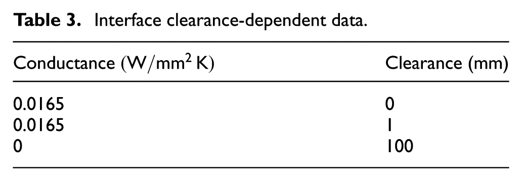
Thermal conductance using clearance-dependent data based on material conductivity (Table 3).

Table 3.

Interface clearance-dependent data.

Conductance $(W / m m^{2} K)$	Clearance (mm)
0.0165	0
0.0165	1
0	100

Analysis procedure

The static analysis type simulated the lateral force acting on the lacing wire. The contact frictional heat, however, is strongly dependent on relative motion.^17,21 The ABAQUS/CAE¹³ solver uses coupled temperature–displacement analysis of simulations involving thermo-mechanical analysis. It takes into account the initial ambient temperature and the relative interaction properties for calculating the transient temperature distribution. Li et al.²¹ carried out a numerical modelling and simulation of friction welding processes based on ABAQUS using coupled temperature–displacement transient. The temperature results were in good agreement with experimentally measured using thermocouples. Correspondingly, this study utilised similar analysis type in simulating the interface frictional thermal generation.

Experimental set-up

The laboratory experimental set-up is presented in Figure 3. Two infrared cameras were used (operated by PC 1). The Micro-epsilon TIM160 infrared camera focused on the friction interface of beam 1. It has a thermal sensitivity of 0.08 K, spectral range of 7.5–13 µm, optical resolution of 160 × 120 pixels, frame rate real time of 120 Hz and lenses’ field of view (FOV) of 23°. On the other hand, Flir A325sc infrared camera focused on the friction interface of beam 2. It has a thermal sensitivity of 0.05 K, spectral range of 7.5–13 µm, optical resolution of 320 × 240 pixels, frame rate real time of 60 Hz and lenses’ FOV of 25°.

Figure 3.

Laboratory experimental set-up.

The Spider box X80 vibration controller (operated by PC 2) first generated the required signals through outputs 1 and 2 for vibration shaker attached to beam 1 (model 4824; Brüel & Kjær) and beam 2 (model MS-1000; Sentek), respectively. The signal for the former was amplified by Brüel & Kjær, model 2732 amplifier while the latter by Sentek, model LA 1500 amplifier. These facilitated the beams’ mechanical excitation. Second, it controlled the vibration excitation via channel 1 by a miniature Deltatron accelerometer type 4507 (sensitivity of 9.989 mV/m/s²) attached to beam 1 for closed-loop operation, thus protecting the shakers against the sudden overloads. Finally, it recorded the friction interface pre-load through channel 4 via a load cell (HBM) with a rated sensitivity of 20 mV/N. The problem of low thermal emissivity of the beams’ surfaces was eliminated by applying black paint which is consistent with standard practice.²² Both beams were excited at 20 Hz, hence facilitated the FEA results’ validation. During the entire excitation period, the thermal images were recorded continuously for 150 s.

Results and discussion

The PC with the 64-bit operating system was used for the simulation. It consisted of four processors each with 3.20 GHz and RAM of 32 GB. The total simulation wall clock time was 272 437 s.

Since the forcing frequencies were periodic, whether the beams are excited in phase or out of phase, the analysed frequencies will be of the same value regardless of the phase. Based on this knowledge, the study considered out-of-phase excitations. The greatest achieved displacement was constant throughout the excitation at 0.10 mm. This was attributed to constant displacement due to periodic loading. Throughout the FEM simulation, two complete cycles of excitation were considered given that the loading was sinusoidal in nature.

When the frictional force moves through a certain distance, a given amount of heat energy is dissipated. The first law of thermodynamics states that at equilibrium, the energy into a system equals the sum of the energy accumulated and the energy output to the environment²³

E_{system} = E_{accumulated} + E_{lost}

(3)

The friction power input is the product of the frictional force F and the sliding speed v. Mabrouki et al.²² reported that frictional energy consumed or stored in the material as micro-structural changes such as dislocations and phase transformation in general is about 5%. The remaining part of the frictional energy raises the interface temperature. Furthermore, Montanini and Freni²⁴ explained that the amount of frictional heat generated depends on several parameters, which include coefficient of friction, normal applied force and the sliding relative speed. However, this study kept other factors constant while the forcing frequencies varied.

Primarily, it is known that frictional heating concentrates within the real area of contact between two bodies in relative motion. In the same breath, according to the Coulomb law of friction, frictional heat generation occurs only if there exists a relative motion between the interacting structures.²⁵ This means that the frictional temperature signature is consistent with the displacement pattern, as evidenced by displacement and frictional temperature time domain waveform for the simulation of both beams excited at 20 Hz (Figure 4) and 40 Hz (Figure 5). As expected, the structure under higher excitation frequency allows the frictional interface to slide against each other more times, unlike at lower frequencies, hence leading to greater frictional temperature evolution as seen with temperature increase from 0.11°C (Figure 6(a)) to 0.20°C (Figure 7(a)) for 20 and 40 Hz, respectively. Moreover, Mabrouki et al.²² observed similar findings on investigation of the frictional heating model for efficient use of vibrothermography. Hence, the conclusion was that frictional heat increases with the interface frequency. The analysed frequencies using a MATLAB Fast Fourier Transform (FFT) algorithm are presented in Figures 6(b) and 7(b). Nevertheless, the observed increasing temperature peak and vice versa for displacement with increasing excitation frequency was attributed to the increasing temperature as explained previously and shortening periodic time considering the same amplitude of displacement, respectively.

Figure 4.

Time domain frictional temperature evolution and displacement (both beams excited at 20 Hz).

Figure 5.

Time domain frictional temperature evolution and displacement (both beams excited at 40 Hz).

Figure 6.

Both beams excited at 20 Hz: (a) interface temperature contour after 0.1 s and (b) FFT of temperature evolution and displacement.

Figure 7.

Both beams excited at 40 Hz: (a) interface temperature contour after 0.05 s and (b) FFT of temperature evolution and displacement.

It was interesting to observe that the frequencies analysed from the frictional temperature evolution were in good agreement with that acquired from the corresponding displacement (Table 4). The relative errors of zero were attributed to periodic loading. However, there existed variation in the spectral peaks among the frequencies predicted by the frictional temperature evolution and the corresponding displacement.

Table 4.

Frequencies for both beams excited at same frequency values.

Forcing frequency for both beams (Hz)	Results	Frequency predicted (Hz)
Forcing frequency for both beams (Hz)	Results	Temp. signature	Disp. curve
20	Figure 6(a)	19.99	19.99
40	Figure 7(b)	39.99	39.99

In the case of beams’ excitation at different forcing frequencies of beam 1 at 20 Hz and beam 2 at 40 Hz, the results revealed a frictional temperature increase of 0.24°C and 0.32°C in the former and latter, respectively (Figure 8(a)). Interestingly, the analysed frictional temperature evolution incredibly predicted the vibration frequency just like displacement curves (Figure 8(b)) as shown in Table 5. Also, the values agreed well with those of the corresponding excitations obtained previously for same excitation frequencies (Table 4). This implies that irrespective of the structural excitations, the analysis of the interface frictional heat evolution is capable enough of predicting its vibration frequency as evidenced by these findings.

Figure 8.

Beam 1 excited at 20 Hz and beam 2 at 40 Hz: (a) interface temperature contour after 0.1 s and (b) FFT of temperature evolution and displacement.

Table 5.

FEA frequencies with different excitation frequencies.

Forcing frequency	Results	Frequency predicted (Hz)
Forcing frequency	Results	Temp. signature	Disp. curve
Beam 1: 20 Hz	Figure 8(b)	19.99	19.99
Beam 2: 40 Hz	Figure 8(b)	39.97	39.97

The crack existence reduces the stiffness of a structural member due to local flexibility. Dimarogonas²⁶ analytically examined the forced vibration of a cracked cantilever beam. The author found that dynamic deflection increases due to crack. This goes a long way to increasing the frictional temperature evolution as shown by the similar contour interface temperature for the healthy model (Figure 9(a)) and vice versa for a model with induced defect (Figure 9(b)).

Figure 9.

Interface temperature contour for both beams excited at 25 Hz after 0.08 s: (a) both beams are healthy and (b) beam 1 induced with defect while beam 2 is healthy.

Even though the frequencies analysed from the frictional temperature signatures and displacements were in good agreement in both models as 25.00 Hz (Figure 10), a significant variation in the peaks existed. Therefore, considering the model with an induced defect in comparison to the healthy model as a reference, the peak for thermally acquired frequency in the case of beam induced with a defect increased and vice versa for the healthy while both increased in the case of displacements. This shows that the presence of structural defect alters the frequency peaks; however, the predominant frequency will be identified based on the spectral peak.

Figure 10.

FFT of temperature evolution and displacement for both healthy and defected FE beam models.

FEM simulation results (Figures 6 and 7) showed that exciting beams at the same value of frequencies and time yield equal maximum frictional temperature. Nonetheless, this was not the case experimentally. The thermal imaging exhibited a temperature difference of 0.9°C (Figure 11) with the ambient temperature being 22.4°C. The frequencies evaluated from the thermal imaging (Figure 11) post analysis of beams 1 and 2 were 19.9885 Hz (Figure 12(a)) and 19.9973 Hz (Figure 12(b)), respectively.

Figure 11.

Thermal images for both beams excited at 20 Hz.

Figure 12.

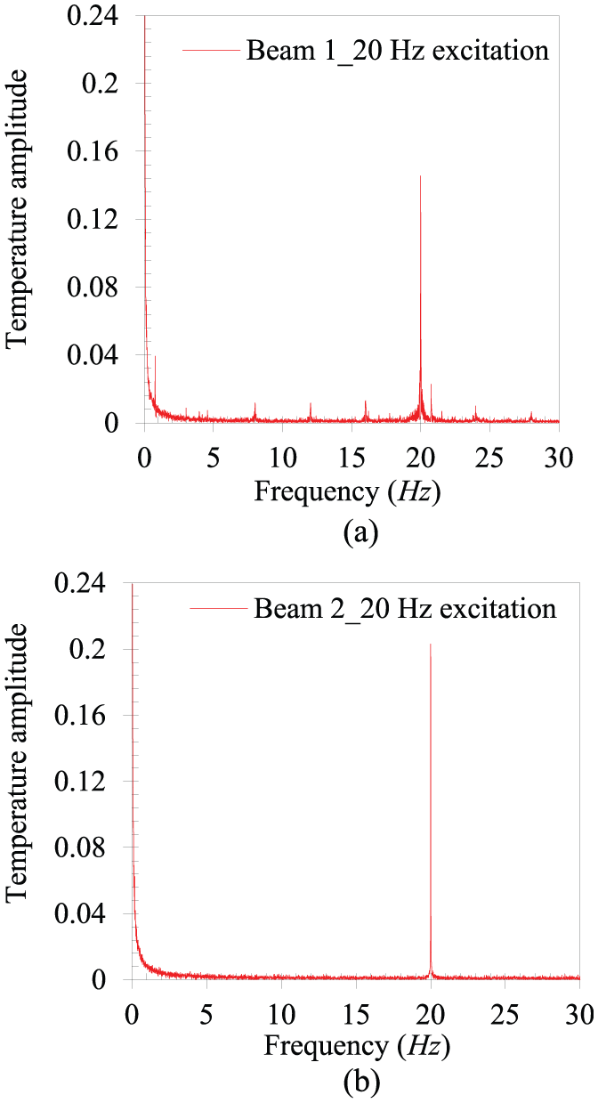
FFT of temperature evolution for both beams excited at 20 Hz: (a) beam 1 and (b) beam 2.

These were in good agreement with the corresponding FEA-predicted frequencies (Figure 6) with relative errors being 0.0075% and 0.0365% for the former and latter, respectively, thus validating the FEM simulation results. Furthermore, beam 1 possessed several smaller frequencies that were associated with the beam multi-dynamics due to periodic loading.

Conclusion

In conclusion, the analysed frictional temperature time domain waveform obtained from the numerical simulation of 3D FEM formulated confirmed the validity in predicting the structural vibration frequency of dynamic mechanical components. Consequently, the presence of a structural defect alters the spectral frequency peaks significantly. Furthermore, the approach developed forms the basis for online monitoring of vibration frequency, hence effective SHM employing IRT. It is important to mention that the finite element modelling and simulation analysis have the ability to perform a detailed mechanical excitation and precise data acquisition at the contact interface that is extremely difficult to be achieved experimentally.

Footnotes

Academic Editor: Crinela Pislaru

Declaration of conflicting interests

The author(s) declared no potential conflicts of interest with respect to the research, authorship, and/or publication of this article.

Funding

The author(s) disclosed receipt of the following financial support for the research, authorship, and/or publication of this article: The authors greatly appreciate the support of Eskom Power Plant Engineering Institute (Republic of South Africa), University of Pretoria and Tshwane University of Technology for funding this research.

References

TTH

Point

Argoul

. Structural changes assessment in axial stressed beams through frequencies variation. Int J Mech Sci 2016; 110: 41–52.

Mukhopadhyay

Chowdhury

Das

. An investigation of the failure of low pressure steam turbine blades. Eng Fail Anal 1998; 5: 181–193.

Rao

SJ.

Turbo-machine blade vibration. 1st ed. New Delhi, India: New Age International Publishers, 1991, pp.7–20.

Safizadeh

Latifi

SK.

Using multi-sensor data fusion for vibration fault diagnosis of rolling element bearings by accelerometer and load cell. Inform Fusion 2014; 18: 1–8.

Al-Bedoor

. Discussion of the available methods for blade vibration measurement. In: ASME 2002 pressure vessels and piping conference, Vancouver, BC, Canada, 5–9 August 2002, vol. 1561, pp.53–61. New York: ASME.

Castellini

Martarelli

Tomasini

EP.

Laser Doppler Vibrometry: development of advanced solutions answering to technology’s needs. Mech Syst Signal Pr 2006; 20: 1265–1285.

Brock

Hayes

Kimbrough

. Dynamic interferometry. In: Proceedings of SPIE 5875, San Diego, CA, 31 July 2005. Bellingham, WA: SPIE.

Sanders

. Turbine steam path engineering for operations and maintenance staff. 1st ed. Canada, ON: Richmond Hill, 1996, pp.236–239.

Straffelini

Friction and wear: methodologies for design and control. Trento: Springer, 2015, pp.21–58.

10.

Bagavathiappan

Lahiri

Saravanan

. Infrared thermography for condition monitoring – a review. Infrared Phys Techn 2013; 60: 35–55.

11.

Kadarno

Taha

Dirgantara

. Vibration analysis of defected ball bearing using finite element model simulation. In: Proceedings of the 9th Asian Pacific industrial engineering and management systems, Nusa Dua, Bali, Indonesia, 3–5 December 2008, pp.2832–2840.

12.

Lie

Cen

Numerical analysis of dynamic behavior of stream turbine blade group. Finite Elem Anal Des 2000; 35: 337–348.

13.

ABAQUS/CAE. Analysis user’s manual. Providence, RI: Dassault Systèmes, 2013.

14.

Petreski

Natural frequencies of a blade group with a lacing wire. Mech Eng Sci 2009; 28: 1–5.

15.

Madhusudana

CV.

Thermal conductance of cylindrical joints. Int J Heat Mass Tran 1999; 42: 1273–1287.

16.

Oden

Martins

JA.

Models and computational methods for dynamic friction phenomena. Comput Method Appl M 1985; 52: 527–634.

17.

Miller

Shih

AJ.

Thermo-mechanical finite element modeling of the friction drilling process. J Manuf Sci E: T ASME 2007; 129: 531–538.

18.

Papuga

Růžička

Meggiolaro

. Computationally-efficient non-linear kinematic models to predict multiaxial stress-strain behavior under variable amplitude loading (3rd international conference on material and component performance under variable amplitude loading (VAL 2015)). Procedia Eng 2015; 101: 285–292.

19.

Claeys

Sinou

Lambelin

. Modal interactions due to friction in the nonlinear vibration response of the ‘Harmony’ test structure: experiments and simulations. J Sound Vib 2016; 376: 131–148.

20.

Arrazola

Özel

Tr.

Investigations on the effects of friction modeling in finite element simulation of machining. Int J Mech Sci 2010; 52: 31–42.

21.

Shi

Wang

. Numerical simulation of friction welding processes based on ABAQUS environment. J Eng Sci Technol Rev 2012; 5: 10–19.

22.

Mabrouki

Thomas

Genest

. Frictional heating model for efficient use of vibrothermography. NDT&E Int 2009; 42: 345–352.

23.

Rajput

RK.

Heat and mass transfer. Ram Nagar, New Delhi: Eurasia Publishing House (P) Ltd, 2006, pp.30–40.

24.

Montanini

Freni

Correlation between vibrational mode shapes and viscoelastic heat generation in vibrothermography. NDT&E Int 2013; 58: 43–48.

25.

Simar

Bréchet

de Meester

. Integrated modeling of friction stir welding of 6xxx series Al alloys – process, microstructure and properties. Prog Mater Sci 2012; 57: 95–187.

26.

Dimarogonas

AD.

Vibration of cracked structures: a state of the art review. Eng Fract Mech 1996; 55: 831–857.

Experimentally validated structural vibration frequencies’ prediction from frictional temperature signatures using numerical simulation: A case of laced cantilever beam-like structures