A method to select correcting faces of a double-face dynamic balancing rotor

Abstract

Considering the sensitivity and installing position limitation, the real positions for two correcting faces must be selected first in the process of double-face dynamic balancing design and practice for rigid rotor system. According to the principle of influence coefficient method, series of testing weight experiments are conducted in this article. Based on the experimental results, the axial distribution laws of the amplitudes and phases of influence coefficients are found and summarized as follows: the amplitude variations of influence coefficients are very small and the phase variations of influence coefficients are obvious when the correcting positions are changed along shaft, so the phases of influence coefficients have the key effect on the correcting vector in correcting faces. Based on this fact, the total phase difference maximum method of influence coefficients is proposed to select the real axial positions for correcting faces. The principle of the method is analyzed in theory, and the application effect is tested by double-face dynamic balancing experiments.

Introduction

Unbalancing vibration has great impact on the working performance, efficiency, and life of the rotor. In order to reduce the unbalancing vibration, suitable dynamic balance technology should be considered during the rotor’s design and application course. In theory, the dynamic balancing method can be divided into two categories: the influence coefficient method and the modal balancing method. Comparatively, the influence coefficient method is an experimental method and its theory is mature. In practical applications, it is unnecessary for operator to spend much time and energy to analyze the structure and build the complex mathematical model for rotor system. Meanwhile, the influence coefficient method is convenient for auto-control and widely applied in rotor dynamic balance.

In practical application, the key questions of influence coefficient method include (1) how to improve the measuring and calculating accuracy of influence coefficient and (2) how to select the real positions of correcting faces.

Recently, many good methods are proposed to improve the measuring and calculating accuracy of influence coefficient.

In 2009, focusing on the problems of small sample and the disturbance of measurement error, an influence coefficient calibration and online updating method was proposed by J Zhang et al. ¹ based on hierarchical Bayesian method for automatic dynamic balancing machine. In 2013, an abnormal value processing method was introduced based on Grubbs criterion to eliminate the influence of gross error by JH Han et al. ² An improved influence coefficient calibration model was proposed, which could solve the system error during the calibration process, and the system error was corrected. In 2013, the 3σ statistical processing method was applied to improve the measuring and calculating accuracy of influence coefficient by AJ Yin et al. ³ In 2012, based on the analysis of rotor dynamics model, the mathematical formula of influence coefficient matrix was discussed by DB Zhu et al., ⁴ who proved the theory that condition number of influence coefficient matrix could measure the accuracy of dynamic balancing. In 2013, based on the complex influence coefficient plant model, YS Liu et al. ⁵ analyzed the tire-rim-spindle dynamics, and a least square based calibration algorithm is developed to calculate influence coefficients. In 2013, the law of phase benchmarks to influence coefficient was studied by GF Bin et al. Based on the phase benchmark, the influence coefficient of the rotor system could be calculated according to the node vibration amplitude and phase of the balancing speed without trial weight. ⁶ In 2013, a scheme was presented by YA Khulief et al., who combined both the influence coefficients and modal balancing techniques. The scheme was developed for low-speed balancing of high-speed rotors and relied on the knowledge of the modal characteristics of the rotor. ⁷ In 2014, in order to solve the non-linear question in influence coefficient method, a new method realized by TS Morais et al. dedicated to the identification of the rotating machinery and the unbalancing distribution in linear and non-linear conditions. The pseudorandom optimization methods and the system modeling were performed using the well-known finite element method. ⁸

In the practical rotor balancing, the theoretical foundation is lacking for selecting the real correcting faces, so the positions of correcting faces are predetermined and inflexible. In this case, the balancing effect is often dependent of discrete parameter, such as pre-defined angular positions and standard balancing weights. ⁹ Because the correcting positions are fixed, the amplitudes of correcting vectors may be too huge to realize when the correcting faces are selected in some insensitive positions.

According to the correcting faces or positions problem, the dimensionless number composed of amplitude difference and phase difference was used to evaluate the quality of influential coefficients in rotor dynamic balancing by PL Han et al., ¹⁰ which proved that the amplitude difference had little effect on the quality of influential coefficients. YT Sun ¹¹ has proved that the amplitude variations of influence coefficients are very tiny when the correcting positions change, but the phase variations of influence coefficients are obvious. ZX Dong et al. ¹² analyzed that the balancing plane positions had a great effect on pathological characteristics of influence coefficient and the interference of dynamic errors could be reduced by selecting locating parameter properly. In 2016, L Li et al. ¹³ discussed the effects of the mass and position of the balancing weight and the rotating speed on the natural frequencies and mode shapes of the blade.

In order to improve the accuracy of influence coefficient and select the real correcting faces for double-face dynamic balance, the total phase difference maximum method is proposed in this article.

The double-face dynamic balancing method

The principle of double-face influence coefficient method

In present, the influence coefficient method is usually applied to calculate the correcting vectors in the course of rotor dynamic balance. The theory and application steps of the double-face influence coefficient are expressed as follows:

• Step 1. The balancing revolving speed should be selected first and then the initial unbalancing vibration signals of monitoring points 1 and 2 on rotor are tested without trial weights. For illustration purposes, the initial unbalancing vibration signals of points 1 and 2 are, respectively, assumed and expressed as $\overrightarrow{V_{0,1}}=V_{0,1}\angle {\phi }_{0,1}$ and $\overrightarrow{V_{0,2}}=V_{0,2}\angle {\phi }_{0,2}$ . (Notes: the symbol “→” expresses the parameter is vector, V is the amplitude of the vector, $\phi$ is the phase of vector, the first number “0” of subscript means without trial weight, the second number of subscript represents the number of monitoring points. The following parameters and symbols have the same meaning unless otherwise noted in this article.)

• Step 2. The trial weight experiments are carried out in correcting face 1. The known correcting vector ( $\overrightarrow{P_1}$ , the number “1” of subscript represents trial weight face) is exerted in correcting face 1 and then the unbalancing vibration signals of monitoring points are measured at the same balancing revolving speed. If the unbalancing vibration vectors of points 1 and 2 are, respectively, assumed as $\overrightarrow{V_{1,1}}=V_{1,1}\angle {\phi }_{1,1}$ and $\overrightarrow{V_{1,2}}=V_{0,2}\angle {\phi }_{0,2}$ (the first number “1” of subscript represents trial weight face), the influence coefficient vectors of the correcting face 1 can be calculated through equation (1)

$$\overrightarrow{R_{1,1}}=\frac{\overrightarrow{V_{1,1}}-\overrightarrow{V_{0,1}}}{\overrightarrow{P_1}},\overrightarrow{R_{1,2}}=\frac{\overrightarrow{V_{1,2}}-\overrightarrow{V_{0,2}}}{\overrightarrow{P_1}}$$

(1)

In equation (1), $\overrightarrow{R_{1,1}}$ are the influence coefficient vectors of the correcting face 1 with respect to monitoring points 1, and $\overrightarrow{R_{1,2}}$ are the influence coefficient vectors of the correcting face 1 with respect to monitoring points 2.

Notes: For easy mathematical operations, all the vectors in equations (1)–(5) are expressed as plural forms. For easy analysis, the amplitudes and phases of the vectors can be calculated from their plural forms.

• Step 3. The similar trial weight experiments are carried out in correcting face 2. If the vector of trial weights is assumed as $\overrightarrow{P_2}$ (the number “2” of subscript represents trial weight face), and the unbalancing vibration vectors of points 1 and 2 are, respectively, assumed as $\overrightarrow{V_{2,1}}=V_{2,1}\angle {\phi }_{2,1}$ and $\overrightarrow{V_{2,2}}=V_{2,2}\angle {\phi }_{2,2}$ (the first number “2” of subscript represents trial weight face), the influence coefficient vectors of the correcting face 2 with respect to points 1 and 2 can be calculated through equation (2)

$$\overrightarrow{R_{2,1}}=\frac{\overrightarrow{V_{2,1}}-\overrightarrow{V_{0,1}}}{\overrightarrow{P_2}},\overrightarrow{R_{2,2}}=\frac{\overrightarrow{V_{2,2}}-\overrightarrow{V_{0,2}}}{\overrightarrow{P_2}}$$

(2)

Notes: $\overrightarrow{R_{2,1}}$ are the influence coefficient vectors of the correcting face 2 with respect to monitoring points 1, and $\overrightarrow{R_{2,2}}$ are the influence coefficient vectors of the correcting face 2 with respect to monitoring points 2.

• Step 4. The correcting vectors of correcting faces can be calculated. Based on the influence coefficients, the correcting vectors of the correcting faces can be calculated by equation (3) if the unbalancing vibration vectors $\overrightarrow{V_{x,1}}$ and $\overrightarrow{V_{x,2}}$ (the symbol “x” denotes the experiment time without trial weight) of points 1 and 2 are tested and taken as the balancing target

$$\left(\begin{array}{cc}\overrightarrow{R_{1,1}}\hfill & \overrightarrow{R_{2,1}}\hfill \\ \multicolumn{1}{c}{\overrightarrow{R_{1,2}}}& \overrightarrow{R_{2,2}}\hfill \end{array}\right)\times \left(\begin{array}{c}\overrightarrow{C_1}\hfill \\ \multicolumn{1}{c}{\overrightarrow{C_2}}\end{array}\right)+\left(\begin{array}{c}\overrightarrow{V_{x,1}}\hfill \\ \multicolumn{1}{c}{\overrightarrow{V_{x,2}}}\end{array}\right)=0$$

(3)

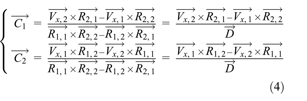
In equation (3), $\overrightarrow{C_1}$ and $\overrightarrow{C_2}$ are assumed as the correcting vectors (the additional unbalancing vectors exerted in correcting faces) of faces 1 and 2. Based on the vector matrix operation method, the vectors of $\overrightarrow{C_1}$ and $\overrightarrow{C_2}$ can be solved and expressed as follows

$$\{\begin{array}{c}\overrightarrow{C_1}=\frac{\overrightarrow{V_{x,2}}\times \overrightarrow{R_{2,1}}-\overrightarrow{V_{x,1}}\times \overrightarrow{R_{2,2}}}{\overrightarrow{R_{1,1}}\times \overrightarrow{R_{2,2}}-\overrightarrow{R_{1,2}}\times \overrightarrow{R_{2,1}}}=\frac{\overrightarrow{V_{x,2}}\times \overrightarrow{R_{2,1}}-\overrightarrow{V_{x,1}}\times \overrightarrow{R_{2,2}}}{\overrightarrow{D}}\hfill \\ \multicolumn{1}{c}{\overrightarrow{C_2}=\frac{\overrightarrow{V_{x,1}}\times \overrightarrow{R_{1,2}}-\overrightarrow{V_{x,2}}\times \overrightarrow{R_{1,1}}}{\overrightarrow{R_{1,1}}\times \overrightarrow{R_{2,2}}-\overrightarrow{R_{1,2}}\times \overrightarrow{R_{2,1}}}=\frac{\overrightarrow{V_{x,1}}\times \overrightarrow{R_{1,2}}-\overrightarrow{V_{x,2}}\times \overrightarrow{R_{1,1}}}{\overrightarrow{D}}}\end{array}$$

(4)

In equation (4), $\overrightarrow{D}$ is an intermediate variable and equal to $\overrightarrow{R_{1,1}}\times \overrightarrow{R_{2,2}}-\overrightarrow{R_{1,2}}\times \overrightarrow{R_{2,1}}$ .

• Step 5. According to the calculating results in equation (4), the corresponding correcting vectors can be exerted in correcting faces and then the unbalancing vibration signals of monitoring points on rotor should be acquired at the balancing revolving speed so as to test the balancing effect.

The above steps indicate that the influence coefficient method is an experimental method, and the balancing effect is greatly affected by the accuracy of influence coefficient. In order to improve the accuracy of influence coefficient, lots of trial weight experiments must be performed, and the means of influence coefficients should be applied to calculate the correcting vectors.

Some discussions on correcting faces

In practical applications, the positions of correcting faces can’t be selected arbitrarily, and the main factors are expressed as follows:

1. From equation (4), the required correcting vectors will be different for the same balancing target when the correcting faces are assembled in different axial positions, and the amplitudes of correcting vectors may be too large to realize in some correcting positions. How to select the sensitive faces with minimum amplitudes of correcting vectors for the same balancing target is a key question which should be resolved in rotor dynamic balancing practice.

2. In equation (3), if there is a minor disturbed error in $\overrightarrow{V_{x,1}}$ and the error is assumed as $\overrightarrow{{\delta }_{x,1}}$ , then the correcting error can be calculated by equation (4) and expressed as equation (5)

$$\{\begin{array}{l}\mathrm{\Delta }\overrightarrow{C_1}=\frac{\overrightarrow{V_{x,2}}\times \overrightarrow{R_{2,1}}-\overrightarrow{V_{x,1}}\times \overrightarrow{R_{2,2}}}{\overrightarrow{D}}-\frac{\overrightarrow{V_{x,2}}\times \overrightarrow{R_{2,1}}-(\overrightarrow{V_{x,1}}+\overrightarrow{{\delta }_{x,1}})\times \overrightarrow{R_{2,2}}}{\overrightarrow{D}}=\frac{\overrightarrow{{\delta }_{x,1}}\times \overrightarrow{R_{2,2}}}{\overrightarrow{D}}\\ \mathrm{\Delta }\overrightarrow{C_2}=\frac{\overrightarrow{V_{x,1}}\times \overrightarrow{R_{1,2}}-\overrightarrow{V_{x,2}}\times \overrightarrow{R_{1,1}}}{\overrightarrow{D}}-\frac{(\overrightarrow{V_{x,1}}+\overrightarrow{{\delta }_{x,1}})\times \overrightarrow{R_{1,2}}-\overrightarrow{V_{x,2}}\times \overrightarrow{R_{1,1}}}{\overrightarrow{D}}=-\frac{\overrightarrow{{\delta }_{x,1}}\times \overrightarrow{R_{1,2}}}{\overrightarrow{D}}\end{array}$$

(5)

In equation (5), $\mathrm{\Delta }\overrightarrow{C_1}$ is the correcting error in face 1, and $\mathrm{\Delta }\overrightarrow{C_2}$ is the correcting error in face 2.

It can be seen from equation (5) that the calculated accuracy of correcting vectors is associated with not only the accuracy of respond signal but also the combined feature of correcting faces. Different combined features can be obtained when the correcting faces are selected in different positions, and the worst combine is when the value of $\overrightarrow{D}$ tends to be zero and the correcting error will be very huge.

• 3. Considering the construction characteristics and assembling requirements of rotor system, the real positions in theory may be limited and other best position should be picked out for correcting faces.

In order to verify and solve the above questions, many dynamic balancing experiments are carried out in this article.

The double-face dynamic balancing experiments and conclusions

In order to research the axial distribution law of influence coefficients, the experimental system is designed and built as in Figure 1.

Figure 1.

The experimental principle of rotor dynamic balance.

In Figure 1, the experimental system is composed of motor system, rotor system, signal acquisition system, and testing weight mechanism. The shaft with multi-diameters and accessories is driven by the motor system through elastic coupling. The eddy current sensors are used to acquire the vibration displacement signals of shaft. In order to calculate the phase of vibration signal, the reference signals must be acquired synchronously. In Figure 1, a wire is twisted into “L” shape and fixed on the shaft, and a photoelectric sensor is used to acquire the position of the wire. A pulse signal will be outputted from the photoelectric sensor when the bending section of wire sweeps the end of photoelectric sensor, and the rising edge of the pulse signal is taken as the zero point of phase. The reference signals can be formed by series of pulse signals during the shaft running, and the phase of vibration signal can be calculated by comparing with the reference signals. The collecting principle of reference signals is shown in Figure 2(a).

Figure 2.

The principle of (a) reference signals acquisition and (b) correcting device.

The signals of sensors are acquired synchronously by acquisition card and analyzed in computer. According to the experimental requirements, the correcting face can be adjusted along the shaft within limits. The device for trial weights and correcting experiment is shown in Figure 2(b).

In Figure 2(b), four same through holes with thread are distributed circumferentially and uniformly along the correcting ring. The correcting ring can be fixed by four same long bolts when the rotor system is running, and the corresponding lock nuts are used to prevent the long bolts from becoming loose. The long bolts and lock nuts can be loosened when the axial position of correcting ring needs to be adjusted. The rubber ring is used to protect the shaft from damage in the process of bolts fastening. Eight same adjusting nuts are divided into four groups and used to adjust and lock the unbalancing vector of each bolt. Based on the vector composition principle, the suitable correcting vector can be gained by adjusting the positions of adjusting nuts. Two similar correcting devices can be taken as the double correcting faces of the rotor system.

Based on the experimental principle in Figures 1 and 2, the real picture of experimental system is shown in Figure 3, and the experimental parameters are listed in Table 1.

Figure 3.

The picture of experimental system.

Table 1.

The experimental parameters.

The diameter of shaft (mm)	50
The length of shaft (mm)	1200
The value of trial weights in face 1 (g mm)	1130
The value of trial weights in face 2 (g mm)	1130
The balancing rotating speed (r/min)	1200

According to the implementation steps of influence coefficient method, serials of double-face trial weight experiments are conducted. In order to mark the axial positions, the geometric center of shaft is selected as the zero point, and the correcting faces can be adjusted symmetrically along both sides of the zero point. Based on the experimental results, the amplitude–position and phase–position curves of influence coefficients are shown, respectively, in Figures 4 and 5.

Figure 4.

The amplitude–position curves of influence coefficients.

Figure 5.

The phase–position curves of influence coefficients.

It can be seen from Figures 4 and 5 that the amplitude variations of influence coefficients are very tiny when the correcting positions are changed, but the phase variations of influence coefficients are obvious, so the conclusion can be drawn that the phases of influence coefficients have the key effect on the correcting vectors of correcting faces. The similar conclusion has been proved by YT Sun. ¹¹

Based on the above influence coefficients, and the initial unbalancing vibration of rotor is taken as the balancing target, the required correcting vectors of correcting faces can be calculated in theory if the two correcting faces are distributed symmetrically on both sides of the shaft, and the amplitude–position curves of correcting vectors are shown in Figure 6.

Figure 6.

The amplitude–position curves of correcting vectors.

The following conclusions can be drawn from Figure 6:

1. When the correcting faces are distributed in different positions, the requiring correcting vectors are different for the same balancing target. In some area, the amplitudes of correcting vectors are too large to realize, and it is called insensitive area for correcting faces, such as the area of [0.2, 0.3] and [−0.3, −0.2]. On the contrary, the amplitudes of correcting vectors are minimum in some area, and the area is called sensitive area for correcting face, such as the area of [0.32, 0.46] and [−0.46, −0.32].

2. When the correcting faces are distributed in some area, the amplitudes of correcting vectors are stable for the same balancing target, and it is called stable area for correcting face, such as the area of [0.32, 0.46] and [−0.46, −0.32].

3. The influence coefficients will be similar when the two correcting faces are distributed to close to each other. The amplitudes of correcting vectors will be huge due to the value of $\overrightarrow{D}$ tending to be zero in equations (4) and (5).

4. The amplitudes of correcting vectors will be huge when the two correcting faces are distributed respectively to close to bearings.

The method for selecting the real correcting faces

Based on the above experiments and conclusions, the correcting face should be selected and designed in the sensitive and stable positions on shaft so as to obtain the good balancing effect. When the best correcting positions can’t be utilized to install the correcting mechanism, other better correcting positions should be selected. For this application requirement, a simple and practical method is introduced as follows.

For illustration purposes, the influence coefficients of correcting faces are expressed as the vector form

$$\overrightarrow{R_{1,1}}=R_{1,1}{e}^{i{\theta }_{1,1}},\overrightarrow{R_{1,2}}=R_{1,2}{e}^{i{\theta }_{1,2}},\overrightarrow{R_{2,1}}=R_{2,1}{e}^{i{\theta }_{2,1}},\overrightarrow{R_{2,2}}=R_{2,2}{e}^{i{\theta }_{2,2}}$$

Notes: R is the amplitude of the influence coefficient vectors, $\theta$ is the phase of the influence coefficient vectors, the first number of subscript denotes the correcting face, and the second number of subscript denotes the monitoring points.

And then equation (4) can be expressed as

$$\{\begin{array}{c}\overrightarrow{C_1}=\frac{\overrightarrow{V_{x,2}}\times \overrightarrow{R_{2,1}}-\overrightarrow{V_{x,1}}\times \overrightarrow{R_{2,2}}}{R_{1,1}\times R_{2,2}{e}^{j({\theta }_{1,1}+{\theta }_{2,2})}-R_{2,1}\times R_{1,2}{e}^{j({\theta }_{2,1}+{\theta }_{1,2})}}\hfill \\ \multicolumn{1}{c}{\overrightarrow{C_2}=\frac{\overrightarrow{V_{x,1}}\times \overrightarrow{R_{1,2}}-\overrightarrow{V_{x,2}}\times \overrightarrow{R_{1,1}}}{R_{1,1}\times R_{2,2}{e}^{j({\theta }_{1,1}+{\theta }_{2,2})}-R_{2,1}\times R_{1,2}{e}^{j({\theta }_{2,1}+{\theta }_{1,2})}}}\end{array}$$

(6)

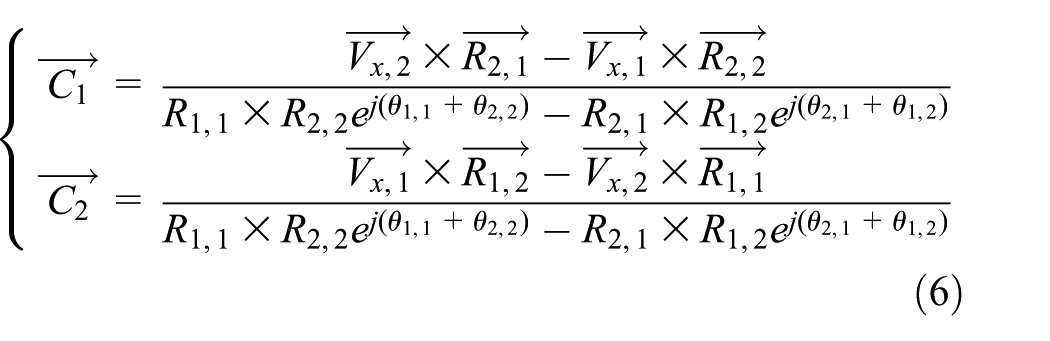
The amplitudes of $\overrightarrow{C_1}$ and $\overrightarrow{C_2}$ can be, respectively, expressed as equations (7) and (8) based on the algorithm of complex number modulus

$$\left|\overrightarrow{C_1}\right|=\frac{|\overrightarrow{V_{x,2}}\times \overrightarrow{R_{2,1}}-\overrightarrow{V_{x,1}}\times \overrightarrow{R_{2,2}}|}{|R_{1,1}\times R_{2,2}{e}^{j({\theta }_{1,1}+{\theta }_{2,2})}-R_{2,1}\times R_{1,2}{e}^{j({\theta }_{2,1}+{\theta }_{1,2})}|}$$

(7)

$$\left|\overrightarrow{C_2}\right|=\frac{|\overrightarrow{V_{x,1}}\times \overrightarrow{R_{1,2}}-\overrightarrow{V_{x,2}}\times \overrightarrow{R_{1,1}}|}{|R_{1,1}\times R_{2,2}{e}^{j({\theta }_{1,1}+{\theta }_{2,2})}-R_{2,1}\times R_{1,2}{e}^{j({\theta }_{2,1}+{\theta }_{1,2})}|}$$

(8)

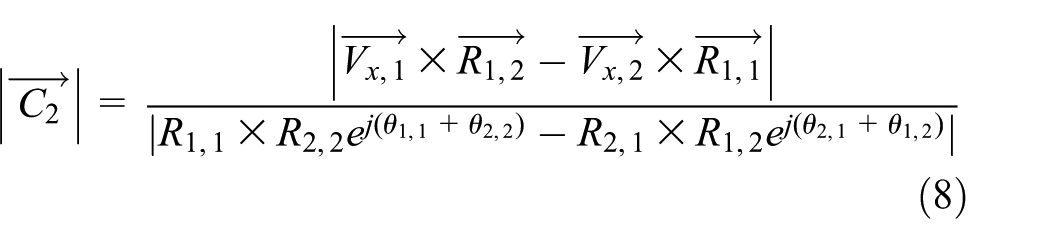
In equations (7) and (8), the amplitudes of influence coefficients can be taken as the constants because their variations are small when the positions of correcting faces are changed along the shaft. In order to reduce the number of variables, three intermediate variables of $\mathrm{\Delta }\theta$ , $\mathrm{\Delta }{\theta }_1$ , and $\mathrm{\Delta }{\theta }_2$ are proposed in this article, and their calculating relations are shown as equation (9)

$$\{\begin{array}{c}\mathrm{\Delta }\theta =({\theta }_{1,1}+{\theta }_{2,2})-({\theta }_{2,1}+{\theta }_{1,2})=({\theta }_{1,1}-{\theta }_{1,2})\hfill \\ \multicolumn{1}{c}{+({\theta }_{2,2}-{\theta }_{2,1})=\mathrm{\Delta }{\theta }_1+\mathrm{\Delta }{\theta }_2}\\ \multicolumn{1}{c}{\mathrm{\Delta }{\theta }_1={\theta }_{1,1}-{\theta }_{1,2}}\\ \multicolumn{1}{c}{\mathrm{\Delta }{\theta }_2={\theta }_{2,2}-{\theta }_{2,1}}\end{array}$$

(9)

In equation (9), the variable $\mathrm{\Delta }{\theta }_1$ is defined as the phase difference between the influence coefficients of correcting face 1. The variable $\mathrm{\Delta }{\theta }_2$ is defined as the phase difference between the influence coefficients of correcting face 2. The variable $\mathrm{\Delta }\theta$ is defined as the total phase difference among the influence coefficients of double-face dynamic balancing system. The variables $\mathrm{\Delta }\theta$ , $\mathrm{\Delta }{\theta }_1$ , and $\mathrm{\Delta }{\theta }_2$ are only associated with the axial positions of correcting faces.

In equation (7), the balancing targets $\overrightarrow{V_{x,1}}$ and $\overrightarrow{V_{x,2}}$ can be taken as constants. If the correcting face 2 is fixed on a constant axial position, the parameters of $\overrightarrow{R_{2,1}}$ , $\overrightarrow{R_{2,2}}$ , and $\mathrm{\Delta }{\theta }_2$ can be taken as constants. Based on the above assumptions, the value of numerator in equation (7) can be taken as constant, and the amplitudes of correcting vectors in correcting face 1 and 2 are determined by the value of denominator. According to the subtraction algorithm of vector, when the amplitudes of operational vectors are constant, the absolute value of phase difference between two operational vectors is nearer to 180°, and the amplitude of composite vector by subtraction operation will be larger. In other words, the value of $\left|\mathrm{\Delta }\theta \right|$ is nearer to 180°, and the amplitudes of correcting vectors will be smaller. Based on this fact, the best correcting face can be selected and this method is defined as the total phase difference maximum method in this article.

In order to test the feasibility of this method, the position of correcting face 2 is set on −0.3 m distance from geometric center of shaft, and the position of correcting face 1 is taken as the variable. Based on the influence coefficients in Figures 4 and 5, the values of $\left|\mathrm{\Delta }\theta \right|$ , $|\overrightarrow{C_1}|$ , and $|\overrightarrow{C_2}|$ can be calculated in theory when the position of correcting face 1 is changed, and their value–position curves are shown in Figure 7.

Figure 7.

The relation between the correcting vector and the position of correcting face 1.

Comparing the curves C11 with C12 and C13 in Figure 7, it can be found that there is an inverse tendency between the amplitudes of correcting vectors and total phase difference. The amplitudes of correcting vectors will be large when the correcting face 1 is distributed in the area of [0.12 m, 0.25 m] and this area is taken as the insensitive area for correcting face 1. The amplitudes of correcting vectors will be unstable when the correcting face 1 is distributed in the area of [0 m, 0.12 m] and this area is taken as the unstable area. The amplitudes of correcting vectors will be small and stable when the correcting face 1 is distributed in the area of [0.32 m, 0.45 m] and this area is taken as the sensitive and stable area. Based on Figure 7, the real positions for correcting face 1 can be selected according to the total phase difference maximum method.

In the same way, the position of correcting face 1 is selected in 0.3 m distance from geometric center of shaft, and the position of correcting face 2 is taken as the variable. Based on the influence coefficients in Figures 4 and 5, the values of $\left|\mathrm{\Delta }\theta \right|$ , $|\overrightarrow{C_1}|$ , and $|\overrightarrow{C_2}|$ can be calculated and their value–position curves are shown in Figure 8.

Figure 8.

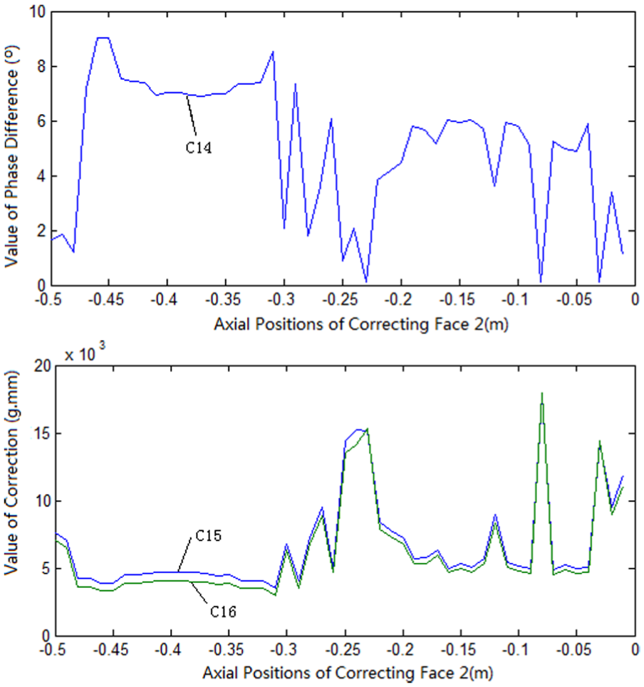
The relation between the correcting vector and the position of correcting face 2.

It can be seen from Figure 8 that the area of [−0.2 m, −0.3 m] can be taken as the insensitive and unstable area for correcting face 2, and the area of [−0.32 m, −0.48 m] can be taken as the sensitive and stable area. The best position of correcting face 2 can be selected based on the total phase difference maximum method.

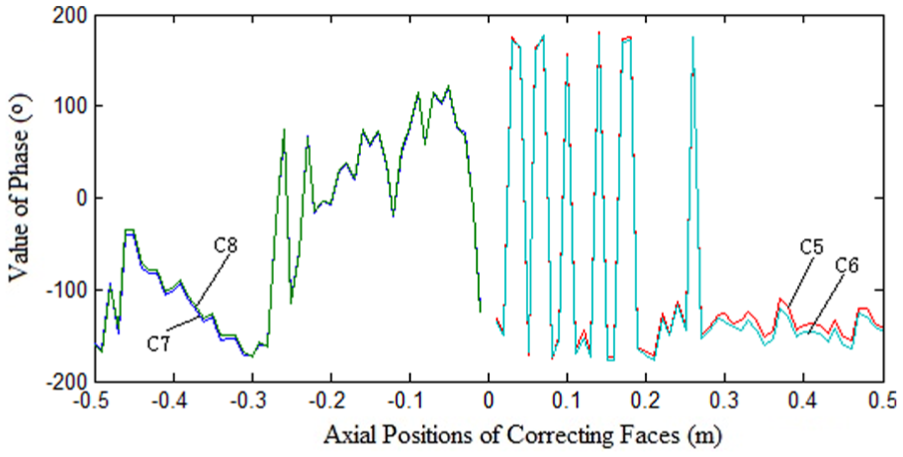
In theory, any unbalance of rigid rotor can be corrected by two correcting faces, ¹³ and the correcting result can be taken as the linear superposition of the correcting effect from two correcting faces. The overall amplitudes of correcting vectors will be minimum when two correcting faces are respectively selected in their sensitive area. So, the total phase difference maximum method can be popularized and applied to select the best correcting faces when all the axial positions of correcting faces 1 and 2 are variable. Based on Figures 7 and 8, the curve of total phase difference can be drawn and shown in Figure 9 when two correcting faces are distributed symmetrically on both sides of the shaft center.

Figure 9.

The phase difference curve of double-face and variable-position balancing system.

Based on Figure 9, the average amplitudes of correcting vectors in correcting faces 1 and 2 on some typical area are calculated and listed in Table 2.

Table 2.

The amplitudes of correcting vectors on some typical area.

Axial positions (m)	[0, ±0.1]	[±0.12, ±0.2]	[±0.22, ±0.32]	[±0.32, ±0.48]
The average amplitudes of correcting vectors in correcting face 1 (g mm)	8383	5700	9050	2456
The average amplitudes of correcting vectors in correcting face 2 (g mm)	8335	5280	8417	1933

It can be seen from Figure 9 and Table 2 that the value of $\left|\mathrm{\Delta }\theta \right|$ is large in the area of [±0.32 m, ±0.48 m], and the amplitudes of correcting vectors will be small when the correcting faces 1 and 2 are symmetrically distributed in this area. So, the best area for correcting faces can be selected in this area.

In practice, if the best area is limited to install the correcting equipment, the second better area of [±0.12 m, ±0.2 m] can be utilized for the correcting faces. On the contrary, the areas of [0 m, ±0.1 m] and [±0.22 m, ±0.32 m] shouldn’t be selected as the correcting faces because the amplitudes of correcting vectors are very large.

If the positions of correcting faces can be selected arbitrarily on shaft, the best correcting positions of faces 1 and 2 can be selected, respectively, from Figures 7 and 8 based on the total phase difference maximum method. For example, if the correcting position of face 1 is selected in the position of 0.34 m from Figure 7, and the correcting position of face 2 is selected in the position of 0.45 m from Figure 8, then the amplitudes of correcting vectors in faces 1 and 2 can be calculated as 2192 and 1717 g mm.

It can be seen from the above discussions that the total phase difference maximum method is built on the testing weight experiments and the calculation of influence coefficient. For practical application, the performing steps are summarized as follows:

• Step 1. The vibration monitoring points and some special correcting positions are selected first. After that, according to the principle influence coefficient method, series of trial weight experiments are performed and the influence coefficients of each correcting positions are calculated. After all the trial weight experiments are completed, the phase differences of each correcting positions should be calculated based on their influence coefficients and then the curve of total phase difference can be drawn.

• Step 2. The real correcting positions can be selected based on the rotor structure and the total phase difference curve. For easy selection, the correcting positions can be divided into two parts based on the geometric center of shaft, and the left and right areas can be taken, respectively, as the alternative positions of correcting faces 1 and 2. According to the values of the total phase differences, the sensitive and stable areas in the left and right parts of shaft can be selected respectively for correcting faces.

• Step 3. The superiority and balancing effect of real correcting positions are tested through theoretical calculation and experimental analysis. Several typical positions can be chosen to calculate the correcting vectors according to equations (7) and (8) and then the superiority of the real correcting positions can be confirmed in theory. According to the calculating results, the suitable correcting vectors can be exerted in corresponding correcting faces and then the unbalancing vibration signals of monitoring points are tested. The balancing effect can be tested by comparing the current amplitude with initial amplitude of unbalancing vibration signals.

Conclusion

1. Many experiments have proved that the sensitive and insensitive correcting faces exist in rotor dynamic balance. The amplitudes of required correcting vectors will be too big to realize when the correcting faces are designed in insensitive positions. On the contrary, the good balancing effect can be gained even if the amplitudes of correcting vectors are minor in sensitive positions. Meanwhile, limited by structure characteristics and accessory installation of rotor system, some positions in shaft can’t be used to install the dynamic balance mechanism. So, it is a key question to select the real correcting faces for multi-face rotor dynamic balance.

2. The testing weight experiments indicate that the amplitude variations of influence coefficients are very small and the phase variations of influence coefficients are obvious when the correcting face position is changed along shaft. The phase of influence coefficients has the key effect on the correcting vectors of correcting face. Based on this fact, the total phase difference maximum method of influence coefficients is proposed to select the best correcting positions for multi-face dynamic balancing system. The application effect of the method is proved by dynamic balancing experiments.

3. According to the derivation process of the total phase difference maximum method of influence coefficients, it can be popularized and applied to select the real correcting faces for multi-face dynamic balance of flexible rotors, and it has the similar application steps.

First, the influence coefficients of finite positions are tested and calculated by trial weight experiments in the selectable region of each correcting face.

Second, the position of one correcting face is assumed to be variable, and the positions of other correcting faces are assumed to be fixed. Based on the total phase difference maximum method of influence coefficients, the sensitive position of this correcting face can be selected. According to this method, the sensitive positions of other correcting faces can be selected in the same way.

Third, based on the principle of linear superposition, the correcting effect of every correcting face corresponding to the same monitoring point is independent of each other, so the selected sensitive positions in second step can be taken as the real correcting faces for multi-face dynamic balance of flexible rotors. And then the superiority and balancing effect of these real correcting positions are tested through theoretical calculation and experimental analysis.