Sage Journals: Discover world-class research

Abstract

Nonlinear behavior is often observed in structural joint system due to external loads. A new technique of nonlinear structural joint model updating with static load test results is proposed in this article to investigate the actual behavior of a joint system. To calibrate the nonlinear parameters of the structural joint system, an appropriate finite element model is first established to characterize the complex nonlinear behavior caused by the joint connections. Combined with the sensitivity analysis, the parameters that describe the nonlinear behavior of the joint connections are selected as the parameters to be updated. Subsequently, an objective function is created in accordance with the residual between experimentally measured static deflections and analytically calculated static deflections through finite element model. The objective function is then optimized to obtain the proper values of the nonlinear force–displacement parameters with the regular simulated annealing algorithm. To validate the efficiency of this updating approach, two numerical examples under static concentrated loads are conducted. The obtained results indicate that the nonlinear joint model parameters can be successfully updated, and the updated new model can further forecast the true deflections of the nonlinear structure with good accuracy and stability.

Keywords

Nonlinear joint model updating sensitivity analysis simulated annealing nonlinear force–displacement relationship static deflection

Introduction

Joint connections exist widely in many large-scale complex structures. Static and dynamic responses of these structures are significantly affected by the joints due to their complicated and nonlinear properties. Traditional linear model and straight-forward joint coupling will no longer be applicable to this system. Therefore, in order to achieve a more precise expression of the structural behavior, it is essential to consider these additional joint effects and find a more proper method to model and update the joints.

Driven by the advances in sensor technology and computational power, modeling and updating the nonlinear behavior of joints has undergone a dramatic development in recent decades. Multiple issues have been published in this regard. For instance, special attention was given to the modeling of welded joints by Ahmadian et al.¹ Mackerle² presented a detailed review on various types of joints for finite element analysis from both theoretical and practical points of view. Ahmadian et al.³ modeled the joint with a thin-layer interface element and updated the model via a sensitivity method in the AWE-MACE system. Dias et al.⁴ presented a three-dimensional (3D) nonlinear model to study the structural behavior of timber–concrete joints. Using special contact elements, such as thin-layer and zero thickness elements, Mayer and Gaul⁵ proposed an effective method to simulate the contact interfaces of joint connections. Bograd et al.⁶ presented a comprehensive review of various methods for dynamic model establishment of structural joints in assembled structures. It generally includes the contents about joint features, types of joint connection, and brief simulation models of joint for the assembled structures.

Many researchers have also investigated the nonlinear behavior of joints. For example, Gaul and Lenz⁷ investigated the joint effects on the nonlinear dynamic behavior through both experimental and numerical studies. In that study, they proposed an improved lumped parameter model and identified the parameter with experimental research. Girão Coelho et al.⁸ described an appropriate finite element model to characterize the complex performance of the bolted connections. The joint interface is simulated by node-to-node contact elements. Schwingshackl et al.⁹ further studied the modeling approach of the bolted flange joints. To correctly characterize the nonlinear dynamic behavior, they developed an advanced modeling technique which brought on an excellent agreement with the experimental data. By introducing layered method and constitutive law, Khorsandnia et al.¹⁰ conducted the nonlinear finite element model analysis of timber, timber–concrete composite beams and joints.

In the application of parameters identification and updating of joints, Yang et al.¹¹ developed a matrix formula for joint model and proposed a parameter identification approach for joints through substructure synthesis technique and frequency response function. Cunha et al.¹² successfully identified the stiffness of joints in a frame structure by conducting a model updating approach with both static and dynamic responses. With single-frequency excitations, Jalali et al.¹³ obtained the parameters of the bolted joint model by force-state mapping of acceleration responses in time domain. Combined with empirical mode decomposition, Eriten et al.¹⁴ performed the nonlinear system parameter identification for the friction joint connections in a bolt assembled beam. Mehrpouya et al.¹⁵ investigated the inverse receptance coupling approach and the point-mass model and further identified the joint dynamic properties using frequency response functions.

Iranzad and Ahmadian¹⁶ simulated a bolted joint by a thin layer with elastic–plastic material and conducted the nonlinear model updating procedure to identify the material parameters with measured results. In their article, thin-layer material properties are regarded as design variables and the difference between measured and model predicted frequency response functions is used for objective function. By minimizing the objective function, proper values of design variables are found and model parameters are identified. Alamdari et al.¹⁷ adopted the Richard–Abbot elastic–plastic material to characterize the nonlinear stress–strain relation of joint interface element. Then, the four material parameters were updated by minimizing the residual between measured and analytical nonlinear frequency response functions with iterative sensitivity-based optimization algorithm. Using a two-step Kalman filter approach and partial measurements of structural acceleration responses, Lei et al.¹⁸ proposed a novel algorithm for damage detection of frame structures suffering joint damage from earthquake excitation. Davoodi et al.¹⁹ introduced a general nonlinear relationship of joint connections and considered the curve coefficients as the parameters to be updated. With genetic algorithm and static deflections, they determined the nonlinear static performance of the ball joint system by model updating technique.

This study focuses on developing a physically meaningful model to characterize the complex nonlinear behavior of the joint system under static loads. Accordingly, an innovative nonlinear structural model updating method based on static load test results is proposed to research the true performance of joint system. First, a proper finite element model is introduced to describe the nonlinear behavior of the joints. Combined with sensitivity analysis, the parameters that describe the nonlinear force–displacement curve of the joints are selected as the parameters to be updated. Then, an objective function is created on the basis of the residual between experimental static deflections and analytical static deflections calculated by the simulated finite element model. After that, with a well-known simulated annealing (SA) algorithm, the optimization problem is solved to obtain the proper values of the nonlinear force–displacement parameters. Finally, a more reasonable model can be obtained to describe the actual behavior of the joint system under both the load used for updating and the new load.

The organization of this article includes the following parts: first, an overview of the modeling and updating for joints is presented. Next, a detailed description of a nonlinear joint model updating technique is provided, followed by a characterization of a nonlinear force–displacement relationship model that has been used in this study. Then, two simulated numerical examples are performed for validating the effectiveness of this presented approach. Finally, the article ends with conclusions and lists some recommendations for future work.

Theoretical background

Nonlinear joint model

To study the joint effects on a structural system, an appropriate element should be selected to simulate the joints. In this article, a one-dimensional (1D) spring element (Combin39, which is from software ANSYS²⁰) with generalized nonlinear force–displacement capability is introduced to model the joint connections for nonlinear finite element model analysis. This element can be applied to simulate the longitudinal force–displacement or torsional moment–rotation relationship in 1D to 3D systems.

As shown in Figure 1, the nonlinear force–displacement curve of Combin39 element can be defined by sequentially connecting a series of points. These points on the graph (D1, F1, etc.) denote forces (or moments) against relative translations (or rotations) in the structural analysis. It is noteworthy that the nonlinear force–displacement relationship parameters should be input in sequence to make sure that the displacements increase from the third quadrant (compression region) to the first quadrant (tension region) of the coordinate system. The fundamental aim of this article is to determine the coordinates of these points using nonlinear joint model updating technology. The force coordinates of these points are fixed in advance according to the approximated force range and the displacement coordinates are considered as parameters to be determined after model updating. Considering the restriction in ANSYS software, computational accuracy, and time consumption, a total of 19 points have been utilized to depict the nonlinear force–displacement relationship curve of Combin39 element. Specifically, these 19 points are composed of 9 points in compressive zone, 9 points in tensile zone, and 1 origin point.

Figure 1.

Nonlinear force–displacement curve for Combin39.

Sensitivity analysis

The sensitivity analysis is usually conducted in order to select the most important variables for the finite element model updating program. Many researchers have also applied sensitivity analysis to inelastic structures, nonlinear mechanics, and earthquake engineering.^21–23 The sensitivity coefficient S is generally defined as the ratio of the change in a specific response quantity (such as natural frequency) and the change in a variable (such as elastic modulus). The sensitivity coefficients about the relevant parameters can be calculated with direct derivation or perturbation methods.²⁴ As for this study, the sensitivity coefficients are approximately calculated by centered difference technique, which is a computationally efficient and accurate approach for computing the response sensitivity. Since the sensitivity calculation involves different kinds of parameters (such as axial, bending stiffness), the sensitivity coefficient is normalized in this article. The normalized relative sensitivity coefficient is defined as

S_{ij} = \frac{δ λ_{i}}{δ x_{j}} \frac{x_{j}}{λ_{i}} \approx \frac{λ_{i} (x_{j} + Δ x_{j}) - λ_{i} (x_{j} - Δ x_{j})}{2 Δ x_{j}} \frac{x_{j}}{λ_{i} (x_{j})}

(1)

where $S_{ij}$ is the normalized relative sensitivity coefficient of response $λ_{i}$ in respect of parameter $x_{j}$ , and $Δ x_{j}$ is the considered perturbation in the parameter, taken to be 0.01 $x_{j}$ in this study.

Considering the truth that static deflection of a structure is among the most important responses that can reflect the accuracy of the analysis, in this article, $λ_{i}$ is suitably defined as vertical deflection of selected node i obtained by the analysis using ANSYS finite element analysis software and $x_{j}$ is the jth parameter variable which may be used later for model updating.

Objective function

The objective function $Π$ can be defined to indicate the residual between the measured responses and corresponding analytical responses for a structure. Then, the nonlinear model updating program is turned into an optimization problem so as to seek $x^{*}$ that satisfies

Π (x^{*}) \leq Π (x), x_{li} \leq x_{i} \leq x_{ui}

(2)

in which the minimum and maximum values of the parameters should be given in advance, guaranteeing the physical significance of the parameter values.²⁴

In this study, an objective function form that consists of the residual between measured static deflections and corresponding static deflections gained through numerical model analysis is introduced to carry out the nonlinear model updating problem for the joint system. Taking the structural nonlinear load–deflection behavior into account, the numerical static deflections are compared with the measured static deflections at several different load steps. Thus, the objective function is formulated as follows

J (θ) = \frac{1}{N_{1} \times K_{1}} \sum_{i = 1}^{n_{1}} {\sum_{j = 1}^{k_{1}} (\frac{d_{i}^{j} - d_{i}^{j} (θ)}{d_{i}^{j} (θ)})}^{2}

(3)

where $d_{i}^{j}$ is the experimental static deflection of node i at load step j and $d_{i}^{j} (θ)$ is the corresponding numerical deflection of node i at load step j, and $θ$ is the vector of the parameters to be updated. $N_{1}$ and $K_{1}$ are the number of selected nodes and the number of load steps, respectively. Therefore, the objective function consists of $N_{1} \times K_{1}$ parts, with each part being square of the relative percent error between the measured and numerical static deflections for node i at load step j. Steps of load are uniformly distributed and increased until the peak load is applied to the structure.

The updated results are then evaluated by two proposed error indices that are deflection errors between real model and updated model. These error indices are defined as follows

E_{1} = \sqrt{\frac{1}{N_{2} \times K_{2}} {\sum_{i = 1}^{n_{2}} \sum_{j = 1}^{k_{2}} (\frac{d_{i r e a l}^{j} - d_{i d a t e d}^{j}}{d_{i r e a l}^{j}})}^{2}} \times 100 %

(4)

E_{2} = \max {\frac{| | d_{i r e a l} - d_{i d a t e d} | |_{2}}{| | d_{i r e a l} | |_{2}}} \times 100 %

(5)

where $d_{i real}^{j}$ and $d_{i updated}^{j}$ are real and updated static deflections of node i at load step j, respectively. $N_{2}$ and $K_{2}$ are the number of nodes and the number of load steps, respectively. $d_{i real}$ and $d_{i updated}$ are the real and updated static deflection vectors of node i, respectively. $| | \dots | |_{2}$ represents two-norm value.

Optimization technique

Using indirect methods, the nonlinear joint model updating procedure is implemented by solving an optimization problem with the target to minimize the objective function under specific constraints. A series of method accessible for solving the constrained optimization problem (such as genetic algorithm, artificial neural network, and harmony search algorithm)^25–27 have been proposed in the past decades. In this study, the optimization problem of nonlinear joint model updating is considered as a constrained minimum problem that consists of many optimization variables and a relatively complex objective function. Thus, the commonly used SA algorithm²⁸ is introduced to solve this issue.

SA, which is a probabilistic search algorithm to seek the global minimal value among large amounts of local minima, has been widely used in civil engineering for the model updating.^29,30 Some researchers have also proposed modifications to the standard SA to accelerate the convergence. For instance, Ingber³¹ developed a very fast simulated re-annealing algorithm. Levin and Lieven³² studied dynamic finite element model updating with SA and genetic algorithms. Jeong and Lee³³ presented an efficient adaptive SA genetic algorithm for system identification. Combining SA with the unscented Kalman filter, Astroza et al.³⁴ proposed a new method for finite element model updating. As an extension of local search algorithm, SA algorithm generates a new state model in every modified process and selects the state containing largest energy value with a certain probability. This new acceptance criterion makes SA be a global optimization algorithm. Furthermore, as an effective nonlinear optimization algorithm, SA has been proved to be strict in theory and effective in practice.

Since the deflection responses in the objective function are obtained numerically by finite element analysis software, the SA optimization algorithm is incorporated with ANSYS to solve the multi-variables constrained optimization problem. A MATLAB-based optimization procedure³⁵ has been proposed for this study. The overall stages of the nonlinear joint model updating process are shown in Figure 2. Therefore, to perform the nonlinear joint model updating program, different steps involved in the process, as depicted in Figure 2, are executed sequentially using the prepared program as follows:

Initialization and annealing plan: first, the parameters involved in the optimization technique are initialized. Then, to simulate the annealing process, the annealing plan is conducted as $T_{k} = T_{0} \exp (- λ (k - 1)^{γ})$ for the kth outer cycle, where $T_{k}$ is the current temperature, $T_{0}$ is the initial temperature, $λ$ and $γ$ are attenuation coefficients, and k is iteration number.

Model disturbance: in this inner cycle, parameters to be modified are disturbed as $θ_{k} = A + δ_{k} \cdot (B - A)$ , where A and B are the minimum and maximum values of the variables, respectively, $δ_{k}$ is a vector with each element randomly distributed between 0 and 1.

Acceptance criteria: based on the objective function values and Metropolis rule, the model acceptance criterion is defined as follows: (a) if $Δ J < 0$ , the new parameters are accepted; (b) if $Δ J \geq 0$ , a variable $ξ$ is produced randomly between 0 and 1, then if $\exp (- Δ J / T_{k}) > ξ$ , the new parameters are also received, else they will be discarded.

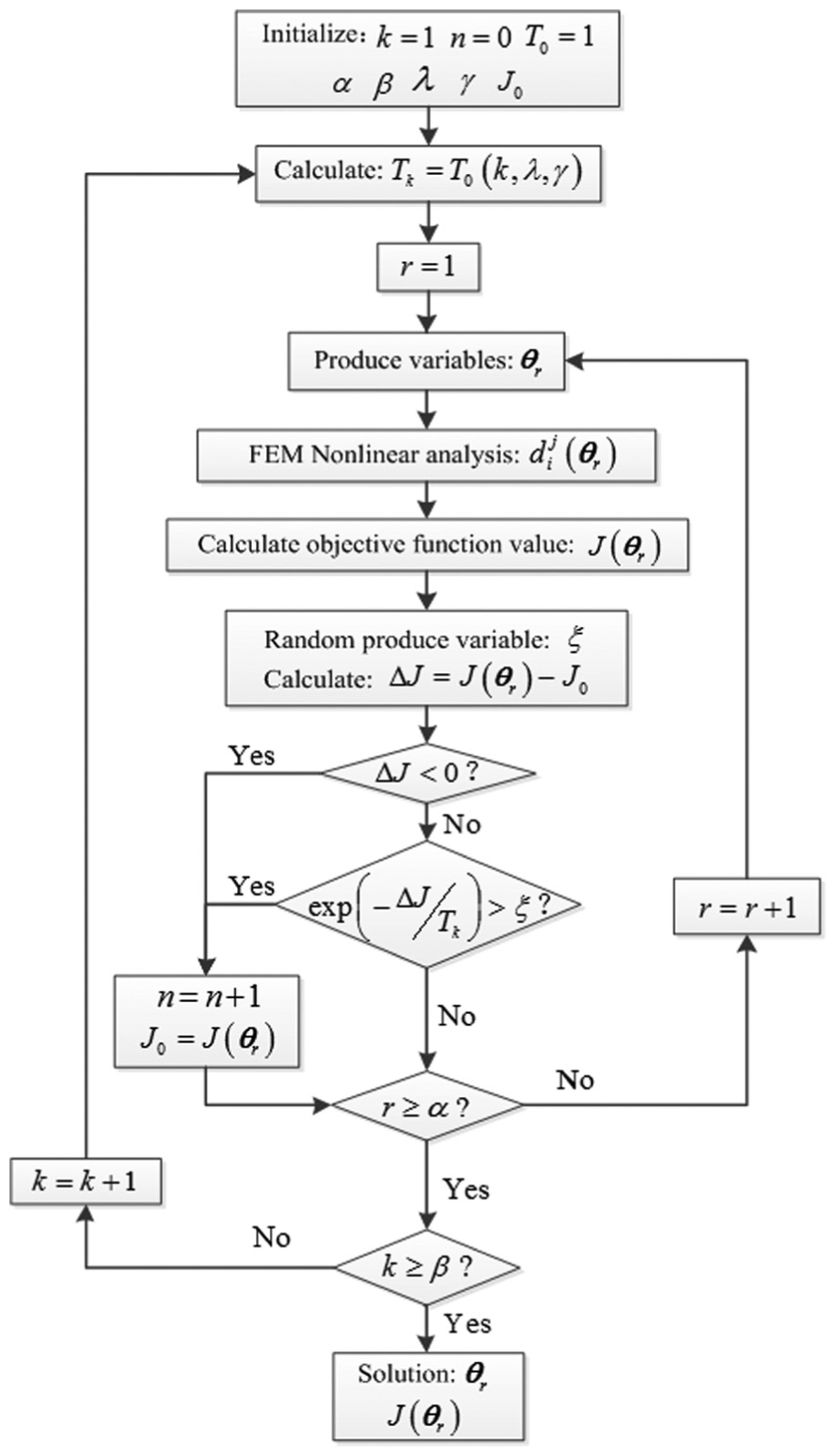
Termination: for each inner cycle, the procedure stops and turns to the next inner cycle when the inner number r reaches $α$ , and the procedure stops finally when the outer number k reaches $β$ . As a result, the last accepted parameters that have the minimum objective function value are thought of as the optimal estimation of updated parameters.

Figure 2.

Overall steps of the nonlinear joint model updating technique using SA.

Numerical verification

Simulated cantilever beam with nonlinear joint supports

In this section, a simulated cantilever beam with nonlinear joint supports is aimed at demonstrating the efficiency of the nonlinear joint model updating technique mentioned above. The main task in this case is to update the nonlinear force–displacement curve parameters so that the analytical responses provide a good agreement with measured results of the beam. Static deflections are obtained through finite element analysis to construct an objective function as shown in equation (3). Using SA algorithm, the force–displacement parameters on behavior of the nonlinear properties of the structure are then updated with the minimum objective function value.

Model description

In this case, the finite element software ANSYS is applied to analyze this beam. As illustrated in Figure 3, the cantilever beam with nonlinear joint supports is first modeled. Beam3 element (which is an elastic uniaxial element with tension, compression, and bending capabilities) is used to simulate the beams, while Combin39 element is introduced for simulating the nonlinear relationship of the joint supports. The translation in the nodal x-direction of Beam3 element has been fixed. The length of each Beam3 element is 50 mm. The beam section is rectangle whose width and thickness are 20 mm and 15 mm, respectively. Its material properties are as follows: elastic modulus E = 210 kN/mm² and Poisson ratio v = 0.3.

Figure 3.

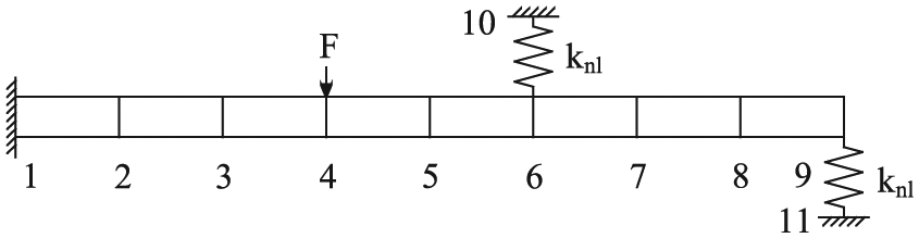
Detail description of the beam.

The whole finite element model consists of 8 beam elements, 2 nonlinear spring elements, and 11 nodes. It is assumed that the two spring elements share the same force–displacement relationship. Static concentrated load (F = 5.5 kN) is divided into 10 steps and applied to node 4 step by step.

Nonlinear joint model updating

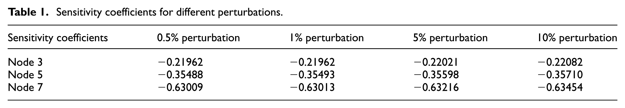
As mentioned previously, the sensitivity analysis is first done. The $x_{j}$ in equation (1) is considered to be the initial stiffness of the nonlinear spring, which is set to be 0.32 kN/mm. Then, the sensitivity analysis is conducted for different perturbations (0.5%–10% perturbations) and the obtained normalized relative sensitivity coefficients corresponding to the deflections of nodes 3, 5, and 7 are listed in Table 1. It can be known that the sensitivity coefficient changes only a little with the increment of perturbation. Therefore, combined with some previous references, 1% perturbation is adopted in this article. The deflections of nodes 3, 5, and 7 reduce about 0.22%–0.63% with respect to 1% increment in the stiffness. This indicates the high sensitivity of node deflection to the spring stiffness. Therefore, the stiffness of joint supports is simulated with Combin39 element for nonlinear joint model updating.

Table 1.

Sensitivity coefficients for different perturbations.

Sensitivity coefficients	0.5% perturbation	1% perturbation	5% perturbation	10% perturbation
Node 3	−0.21962	−0.21962	−0.22021	−0.22082
Node 5	−0.35488	−0.35493	−0.35598	−0.35710
Node 7	−0.63009	−0.63013	−0.63216	−0.63454

The nonlinear joint model updating process is to correlate the nonlinear force–displacement curve parameters to match the measured static deflections. In this case, the force coordinates of these nonlinear force–displacement curve points are uniformly increased from −0.72 to 0.72 kN according to the approximated force range. Then, the updating parameters vector is defined as $θ = {θ_{1}, θ_{2}, \dots, θ_{18}}$ with 18 representing the number of points to be updated in the nonlinear force–displacement curve. The parameters θ₁–θ₉ reflect the nonlinear characteristic of joint supports in the compressive region, while the parameters θ₁₀–θ₁₈ correspond to that in the tension zone. The parameters $θ_{exact}$ (listed in Table 2) are used to calculate the static responses as measured responses. It is very hard to estimate the variation bound. In fact, it can be assumed according to some engineering judgment. In the studies of Zhang et al.,^36,37 the maximum variation of ±40% is given for some uncertain parameters. In order to guarantee the physical significance, the parameters $θ$ to be updated are restricted between 0.7 and 1.3 times of the parameters $θ_{exact}$ . Then, following the stages in Figure 2, the nonlinear joint model updating program is conducted to obtain the optimal values $θ_{updated}$ that makes the objective function defined in equation (3) minimum.

Table 2.

Updated parameters and values of objective function.

Runs	Parameters of the nonlinear force–displacement relationship θ₁–θ₁₈									$J (θ) (\times 10^{- 4})$
Exact (measured)	−2.89	−2.46	−2.07	−1.71	−1.38	−1.07	−0.78	−0.51	−0.25	/
Exact (measured)	0.25	0.51	0.78	1.07	1.38	1.71	2.07	2.46	2.89	/
Updated (the first run)	−2.85	−2.42	−2.10	−1.68	−1.37	−1.09	−0.77	−0.49	−0.23	1.154
Updated (the first run)	0.31	0.56	0.79	1.10	1.38	1.72	2.06	2.34	2.76	1.154
Updated (the second run)	−2.94	−2.53	−2.09	−1.69	−1.39	−1.10	−0.83	−0.55	−0.29	2.031
Updated (the second run)	0.20	0.46	0.69	0.98	1.24	1.62	2.06	2.37	2.86	2.031

The objective function can be created using the deflections of a series of nodes and a reasonable estimated result can be obtained. In order to discuss the effects of selected node number, total four cases are considered in this study. Case 1: Eight nodes are uniformly selected along the structure as measuring points and the deflections of these points are used for updating. Case 2: Four nodes are uniformly selected along the structure as measuring points and the deflections of these points are used for updating. Case 3: Two nodes are uniformly selected along the structure as measuring points and the deflections of these points are used for updating. Case 4: One node is uniformly selected along the structure as measuring point, and the deflection of this point is used for updating.

In order to obtain acceptable accuracy with low computation cost, the values of the variables involved in the SA algorithm are carefully selected. These are as follows: $T_{0}$ , $λ$ , $γ$ , $α$ , and $β$ are 100, 0.5, 0.6, 10, and 300, respectively. Considering the stochastic generation of the initial parameters $θ$ in the SA algorithm, the nonlinear joint model updating process has been run 20 times for each case. Figure 4 shows the representative record of improvement in the objective function value for Case 3. It can be known that the value decreases rapidly during the first few iterations and reaches to a nearly constant value after about 95 iterations. It indicates that the convergence speed is acceptable. Due to the stochastic generation of the initial parameters in the SA algorithm and the number of equilibrium iterations in the nonlinear static analysis, the required time for completing the updating process varies between 19 and 32.5 min on a 3.2 GHz PC. Most of this time is spent by nonlinear static analyses of the structure. Only a little time is spent on the optimization.

Figure 4.

The function values with progression of iterations for cantilever beam.

The deflections of all the eight nodes are introduced for equations (4) and (5) to evaluate the accuracy of updated model. The statistical properties of the error indices (mean µ and standard deviation σ of the 20 runs) for these four cases are shown in Figure 5. It can be seen that with the decrease in the selected point number, the defined error indices show an increasing tendency. However, this increasing trend is not significantly obvious when two or more nodes are selected. The error indices of Case 4 are much bigger than that of other cases. Therefore, in order to obtain higher accuracy with fewer measuring points, Case 3 is introduced for the nonlinear joint model updating in this study.

Figure 5.

The error indices for the four cases.

Figure 6 shows the nonlinear force–displacement relationship curves of the joint supports achieved through nonlinear joint model updating (2 runs of the 20 runs). Each figure includes the exact force–displacement relationship (which is defined to calculate static responses as measured responses), initial force–displacement relationship, and the force–displacement relationship obtained via conducting the updating process once. According to these figures, it can be known that for all the two runs, the updated parameters $θ_{updated}$ match well with the exact parameters $θ_{exact}$ except individual points in the force–displacement curve. The updated 18 parameters of nonlinear force–displacement relationship and the corresponding values of the objective function for all the two runs are presented in Table 2. It can be observed that the nonlinear joint model parameters can be availably updated with high accuracy and stability using the presented model updating method.

Figure 6.

Comparisons of nonlinear force–displacement relationship curves between exact and updated results for cantilever beam: (a) the first run and (b) the second run.

After updating, the updated new model with obtained parameters is analyzed. The load–deflection curves of the three nodes acquired by the analysis of both exact and updated nonlinear finite element models are shown in Figure 7. It can be seen that there exists an excellent matching between the updated and exact (measured) load–deflection curves for all these nodes. Therefore, the nonlinear force–displacement relationship obtained by the proposed model updating technique can reflect the true behavior of the joint system.

Figure 7.

Comparisons of nonlinear load–deflection relationship curves of nodes 3/4/6 between exact and updated results: (a) the first run and (b) the second run.

In order to verify the validity and accuracy of this updated nonlinear joint model under other loads, another different concentrated load (F = 4.5 kN) is then applied to node 5. Then, the exact, initial, and updated models are analyzed. The load–deflection curves are compared in Figure 8. As one can see from Figure 8, the updated new nonlinear joint model can correctly predict the responses subjected to other loads.

Figure 8.

Comparisons of nonlinear load–deflection relationship curves of nodes 3/4/6 between exact and updated results (under the new load): (a) the first run and (b) the second run.

Noise effects

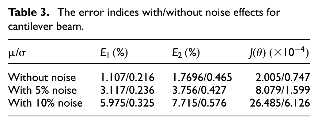
To further study the noise effect, the simulated deflections with 5% and 10% noise are, respectively, assumed as the measured responses for every load step. In the case of 5% noise, the noise is randomly generated between −5% and +5% of the deflection amplitude. For larger level of noise, the same approach is used to add 10% noise into the simulated deflections. The original and noise contaminated deflections at the last load step are presented in Figure 9. Again, the updating program has been run. The accuracy of updated nonlinear model is also evaluated using the defined error indices and the results are presented in Table 3. As one can see from Table 3, the proposed method can obtain the nonlinear model parameters even with noise effect. For the case with 5% noise, mean of the two defined error indices is all less than 4%. When the noise increases to 10%, the mean of the error indices is still less than 8%, which is acceptable. This indicates that the proposed model updating method is robust to noise.

Figure 9.

The original and noise contaminated deflections.

Table 3.

The error indices with/without noise effects for cantilever beam.

µ/σ	$E_{1} (%)$	$E_{2} (%)$	$J (θ) (\times 10^{- 4})$
Without noise	1.107/0.216	1.7696/0.465	2.005/0.747
With 5% noise	3.117/0.236	3.756/0.427	8.079/1.599
With 10% noise	5.975/0.325	7.715/0.576	26.485/6.126

The comparisons of nonlinear load–deflection relationship curves of nodes 3/4/6 between exact and updated results for the case with noise (one run) are shown in Figure 10. The existence of the satisfied fitness between the updated and measured deflections further reveals the robustness reliability of the proposed method for nonlinear joint model updating. Similarly, another different concentrated load (F = 4.5 kN) is then applied to node 5 to verify the accuracy of this updated nonlinear joint model under other loads. The load–deflection curves for the three nodes are presented in Figure 11. It can also be known that the updated new nonlinear joint model can predict the responses subjected to other loads with acceptable precision and reliability.

Figure 10.

Comparisons of nonlinear load–deflection relationship curves of nodes 3/4/6 between exact and updated results for the case with noise: (a) with 5% noise and (b) with 10% noise.

Figure 11.

Comparisons of nonlinear load–deflection relationship curves of nodes 3/4/6 between exact and updated results (under the new load) for the case with noise: (a) with 5% noise and (b) with 10% noise.

Simulated steel truss bridge

Furthermore, a numerical simply supported steel truss bridge is simulated to investigate the validity of the presented method. By conducting the overall steps of the method, the force–displacement relationship of joints is obtained, and a good agreement between analytical and measured responses is then provided for the steel truss bridge.

Model description

As illustrated in Figure 12, the steel truss bridge is simulated as a joint system with ANSYS software. Considering the effects of gussets which lead to strengthening of stiffness, each truss is divided into three parts: one middle beam and two end beams. Beam188 element is used to simulate the beams, while Combin39 element is introduced to simulate the nonlinear force–displacement relationship of joints between middle and end beams. Beam188 is a linear, quadratic, or cubic two-node beam element in 3D. It has 6 or 7 degrees of freedom at each node. These include translations in the x-, y-, and z-directions and rotations about the x-, y-, and z-directions. A 7th degree of freedom (warping magnitude) is optional. The lengths of middle beams are 800/900/1204.2 mm, respectively, for three different kinds of trusses, while the lengths of the corresponding end beams are 50/50/70.7 mm, respectively. The sections are hollow rectangles whose length and wall thickness are 60/70 and 5/10 mm, respectively, for middle and end beams. The material properties of beams are as follows: elastic modulus E = 210 kN/mm² and Poisson ratio v = 0.3.

Figure 12.

Detail description of the steel truss joint system.

The whole finite element model of this simply supported steel truss bridge shown in Figures 13 and 14 consists of 222 beam elements, 148 spring elements, and 328 nodes. Static concentrated load (F = 100 kN) is applied to nodes 21, 153 and the deflections of the bottom nodes 6, 11, 16, 21, 26, 31, 36, 138, 143, 148, 153, 158, 163, and 168 are got at different load steps. Considering the symmetry of structure, load, and support condition, the average deflection of nodes 6, 36, 138, and 168 is deemed to be the deflection of node 6. Likewise, the average deflection of nodes 11, 31, 143, and 163, the average deflection of nodes 16, 26, 148, and 158, and the average deflection of nodes 21 and 153 are considered as the deflections of nodes 11, 16, and 21, respectively. Then, combining the principle of deflection selecting discussed in section “Nonlinear joint model updating,” two nodes are uniformly selected along the quarter of the structure, and the deflections of these two nodes (nodes 11 and 21) are used to create objective function for nonlinear joint model updating process.

Figure 13.

Detail description of the steel truss bridge.

Figure 14.

Finite element model of the truss bridge: (a) complete graph and (b) local graph.

Nonlinear joint model updating

The sensitivity analysis is first carried out considering the axial, bending, and torsional stiffness of the Combin39 spring element. The same finite element model is used to compute sensitivity coefficients. Nevertheless, the degree of freedom is turned from axial direction to bending or torsional direction and the nodes are coupled in the other 2 degrees of freedom when conducting the calculation of the sensitivity coefficient regarding bending or torsional stiffness. The $x_{j}$ in equation (1) is considered to be the stiffness of the middle beams of the truss, which is 289/257/192 kN/mm, 587,125/521,889/390,065 kN m/rad, and 112,909/100,363/75,012 kN m/rad with regard to the axial, bending, and torsional stiffness, respectively; 1% perturbation of the parameter is also adopted in this case. Then, the sensitivity analysis is conducted and the minimum and maximum values of the normalized relative sensitivity coefficients about the deflections of nodes 6, 11, 16, and 21 pertaining to axial, bending, and torsion stiffness are presented in Table 4.

Table 4.

Sensitivity coefficients for axial/bending/torsional stiffness.

Sensitivity coefficients	Axial	Bending	Torsional
Node 6	−0.6271 ∼−0.7444	−0.0029 ∼−0.0034	−0.0000 ∼−0.0000
Node 11	−0.6190 ∼−0.7315	−0.0050 ∼−0.0051	−0.0000 ∼−0.0000
Node 16	−0.6208 ∼−0.7346	−0.0041 ∼−0.0043	−0.0000 ∼−0.0000
Node 21	−0.6117 ∼−0.7232	−0.0055 ∼−0.0056	−0.0000 ∼−0.0000

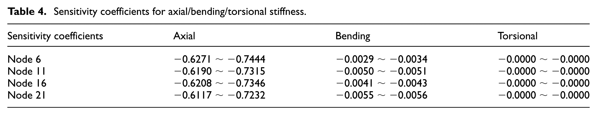
It can be seen from Table 4 that the deflections of nodes 6, 11, 16, and 21 reduced about 0.61%–0.74% with respect to 1% increment in the axial stiffness while that is almost negligible for 1% increment of the bending or torsional stiffness. This indicates that the axial stiffness is the most sensitive parameter for the nodal static deflections. Hence, the Conbim39 element is used to simulate the axial stiffness of the joints in the steel truss bridge model for nonlinear joint model updating. The other two translational and three rotational degrees of freedom are coupled using coupling capability in ANSYS. In order to simulate the model properly, the rotation of the nodal coordinate system is also included. It makes the uncoupled translational degree of freedom sit along the longitudinal axis of the Beam188 element.

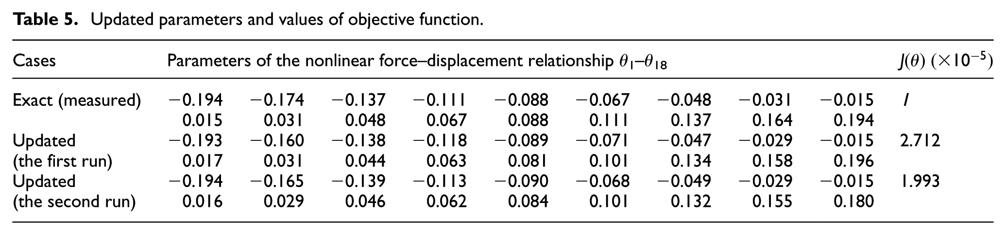
In this case, the force coordinates of these nonlinear force–displacement curve points are uniformly increased from −90 to 90 kN according to the approximated force range. Also, the updating parameters vector is defined as $θ = {θ_{1}, θ_{2}, \dots, θ_{18}}$ with each element representing the displacement coordinate of points to be updated in the nonlinear force–displacement curve. The parameters $θ_{exact}$ (listed in Table 5) are used to calculate the static deflections as the measured responses and the parameters $θ$ to be updated are restricted between 0.7 and 1.3 times of the exact parameters $θ_{exact}$ . The same values of the variables in SA algorithm are used for this updating. Figure 15 shows the convergence of this optimization technique for this example. The function value decreases rapidly during the first few iterations and reaches to a nearly constant value after about 110 iterations. This shows that the convergence speed of the optimization algorithm for this example is also satisfied. The required time varies between 28.5 and 53.5 min and most of the time is spent to carry out the nonlinear static analysis.

Table 5.

Updated parameters and values of objective function.

Cases	Parameters of the nonlinear force–displacement relationship θ₁–θ₁₈									$J (θ) (\times 10^{- 5})$
Exact (measured)	−0.194	−0.174	−0.137	−0.111	−0.088	−0.067	−0.048	−0.031	−0.015	/
Exact (measured)	0.015	0.031	0.048	0.067	0.088	0.111	0.137	0.164	0.194	/
Updated (the first run)	−0.193	−0.160	−0.138	−0.118	−0.089	−0.071	−0.047	−0.029	−0.015	2.712
Updated (the first run)	0.017	0.031	0.044	0.063	0.081	0.101	0.134	0.158	0.196	2.712
Updated (the second run)	−0.194	−0.165	−0.139	−0.113	−0.090	−0.068	−0.049	−0.029	−0.015	1.993
Updated (the second run)	0.016	0.029	0.046	0.062	0.084	0.101	0.132	0.155	0.180	1.993

Figure 15.

The function values with progression of iterations for truss bridge.

The nonlinear joint model updating process has also been run for 20 times due to the randomness. As a result, the nonlinear force–displacement relationship curves of the joint system derived from the nonlinear joint model updating are illustrated in Figure 16. In each figure, the exact force–displacement relationship is compared with that obtained via one run of the model updating program. These figures make it clear that for all the two runs, the updated parameters $θ_{updated}$ match well with the exact parameters $θ_{exact}$ except individual points in the force–displacement curve. The updated coordinate parameters of nonlinear force–displacement relationship curves and the corresponding values of the objective function for the two runs are further listed in Table 5. It can be observed that the novel method presented in this article can be successfully and accurately applied to update the nonlinear joint model parameters.

Figure 16.

Comparisons of nonlinear force–displacement relationship curves between exact and updated results for truss bridge: (a) the first run and (b) the second run.

Figure 17 presents the comparisons of load–deflection relationship curves obtained by analysis of the exact and updated nonlinear joint models. It is manifested that the updated load–deflection curves of the three nodes can match well with that of the exact model. Therefore, the joint system’s nonlinear force–displacement relationship obtained by the presented nonlinear joint model updating program can simulate the behavior of the steel truss bridge correctly.

Figure 17.

Comparisons of nonlinear load–deflection relationship curves of nodes 6/11/21 between exact and updated results: (a) the first run and (b) the 2nd run.

Also, the updated new finite element model is used in the prediction of the structural responses under another new load for validating the efficiency of the updating method. The new concentrated load (F = 80 kN) is simultaneously applied to nodes 11, 31, 143, and 163. The comparisons of load–deflection curves for the three nodes obtained through analysis of the exact and updated nonlinear finite element models are illustrated in Figure 18. It is apparent from this graph that the updated new nonlinear joint model is effective and accurate enough in predicting the behavior subjected to other loads.

Figure 18.

Comparisons of nonlinear load–deflection relationship curves of nodes 6/11/21 between exact and updated results (under the new load): (a) the first run and (b) the second run.

Noise effects

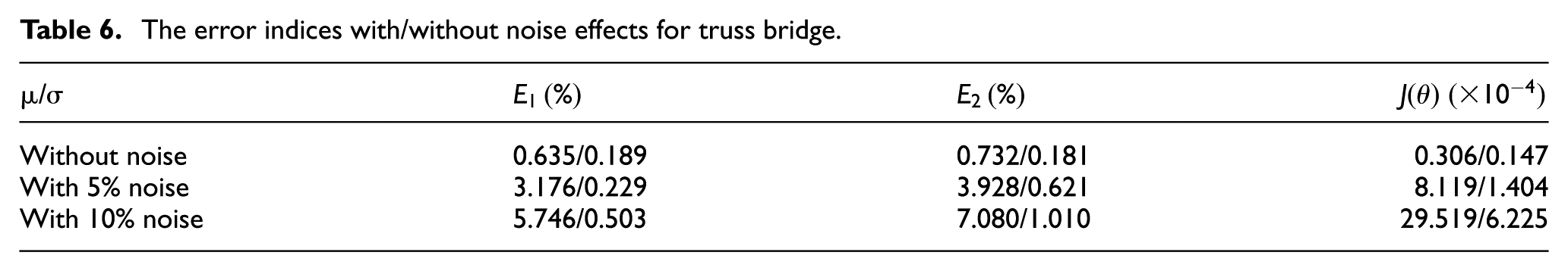
The noise effects have also been studied for this example. Similarly, the simulated deflections with 5% and 10% noise are assumed as the measured responses. Then, the updating program has been run to obtain the proper values of the nonlinear force–displacement parameters. The accuracy of the updated nonlinear model is also evaluated using the defined error indices and the corresponding results are presented in Table 6. It can be known that the proposed model updating method is robust to noise.

Table 6.

The error indices with/without noise effects for truss bridge.

µ/σ	$E_{1} (%)$	$E_{2} (%)$	$J (θ) (\times 10^{- 4})$
Without noise	0.635/0.189	0.732/0.181	0.306/0.147
With 5% noise	3.176/0.229	3.928/0.621	8.119/1.404
With 10% noise	5.746/0.503	7.080/1.010	29.519/6.225

The comparisons of nonlinear load–deflection relationship curves of nodes 6/11/21 between exact and updated results for the cases with noise are also shown in Figure 19. It can be seen that there exists a relatively good fitness between the updated and measured deflections. This reveals the robustness of the proposed nonlinear joint model updating method. Then, a new concentrated load (F = 80 kN) is simultaneously applied to nodes 11, 31, 143, and 163. Figure 20 presents the load–deflection curves obtained through analysis of the exact and updated finite element models. It can be known from Figure 20, the updated new nonlinear joint model can be used to predict the responses subjected to other loads.

Figure 19.

Comparisons of nonlinear load–deflection relationship curves of nodes 6/11/21 between exact and updated results for the case with noise: (a) with 5% noise and (b) with 10% noise.

Figure 20.

Comparisons of nonlinear load–deflection relationship curves of nodes 6/11/21 between exact and updated results (under the new load) for the case with noise: (a) with 5% noise and (b) with 10% noise.

Conclusion

In this article, a novel method for nonlinear joint model updating with structural static data is presented. By performing such method, the joint model parameters have been correctly updated. For the updating technique, the residual between the measured deflections and the analytical deflections is used to create the objective function. A well-known SA algorithm is then introduced to solve the optimization problem. The updating algorithm is first examined by a numerical cantilever beam with nonlinear joint supports. After that, the updating technique is smoothly utilized to a more complex numerical steel truss bridge with nonlinear joint force–displacement relationship. The optimization performs well in both of the two numerical cases. The obtained results indicate that the nonlinear joint model parameters can be successfully updated and the updated model can further forecast the actual deflection of the nonlinear system.

In future study, this method will be tested on several more complicated cases such as experimental structures. For practical application, the joint system may show more complicated nonlinear behaviors; therefore, the consideration of more appropriate nonlinear joint models will be essentially necessary. Another urgent task is to improve the nonlinear model updating algorithm as well as the measuring and testing technique. Some other optimization algorithms combined with higher-order sensitivity are worth investigating. A more detailed analysis on the updating of dynamic nonlinear behavior for joint system should also be focused on.

Footnotes

Acknowledgements

The results and opinions expressed in this article are those of the authors only and they do not necessarily represent those of the sponsors.

Academic Editor: Simon Laflamme

Declaration of conflicting interests

The author(s) declared no potential conflicts of interest with respect to the research, authorship, and/or publication of this article.

Funding

The author(s) disclosed receipt of the following financial support for the research, authorship, and/or publication of this article: Financial support to complete this study was provided in part by the National Natural Science Foundation of China under grant nos 51578206 and 51278163, and by “The Fundamental Research Funds for the Central Universities.”

References

Ahmadian

Mottershead

Friswell

. Joint modeling for finite element model updating. In: Proceedings of the 14th international modal analysis conference (IMAC), Dearborn, MI, 12–15 February 1996, pp.591–596. Bethel, CT: Society for Experimental Mechanics, Inc.

Mackerle

Finite element analysis of fastening and joining: a bibliography (1990–2002). Int J Pres Ves Pip 2003; 80: 253–271.

Ahmadian

Mottershead

James

. Modelling and updating of large surface-to-surface joints in the AWE-MACE structure. Mech Syst Signal Pr 2006; 20: 868–880.

Dias

AMPG

Van de Kuilen

Lopes

. A non-linear 3D FEM model to simulate timber-concrete joints. Adv Eng Softw 2007; 38: 522–530.

Mayer

Gaul

Segment-to-segment contact elements for modeling joint interfaces in finite element analysis. Mech Syst Signal Pr 2007; 21: 724–734.

Bograd

Reuss

Schmidt

. Modeling the dynamics of mechanical joints. Mech Syst Signal Pr 2011; 25: 2801–2826.

Gaul

Lenz

Nonlinear dynamics of structures assembled by bolted joints. Acta Mech 1997; 125(1–4): 169–181.

Girão Coelho

Simões da Silva

Bijlaard

FS.

Finite-element modeling of the nonlinear behavior of bolted T-stub connections. J Struct Eng 2006; 132: 918–928.

Schwingshackl

Di Maio

Sever

. Modeling and validation of the nonlinear dynamic behavior of bolted flange joints. J Eng Gas Turb Power 2013; 135: 122504.

10.

Khorsandnia

Valipour

Crews

Nonlinear finite element analysis of timber beams and joints using the layered approach and hypoelastic constitutive law. Eng Struct 2013; 46: 606–614.

11.

Yang

Fan

Lin

CS.

Joint stiffness identification using FRF measurements. Comput Struct 2003; 81: 2549–2556.

12.

Cunha

Foltête

Bouhaddi

Evaluation of stiffness of semi-rigid joints in pultruded profiles from dynamic and static data by using model updating technique. Eng Struct 2008; 30: 1024–1036.

13.

Jalali

Ahmadian

Mottershead

JE.

Identification of nonlinear bolted lap-joint parameters by force-state mapping. Int J Solids Struct 2007; 44: 8087–8105.

14.

Eriten

Kurt

Luo

. Nonlinear system identification of frictional effects in a beam with a bolted joint connection. Mech Syst Signal Pr 2013; 39: 245–264.

15.

Mehrpouya

Graham

Park

SS.

FRF based joint dynamics modeling and identification. Mech Syst Signal Pr 2013; 39: 265–279.

16.

Iranzad

Ahmadian

Identification of nonlinear bolted lap joint models. Comput Struct 2012; 96: 1–8.

17.

Alamdari

Samali

. Nonlinear joint model updating in assembled structures. J Eng Mech 2013; 140: 04014042.

18.

Lei

Chen

. Damage identification of frame structures with joint damage under earthquake excitation. Adv Struct Eng 2014; 17: 1075–1088.

19.

Davoodi

Amiri

Gholampour

. Determination of nonlinear behavior of a ball joint system by model updating. J Constr Steel Res 2012; 71: 52–62.

20.

ANSYS user’s manual (revision 11.0), 2007.

21.

Zhang

Der Kiureghian

Dynamic response sensitivity of inelastic structures. Comput Method Appl M 1993; 108: 23–36.

22.

Kleiber

Hien

Antúnez

. Parameter sensitivity in nonlinear mechanics: theory and finite element computations. Hoboken, NJ: John Wiley & Sons, 1997.

23.

Conte

JP.

Finite element response sensitivity analysis in earthquake engineering. In: Hu

Spencer

(eds) Earthquake engineering frontiers in the new millennium, 2001, pp. 395–401. Lisse: CRC Press.

24.

Jaishi

Ren

WX.

Structural finite element model updating using ambient vibration test results. J Struct Eng 2005; 131: 617–628.

25.

Houck

Joines

Kay

MG.

A genetic algorithm for function optimization: a MATLAB implementation. NCSU-IE TR, 1995, http://citeseerx.ist.psu.edu/viewdoc/download?doi=10.1.1.22.4413&rep=rep1&type=pdf

26.

Basheer

Hajmeer

Artificial neural networks: fundamentals, computing, design, and application. J Microbiol Meth 2000; 43: 3–31.

27.

Lee

Geem

ZW.

A new structural optimization method based on the harmony search algorithm. Comput Struct 2004; 82: 781–798.

28.

Bertsimas

Tsitsiklis

Simulated annealing. Stat Sci 1993; 8: 10–15.

29.

Wang

Xin

Ren

WX.

Nonlinear structural model updating based on instantaneous frequencies and amplitudes of the decomposed dynamic responses. Eng Struct 2015; 100: 189–200.

30.

Wang

Xin

Ren

WX.

Nonlinear structural joint model updating based on instantaneous characteristics of dynamic responses. Mech Syst Signal Pr 2016; 76: 476–496.

31.

Ingber

Very fast simulated re-annealing. Math Comput Model 1989; 12: 967–973.

32.

Levin

Lieven

NAJ

. Dynamic finite element model updating using simulated annealing and genetic algorithms. Mech Syst Signal Pr 1998; 12: 91–120.

33.

Jeong

Lee

JJ.

Adaptive simulated annealing genetic algorithm for system identification. Eng Appl Artif Intel 1996; 9: 523–532.

34.

Astroza

Nguyen

Nestorović

Finite element model updating using simulated annealing hybridized with unscented Kalman filter. Comput Struct 2016; 177: 176–191.

35.

Moore

MATLAB for engineers. Upper Saddle River, NJ: Prentice Hall, 2014.

36.

Zhang

Chang

TYP

. Finite element model updating for structures with parametric constraints. Earthq Eng Struct D 2000; 29: 927–944.

37.

Zhang

Chang

TYP

Chang

CC.

Finite-element model updating for the Kap Shui Mun cable-stayed bridge. J Bridge Eng 2001; 6: 285–293.

Nonlinear joint model updating using static responses

Abstract

Keywords

Introduction

Theoretical background

Nonlinear joint model

Sensitivity analysis

Objective function

Optimization technique

Numerical verification

Simulated cantilever beam with nonlinear joint supports

Model description

Nonlinear joint model updating

Noise effects

Simulated steel truss bridge

Model description

Nonlinear joint model updating

Noise effects

Conclusion

Footnotes

Acknowledgements

Declaration of conflicting interests

Funding

References