
Abstract
A simplified variational iteration method is proposed to solve high-order homogeneous or nonhomogeneous linear ordinary differential equation and ordinary differential equation eigenvalue problems more efficiently and conveniently. The simplification includes two aspects: (1) explicitly deducing the general form of the differential equation for the identification of the general Lagrange multiplier while avoiding the complexity of variational calculations during identification and (2) simplifying the iterative expressions to reduce the computational work of each iteration. Three ordinary differential equations in mechanics are solved by this simplified variational iteration method, which proves that it is valid and more concise than traditional methods. To make the method more practical, it is suggested that some complicated analytical derivations be executed numerically, thereby achieving a simplified semi-analytical variational iteration method that can be easily implemented by computer programs. The method is then used to numerically solve two complex ordinary differential equation problems derived from the continuum analysis of tall building structures: a sixth-order nonhomogeneous ordinary differential equation with complex boundary conditions and a sixth-order ordinary differential equation eigenvalue problem. Numerical computer programs are developed for these two problems, and corresponding examples are provided to verify the accuracy and efficiency of the simplified variational iteration method in solving complex ordinary differential equation problems.
Keywords
Introduction
Differential equations are widely used to describe various mechanical problems, 1 thus making the method used to solve them an important issue in many cases. For low-order and simple differential equations, it is easy to obtain analytical solutions; however, for high-order or complicated ones, analytical solutions are difficult to obtain or may not even exist. Numerical approaches are therefore normally employed in practice to obtain usable results, especially in engineering. 2 Ordinary differential equations (ODEs) 3 are equations with only one independent variable and can be mainly divided into two types according to the boundary conditions: initial value problems (IVPs) and boundary value problems (BVPs). Between these two types of problems, the solution of BVPs is more complicated because the boundary conditions are defined at different points. The commonly used numerical solution methods for BVPs are the shooting method, Galerkin method, finite difference method, finite element method, 4 and so on. These methods are all capable of solving ODEs, but do have some drawbacks. The shooting method involves solving the BVP’s approximate IVP several times, which could be time-consuming for complicated problems. The Galerkin’s method requires finding a series of trial functions that are compatible with the boundary conditions, but these functions are not always easy to determine. As for the finite difference method and finite element method, the accuracy of the solution is heavily dependent on the density or quality of the mesh. What’s more, these methods are all approximate methods, even for linear ODEs.
Variational iteration is a relatively new method for solving differential equations that is theoretically accurate with simple concepts and fast convergence. It is derived from the general Lagrange multiplier method used for solving nonlinear equations in quantum mechanics, 5 which was modified by He5–8 and Biazar et al. 9 into an iteration method named the variational iteration method (VIM). The VIM is in fact a general form of the Newton–Raphson iteration method. 5 Moreover, H Jafari 10 has recently proved that when the highest derivative term is considered the linear part in the VIM while solving nonlinear differential equations, the VIM is equivalent to the well-known classical successive approximations method. The VIM provides an effective means for solving differential equations, large linear systems, and so on and has been used to solve various differential equations in different disciplines, such as the Fokker–Planck equation11–13 and Boltzmann equation 14 in statistical mechanics, fractional partial differential equations in fluid mechanics, 15 nonlinear wave equations,16–18 partial differential equations for water waves, 19 variational problems, 20 nonlinear equations in heat transfer,21,22 free vibration problems of Euler–Bernoulli beams 23 and marine risers, 24 and eigenvalue problems of Sturm–Liouville differential equations 25 and nonlinear oscillators.26–28
In this study, the VIM is simplified to solve high-order linear ODEs and ODE eigenvalue problems more conveniently and practically. First, the general form of the differential equation for identifying the general Lagrange multiplier is explicitly given, and then the iterative formulae are simplified for linear ODEs. In addition, integral expressions are suggested to be performed numerically in order to avoid complicated analytical derivations and make the method more convenient for numerical computer programming. Finally, several ODEs are selected for solving by the simplified VIM to verify its validity and efficiency.
Simplification of VIM
In general, an ODE can be expressed in the following form

where F denotes the differential operator of the ODE.
Now, suppose that the solution of the above ODE can be expressed in an iterative form as
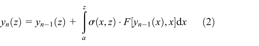
where
The real solution is denoted by

Substituting the above equation in equation (2), we have

Supposing that

Provided that
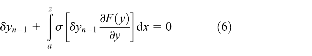
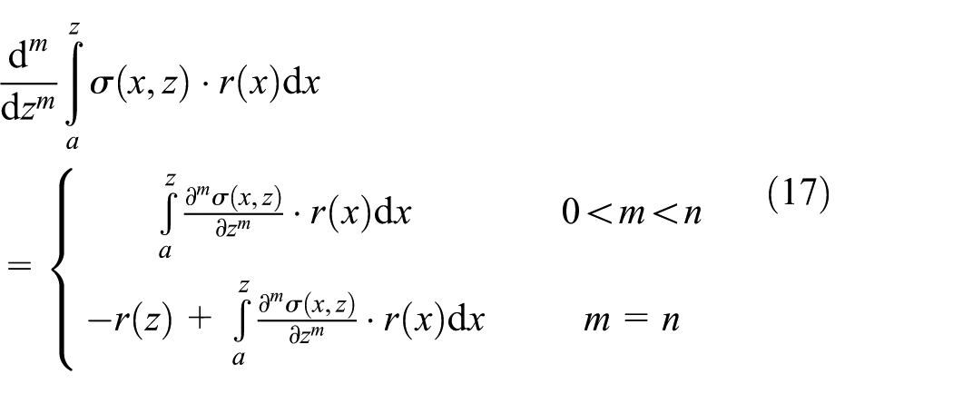
holds, the discrepancy after n iterations
Equation (6) can therefore be used to identify the optimum generalized Lagrange multiplier
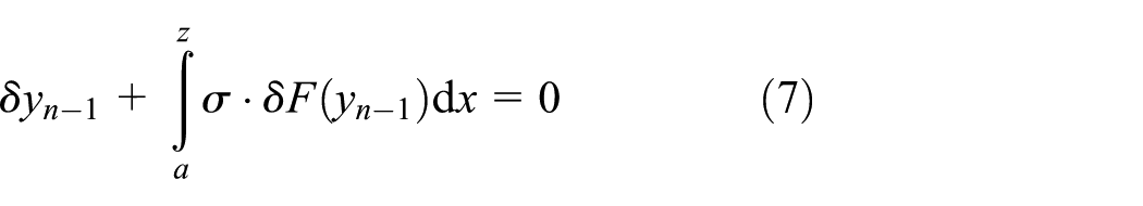
If we now consider a special case in which

That is

The above formula is the iteration formula of the famous Newton–Raphson method for solving nonlinear equations, which means that the VIM can be regarded as a general form of the Newton–Raphson method or that the Newton–Raphson method is a particular case of the VIM. In this manner, the validity and feasibility of the VIM is also verified from a unique perspective.
When the operator F is complicated, it is difficult to obtain the expression for

where L is a simple linear operator (so simple that the analytical solution of

Equation (11) produces several stationary conditions that can be treated as a differential equation (equation (12)) together with the corresponding boundary conditions (equation (13)) with respect to the generalized Lagrange multiplier


where
Later,
Based on the above derivations, the operator L and Lagrange multiplier


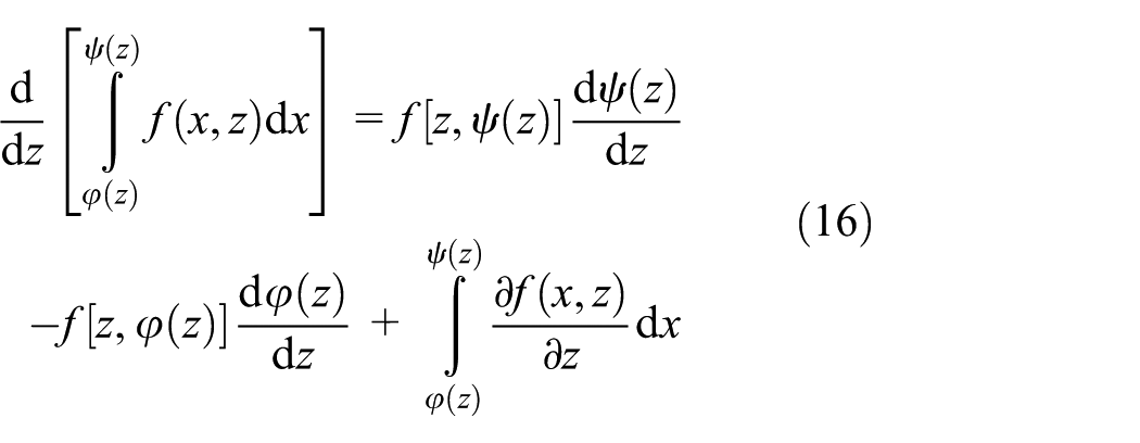
In view of the derivation formula for the uncertain limit integral given below
We can obtain a new property of
Because the linear operator L can be expanded as

We obtain

That is

We now define a new symbol

where

Supposing that N is also a linear operator, as per equation (2), we get

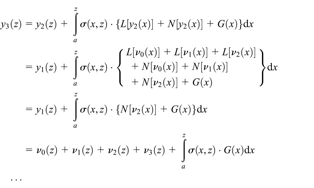
Analogically, the ith iterative solution can be expressed as
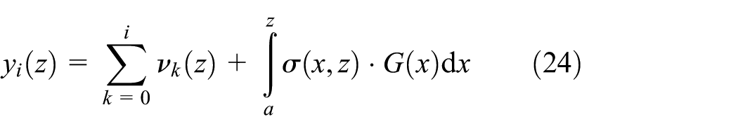
The above expression means that iterations need not be carried out using equation (2), but instead only
From equations (21) and (24), we can also infer that when

For IVPs, the initial solution
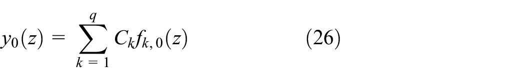
where
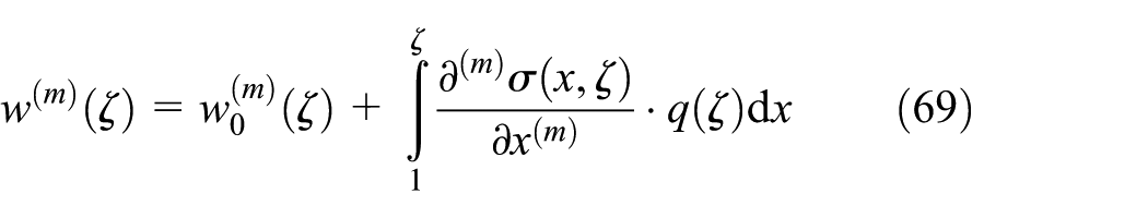
The ith iterative solution

where

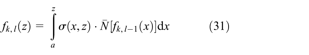
Equation (27) divides the iterative solution into several components, each of which can be calculated independently (equation (28)), so the undetermined coefficients can be ignored during the iterations. In this manner, the derivation in every iterative step is kept brief and simple, making it easy to obtain the numerical approaches involved.
As for the eigenvalue problems of ODEs, the operator N can usually be written in the following form

By repeating the deduction in equation (23), the solution after the ith iteration can be obtained as

where
Verification of simplified VIM
Here, three simple but classical problems will be solved using the simplified VIM to demonstrate the solution procedure and verify the validity of the simplification.
Problem I: Forced vibration of undamped single-degree-of-freedom system
The differential equation of forced vibration for an undamped single-degree-of-freedom (SDOF) system is 27

whose initial conditions are

According to equation (10), the operators can be identified as

Substituting the above equations in equations (12) and (13), we have

The generalized Lagrange multiplier

Forcing

Because

Equation (38) is the well-known Duhamel integral or the solution of the vibration of an SDOF system under arbitrary dynamic loads. This proves that the identified generalized Lagrange multiplier based on equations (12) and (13) is rational, and that the simplified VIM is valid and capable of solving IVPs.
Problem II: Cantilever (Euler–Bernoulli beam) under distributed transverse load
If the distributed transverse load is set to

where

The analytical solution of equation (39) can be obtained by simply integrating the equation four times

To now try and solve equation (39) using the simplified VIM, the operators should first be identified

Then, based on equations (12) and (13), we have

which yields the generalized Lagrange multiplier

Considering

Because

The undetermined coefficients can be obtained using the boundary conditions in equation (40), as per the following

If we substitute the value of the above coefficients in equation (46), the expression obtained will be the same as that in equation (41). This example proves that the simplified VIM is capable of solving BVPs.
Problem III: Free vibration of cantilever (Euler–Bernoulli beam)
The eigenvalue differential equation of transverse free vibration of a cantilever (Euler–Bernoulli beam) is

The boundary conditions are the same as those in equation (40). The precise results of eigenvalues are the roots of the following equation

The numerical values of the accurate eigenvalues (the first two orders) are

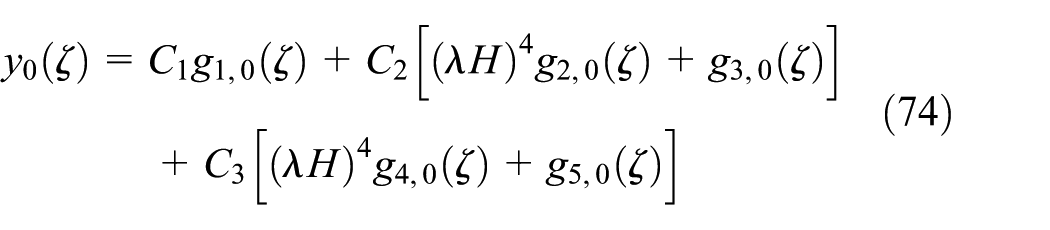
When using the VIM, the operator L is chosen as

The other operators are can then be identified as

Because
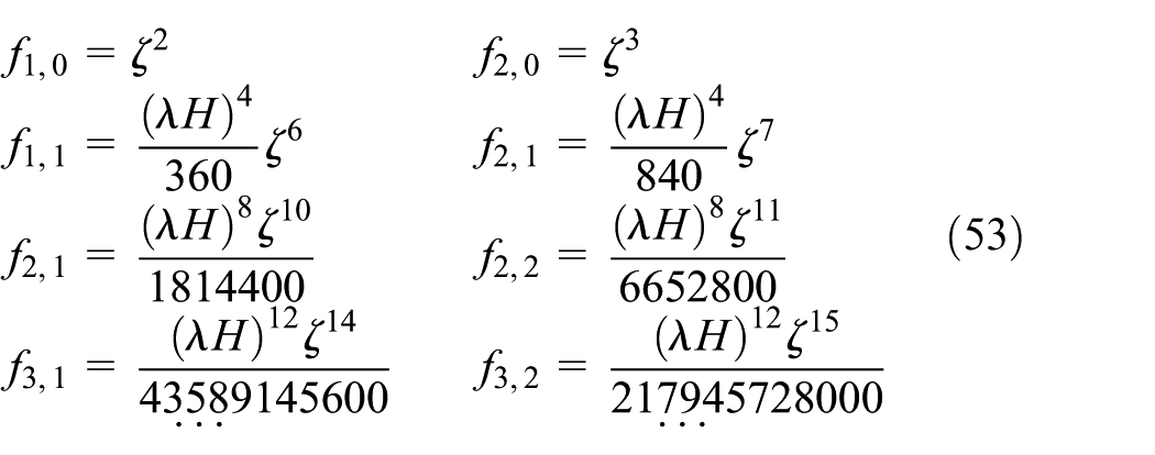
Substituting the above equations, we get
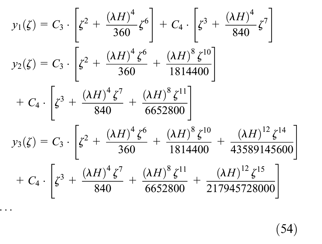
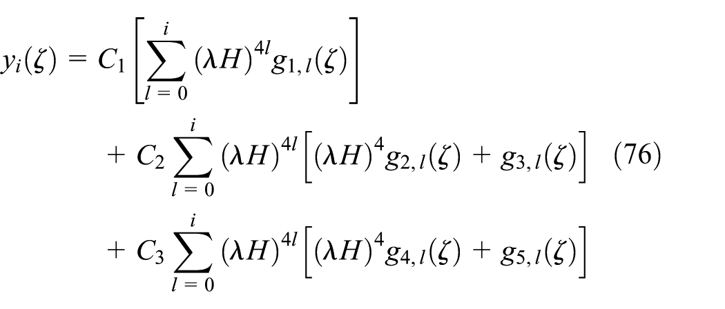
Considering the boundary conditions at

The numerical roots of the above equations (Table 1) indicate that the iterative result will converge step-by-step to an accurate solution as the iteration count increases. Thus, although the simplified VIM can also solve the eigenvalues of ODEs, the expression of the solution will become increasingly complicated (i.e. the number of terms may grow exponentially) as the iterations proceed. To make the application of the method more convenient, we suggest that the integrals and differentials in equation (28) be calculated by numerical methods instead of analytical derivation, which would make the method a semi-analytical but practical one. In addition, numerical differentials should be avoided because these make it difficult to guarantee accuracy.
Eigenvalues of free vibration of cantilever (Euler–Bernoulli beam) calculated by simplified variational iteration method.

Application of simplified VIM to complicated ODE problems
In this section, two complicated ODE problems are solved by the proposed VIM method in order to verify and investigate the feasibility and convenience of the method.
Problem description
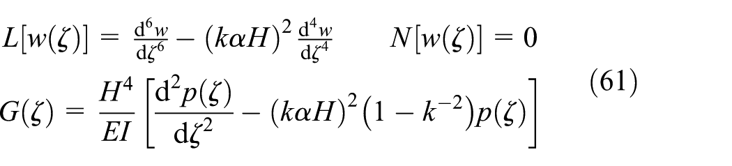
In the classic theory of tall building analysis, structures are usually idealized as a continuous sandwich cantilevers 30 so that their static and dynamic behavior can be described using differential equations.
The following differential equations are those used to describe a tall building structure under static load and free vibration, respectively 30

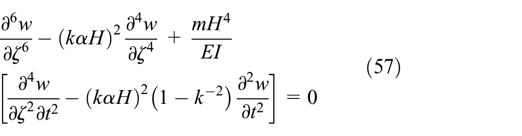
where,
Equation (57) can be changed into an ODE by spectral transformation in order to solve the free vibration eigenvalues of a tall building structure

where
The corresponding boundary conditions of the ODE (56) are

and these are the boundary conditions for the ODE (58)

The general procedure used to obtain the analytical solution of the eigenvalue differential equation (equation (58)) is as follows. First, treat the equation as a normal homogeneous ODE with constant coefficients and find its general solution (include six integration constants
Solution of sixth-order nonhomogeneous ODE
As mentioned above, the first task involved in solving differential equations by the VIM is to identify the generalized Lagrange multiplier. Before performing this task, the operators in equation (10) should be determined in comparison with equation (56) as follows
Then, the recognition equation of the generalized Lagrange multiplier can be obtained based on equations (12) and (13)

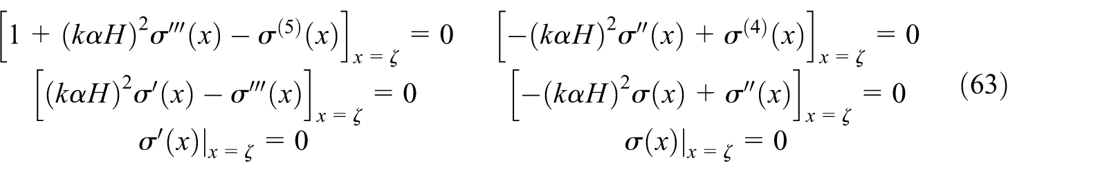
which yields

Considering

Because

where the expressions for
A linear system of equations with respect to the undetermined coefficients

where

The values of
A computer program based on the above derivation named ODETB (solver for an ODE of a tall building structure under static loads) was developed using Julia Language, 31 which is a high-level, high-performance, dynamic programming language for technical computing. This ODETB is capable of solving ODEs (such as equation (56)) for tall building structures under arbitrary lateral loads.
To verify the ODETB, a simple example is presented wherein a tall building is carrying a distributed inverted triangle load

where
Relative errors of ODETB results compared with analytical solutions.

Solution of sixth-order ODE eigenvalue problem
Comparing equation (58) with equations (10) and (29), the operators can be identified as

The generalized Lagrange multiplier is same as that in equation (64), and the initial solution is also same as that in equation (65) because the operator L in the above equation is identical to the one in equation (61). To make the solution process simpler, the new initial solution is determined using the boundary conditions at

where

Because there is an unknown variable
where

The ith iterative solution can then be determined on the basis of equations (30) and (74) as
where

The differential involved in equations (77) and (60) can be computed as follows according to equation (17)

where m is the order of the differential and m < 6.
A linear system of equations with respect to the undetermined coefficients

where


According to Cramer’s rule, the following equation must hold true if the above linear system has non-zero solutions

It can be predicted that equation (82) can be arranged as a polynomial equation of
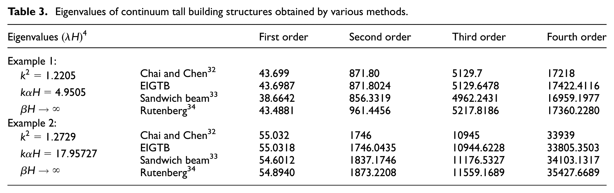
Based on the above discussions, we have developed a corresponding computer program using Julia to solve the ODE eigenvalue problems of tall buildings by the semi-analytical VIM. To validate this program, which is called EIGTB (solver for a ODE eigenvalue problem of a tall building structure for free vibration), two examples referred to by Chai and Chen 32 were recomputed using EIGTB and two other approximate methods: the equivalent sandwich beam method 33 and Rutenberg’s 34 method. The numerical results of the eigenvalues of these examples are listed in Table 3, and the eigenmodes are shown in Figure 1 (EIGTB results were obtained using 50 integral points, involving only 6 iterations). These results confirm that the semi-analytical VIM and EIGTB program proposed in this article are valid and accurate.
Eigenvalues of continuum tall building structures obtained by various methods.
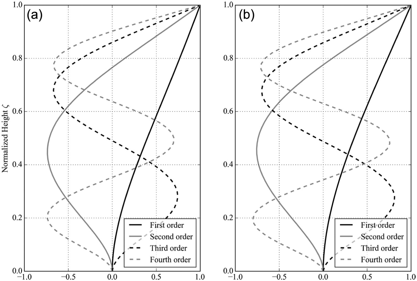
Eigenmodes of continuum tall building structures solved by EIGTB: (a) example 1 and (b) example 2.
Conclusion
In this study, the original VIM is simplified and modified into a semi-analytical method to solve high-order complicated ODEs in a more convenient and practical manner.
The general form of the differential equation with respect to the general Lagrange multiplier is explicitly stated, which facilitates the identification of the general Lagrange multiplier.
For linear ODEs, the operator L can be eliminated during the iterative solving procedure, which reduces the iterative computational burden.
The integrals involved in the iterations are suggested to be calculated numerically for practical use.
The simplified VIM has been proven to be an efficient and practical method for solving complicated ODEs (including eigenvalue ODEs), and the implementation of this method is both simple and convenient.
Footnotes
Academic Editor: Mohana Muthuvalu
Declaration of conflicting interests
The author(s) declared no potential conflicts of interest with respect to the research, authorship, and/or publication of this article.
Funding
The author(s) disclosed receipt of the following financial support for the research, authorship, and/or publication of this article: This study was supported by the National Natural Science Foundation of China (grant no. 51308418 and 51478356), by the Shanghai Committee of Science and Technology (grant no. 10DZ2252000), and by the Sichuan Department of Science and Technology (grant no. 2016JZ0009).