
Abstract
Bridge structures in service are subjected to long-term ambient environments and continuously increasing traffic demands; therefore, the physical quantities of the existing bridge structures are subjected to changes in both time and space. Through health monitoring for bridges, the data of the load effects of bridge structures, including strain, stress, deflection, and so on, of the specified structural components or structures, can be obtained. The novel monitoring systems installed in bridge structures contain sensors providing a large amount of monitored data. Proper processing of the continuously provided monitored data is one of the main difficulties in the field of structural health monitoring for time-dependent reliability prediction of structural components and/or structures. Under the actions of the common random sources of the time-dependent input load data, the time-dependent nonlinear correlation will exist among the time-dependent output load effect data. The Bayesian dynamic linear models are introduced to predict the time-dependent output variables and model the time-dependent nonlinear correlation coefficients between them. Then, the Gaussian copula–Bayesian dynamic linear models are built based on the Gaussian copula theory and the time-dependent correlation coefficients. The models can better and more feasibly predict the future reliability of bridge structures. Finally, an actual application example is provided to illustrate the feasibility and application of the built Gaussian copula–Bayesian dynamic linear models for structural reliability prediction.
Keywords
Introduction
The time-dependent structural reliability formula is often expressed in terms of a vector of basic random variables characterizing uncertainties in quantities such as time-variant resistances (time-variant allowed load effect caused by structure degradation) and time-dependent load effects which are usually correlated with each other. For example, peak and permanent displacements of a system subjected to earthquake loading are correlated with each other. 1 Uncertainty in structural reliability analysis2–6 and the dependence modeling7–9 have caused more attentions by the planners at home and abroad. But how to make reasonable uncertainty model is rarely studied in the analysis of structural time-dependent reliability.
To predict structural time-variant reliability reasonably, the complete probability information such as the time-dependent joint cumulative distribution function (CDF) and the time-variant joint probability density function (PDF) of the random time-variant vector should be known. 10 In engineering practice, however, the joint PDF cannot be often obtained due to the limited data. In most practical applications, only the marginal PDFs and the covariance matrix are available, so the incomplete statistical data are quite commonly available.11–13 Furthermore, the marginal distributions are often nonnormal distributions, and it is accepted that the modeling and simulation of the non-Gaussian random vectors are challenging problems. 14 However, the nonnormal distributions could be transferred into the combination of a few normal distributions based on such limited information. So, the joint PDFs could be approximately defined. Consequently, an evaluation of the failure probability is possible through modeling and constructing the approximated multivariate distribution based on incomplete statistical data.
It is evident that the time-dependent reliability of an individual component cannot represent the time-variant reliability of the entire structural system. 15 So, it is of practical interest to reasonably determine the time-dependent reliability of the entire structural system. In addition, the time-dependent nonlinear correlation between failure modes of the entire structural system should be considered. And the copula function can handle with the correlation modeling, and the application of copulas in modeling temporal dependence of time series data appears to be a recent phenomenon. 16 Dynamic or time-varying copula models for bivariate time series data have been studied by Patton, 17 Dias and Embrachts, 18 and Van den Goorbergh et al., 19 and Joe 7 studied Markov time series using copulas with constant parameter, but little is used in structural system reliability analysis. With these in mind, time-dependent Gaussian copulas for modeling the time-dependent joint distributions on the time-dependent system reliability could be explored and are the topic of the present research.
The objective of this study is to predict the time-dependent reliability of bridge structures considering time-variant nonlinear correlation between failure modes based on the built Gaussian copula–Bayesian dynamic linear models (BDLMs), to achieve this goal; this article is organized as follows: In section “Gaussian copula theory,” the Gaussian copula theory is described; especially, the concepts of Pearson correlation coefficient is introduced briefly. In section “Gaussian copula-BDLMs,” one BDLM and its probability recursion processes are provided to predict the relevant information, and the predicted time-variant correlation coefficient formulas between different BDLMs are presented for constructing the time-dependent Gaussian copula function. In section “The modeling processes of Gaussian copula-BDLMs,” one kind of correlation coefficient-based Gaussian copula-BDLMs and their modeling processes are given in detail. In section “Reliability prediction of structural system considering the nonlinear correlation between failure modes,” the built Gaussian copula-BDLMs are used to predict the structural time-dependent reliability. One numerical example is provided to illustrate the feasibility and application of the built models in section “A numerical example: reliability prediction of Yitong River Bridge.”
Gaussian copula theory
Sklar’s theory
20
clearly indicated that given random variables

According to equation (1), the joint PDF of the random variable

where

If

where
Equation (4) reveals how to construct the copula function of a multivariate distribution with given marginal distributions. It follows from the probability integral transform that the random variables

According to equations (1)–(5), the copula function organically combines each marginal distribution functions with the multivariate joint distribution functions; therefore, it not only considers the dependence among random variables but also simplifies the probability modeling process for multivariate random variables.
According to the construction method of the elliptical copulas, Gaussian copula function, belonging to the frequently used elliptical copula family, is defined as the joint normal CDF of multiple standard normal variables. For two-dimensional copula function, the corresponding CDF C and PDF c are, respectively


where
With equations (6) and (7), the joint CDF and joint PDF of


As far as the Gaussian copula function is concerned, the main problem is to determine the correlation parameter
Pearson correlation coefficient
The Pearson product–moment correlation is also called linear correlation.
23
Let

where
Based on the sampled data of

where
With equation (10), the relation 24 between linear correlation coefficient and correlation parameters of Gaussian copula function can be expressed with

where
Based on equations (10) and (11), the linear correlation coefficients between
According to equations (10) and (11), if the marginal distributions of
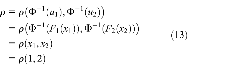
With equation (13), the correlation parameters of Gaussian copula function can be solved. Due to the special characteristics of Gaussian copula function, namely, the marginal distributions of
Gaussian copulas are able to capture symmetric dependence structures (including positive correlation and negative correlation) among random variables, which are shown in Figures 1 and 2.

(a) The PDF plot for a Gaussian copula PDF, (b) the contour plot, and (c) the PDF plot on the antidiagonal line

(a) The PDF plot for a Gaussian copula PDF, (b) the contour plot, and (c) the PDF plot on the diagonal line x1 = x2.
Gaussian copula function has been widely applied in static copula theory, but the time-dependent correlation modeling for the dynamic time series cannot be well handled with the static copula theory. In order to reasonably assess the structural time-variant reliability, the dynamic Gaussian copula function with time-dependent correlation parameters, namely, Gaussian copula-BDLMs, is built in this article, which can analyze the time-variant nonlinear correlation between different time series.
Gaussian copula-BDLMs
BDLMs
BDLMs are the predicting approaches based on a philosophy of information updating 25 which define a dynamic model system of time series processes that can incorporate all useful monitored information into the model to update the prediction model. The BDLMs include a state equation, an observation equation, the initial information, and the time-dependent probability recursion processes based on Bayesian method. The state equation, which is very critical to determine, shows changes of the system with time and reflects inner dynamic changes of the system and random disturbances. The observation equation expresses the relationship between the measured data and the current state parameters of the system.
The BDLMs mean that the observation equation and the state equation are both linear. First-order autoregression (AR(1)) model is adopted to build the state equations in this article.
BDLMs based on AR(1) model
The time series model, AR(1) model, 26 can be used to predict the future data of time t only based on the monitored data of time t, so that the AR(1) model can be applied to simply build the BDLMs.
1. AR(1) model

where
2. State equation based on equation (14): Based on equation (14), the state variable keeps in line with the trend changes of monitored data; therefore, the transformed approximate state equation of monitored data is
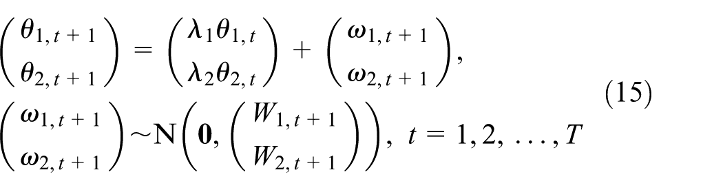
where
3. Transferred BDLMs based on AR(1) model: According to the definition of BDLMs,
25
based on AR(1) model, for each time t, the general and easy form of the dynamic linear models is defined as follows: Observation equation
State equation
Initial information


where
Probability recursion of BDLMs
The probability recursion processes of BDLMs based on AR(1) model
1. The state posteriori distribution at time t: For the mean mi,t and the variance Ci,t, there is

2. The state priori distribution at time t + 1

where
3. One-step prediction distribution at time t + 1
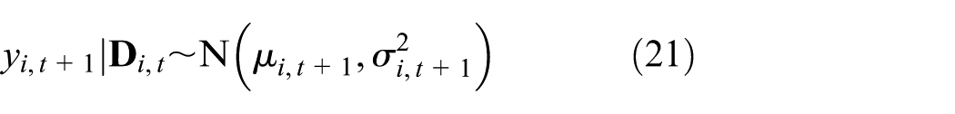
where
4. The state posteriori distribution at time t + 1

where
Determination of the main probability parameters of BDLMs
For the BDLMs, the main probability parameters are Vt+1, Wt+1, mt, and Ct. The method of determining the main probability parameters is described in the following.
In this article, the interval period of model updating is 1 day; Vt+1 is estimated with the variance of differences between fitted trend data and monitored data. According to the researches,25,27Wt+1 can be solved with equation (23)

where
If the initial state data follow the lognormal distribution, then the state data can be transformed into a quasi-normal distribution
28
with equations (24) and (25), the distribution parameters are, respectively,


where g(·) is the actual fitted PDF of the sample data (lognormal PDF), G(·) is the actual probability distribution function (lognormal probability distribution function), and G(x0) = 0.05.
If the initial state data follow the other distributions, then the distribution can be approximately obtained as follows:
1. With estimation method of kernel density, the actual distribution function

2. Since any set of data can be fitted by a few normal distributions, namely

where
3. The weights and distribution parameters of the fitted normal distributions can be obtained with the least residual error quadratic sum method ordinary least squares (OLS), namely

where
Therefore, the distribution parameters (mean and variance) of state at time t are, respectively


Correlation parameters of Gaussian copula-BDLMs
This article takes the two-dimensional random variables as the example, based on the BDLMs, the time-variant correlation parameters of Gaussian copula function is computed through Pearson linear correlation coefficients:
1. Time-variant correlation parameters of Gaussian copula function based on Pearson linear correlation coefficients: For the corresponding BDLMs to two different monitored variables

Because two predicted random variables both follow normal distributions, with equation (13), time-variant correlation parameter

For different BDLMs, the marginal distributions of the predicted random variables
Correlation parameters of Gaussian copula function considering the correlation between the predicted random variables based on the AR(1)-BDLMs
1. Time-variant correlation parameters of Gaussian copula function based on Pearson linear correlation coefficients: Suppose that the predicted random variables

Furthermore, the corresponding correlation parameters of Gaussian copula function at time t + 1 is

The modeling processes of Gaussian copula-BDLMs
The modeling processes of Gaussian copula-BDLMs based on the Pearson correlated coefficients
With equations (33) and (34), the correlation parameters of Gaussian copula function at time t + 1 is

Then, based on the BDLMs of two predicted random variables

Let

Then, the Gaussian copula-BDLMs can be expressed as

where
Reliability prediction of structural system considering the nonlinear correlation between failure modes
Some structure has two failure modes, and the corresponding performance functions are

where
The failure probability, when the two failure modes meantime occurred, is
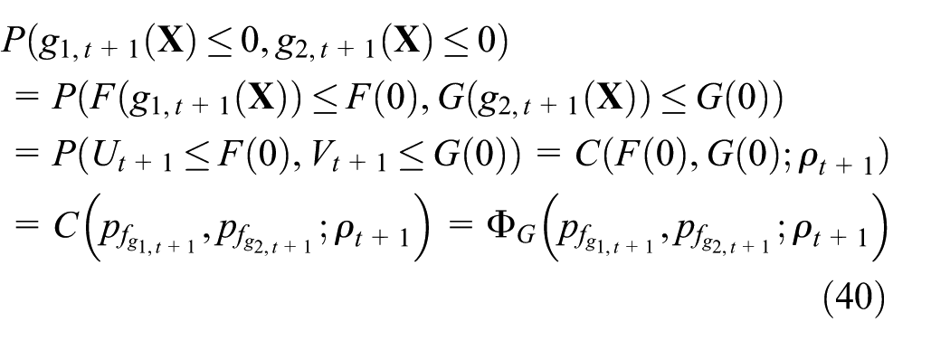
where

First, with equation (13), the following can be solved

Then, with equations (33) and (34), the correlation parameters

where
Failure probability of multiple-dimensional series system can be solved based on equation (43), by computing the time-variant correlation parameter matrix and the marginal distributions of all the predicted random variables based on BDLMs.
A numerical example: reliability prediction of Yitong River Bridge
Yitong River Bridge over Yitong River was built in 2009 in the city of Changchun, China. It is a flying swallow profiled concrete-filled steel tube arch bridge which is at no. 102 National Highway in Changchun. The main bridge of Yitong River Bridge is 260 m, and the main span is 158 m, which is shown in Figures 3–5. Details of this bridge are provided in Qu and Xie 29 and Zhao. 30 The monitoring program for this bridge included the assessment of the stain and deflection of specified structural components.

Yitong River bridge (Changchun city from Jilin Province in China).

The layout of Yitong River Bridge.

Schematic diagram of Yitong River Bridge.
The everyday extreme deflections of the middle parts for upper stream and lower stream middle spans are monitored for 45 days, which are shown in Table 1. The distribution parameters of the allowed deflection about the middle parts of upper stream and lower stream main spans are, respectively,
Monitored and predicted information for mid-span deflection of upper stream and lower stream main spans.

The performance functions about the middle deflections of the upper stream and lower stream main spans are, respectively
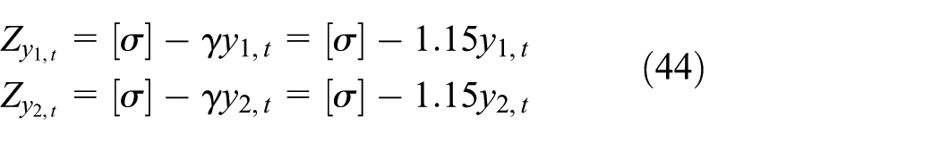
where
Observation equation

State equation

Initial information

where
Based on section “Gaussian copula-BDLMs,” the monitored deflection data, predicted deflection data, and the time-dependent correlation parameters of the built Gaussian copula functions are, respectively, shown in Table 2 and Figures 6–9.
Reliability indices and failure probability of upper stream and lower stream main spans.


Monitored and predicted upper stream deflection.

Monitored and predicted lower stream deflection.

Prediction precision of upper stream and lower stream deflections.

Linear correlation coefficients between performance functions.
The correlation between the failure modes of the middle parts for upper stream and lower stream middle spans is time dependent and nonlinear, and Figures 9 and 10 can reflect the rules.

PDF and contour plots of time-dependent Gaussian copula functions.
Based on the built performance functions: equation (44), with first-order second moment (FOSM) method,11,31 the time-dependent reliability indices, and failure probability of mid-span parts of upper stream and lower stream main spans can be computed, as shown in Table 2.
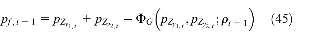
Based on Table 2, with equation (45), the structural failure probability at special time can be obtained, as shown in Table 3 and Figure 11, which can be obtained that the series-system failure probability considering the correlation between failure modes is smaller than the one without considering the correlation between failure modes. Therefore, the obtained series-system failure probability without considering the correlation between failure modes is conservative.
Structural system failure probability on special days.


Structural system failure probability on special days.
Conclusion
This article provided a new model: Gaussian copula-BDLMs, which can characterize the nonlinear correlation between failure modes and solve the reliability of the system considering nonlinear correlation between failure modes. Based on the built Gaussian copula-BDLMs, the time-dependent reliability of the series system (Yitong River Bridge main span), consisted of upper stream and lower stream middle spans, is analyzed. The results show that because there exists nonlinear correlation between the middle deflections of the upper stream and lower stream middle spans, the series-system failure probability considering the nonlinear correlation between failure modes is smaller than the one without considering the nonlinear correlation between failure modes. Therefore, it is essential and important to consider the time-dependent correlation between failure modes for obtaining the more accurate and reasonable structural system reliability.
Footnotes
Acknowledgements
The authors would like to thank the Editor and the anonymous reviewers for their constructive comments and valuable suggestions to improve the quality of the article.
Academic Editor: Xiaotun Qiu
Declaration of conflicting interests
The author(s) declared no potential conflicts of interest with respect to the research, authorship, and/or publication of this article.
Funding
The author(s) disclosed receipt of the following financial support for the research, authorship, and/or publication of this article: This work was supported by the National Natural Science Foundation of China (project no. 51608243), the Natural Science Foundation of Gansu Province of China (project no. 1606RJYA246), the Fundamental Research Funds for the Central Universities (project nos lzujbky-2015-300 and lzujbky-2015-301).