Compound Petri nets and alternatives aggregation Petri nets: Two formalisms for decision-making support

Abstract

Decision-making in technological systems, such as communication networks, manufacturing facilities and supply chains, constitutes a common requirement able to lead companies galore to success or failure. This article presents a decision-making methodology, where the feasible structural configurations to be analysed are chosen heuristically in the frame of a single optimization problem. For stating the optimization problem and solving it efficiently, appropriate formalisms would be used. Compound Petri nets, a particular kind of parametric Petri nets, and alternatives aggregation Petri nets, are two Petri net–based formalisms able to integrate in the same model different alternative structural configurations. Moreover, even having different characteristics that might make them useful for different applications, both formalisms present common features, such as including a set of exclusive entities and the possibility of developing compact Petri net models, by the removal of redundant information. This article is also focused on the transformation algorithm between compound Petri nets and alternatives aggregation Petri nets. This algorithm is devoted to transform a model described by one of the formalisms into an equivalent model, that is, with the same behaviour, represented using the other formalism. Finally, several application examples are given for illustrating the steps of the transformation algorithm.

Introduction

Decision support systems

Decision support systems constitute tools of great help to the management of systems that show complex behaviour, arisen from the interrelations between the constituent subsystems. The main topic of this article contributes to the development process of efficient decision support systems under certain assumptions.

Since the 1960s, in the 20th century, the decision support systems have been an active research field. It has focused on the information management systems based on computers, which help in the decision-making process.

The decision support systems can be found in very diverse applications including the following: (a) medical diagnosis, (b) business management, (c) airports, as well as manufacturing and (d) supply chain planning. These systems are particularly useful in environments that change swiftly.

The type of system that will be considered in this article for decision-making is the discrete event system (DES). ¹ The formal representation that has been used in this article for the DESs is the paradigm of the Petri nets (PNs).^2–5

Our civilization has experienced a significant technological development and a generalization in the use of computers in the most diverse sectors. These facts have implied that a large number of technological systems can be modelled as DESs. Among them, it can be found manufacturing systems, supply chains, and communication networks (Recalde et al., 2003). ⁶

Furthermore, the usual decisions involved in this type of systems, which have been analysed in the scientific literature include the following: (a) the design and (b) the control. In this context, control is understood as the process that allows a given system to show the desired behaviour.

For more details, the following references can be reviewed: Ramadge and Wonham, ⁷ Lee and DiCesare, ⁸ Moody and Antsaklis, ⁹ Ghaffari et al., ¹⁰ Bai et al. ¹¹ and Piera and Music. ¹²

Constraint satisfaction and optimization problems

A problem of decision-making, expressed in a formal language, might lead to the statement of a constraint satisfaction problem. This situation will happen, in case that, for solving the problem; it is enough to find a solution satisfying a given set of equalities and inequalities. On the other hand, it might be required that in addition to finding a feasible solution, it can maximize or minimize one or several quality parameters of the feasible solutions. In this case, the problem is an optimization one. ¹³

From now on, in this article, the optimization problem will be considered as the most general problem. It has to be considered that a solution of an optimization problem is one of a constraint satisfaction problem, as well. In particular, the constraint satisfaction problem is the one obtained by removing the objective or cost function from the former.

Simulation and choice of feasible solutions

A classic methodology for solving an optimization problem based on a DES consists of simulation. This methodology requires the specification of certain conditions of the model of the system, with the purpose of setting values to the unknowns associated with its controllable parameters. In this article, the term ‘undefined’ will be applied to any characteristic of the PN model or the original system, where unknowns can be found. In fact, these unknowns are associated with the freedom degrees that require a decision-making process for defining or operating the system. According to this idea, an undefined structure of a system implies that the physical constitution of the system, not necessarily its behaviour, presents freedom degrees. An undefined parameter consists of a controllable parameter of the PN model prior to a decision that specifies a value for it.

A feasible solution of the problem should be chosen, and the evolution of the system under the desired constraints should be analysed. After performing a certain number of selections and their corresponding simulations, the solution of the problem that has led to a behaviour of better quality may be the final solution for the problem. ¹⁴

Usually, the analysis of all the feasible solutions must be discarded by practical reasons. This fact can be explained because (a) the domain of the cost or objective function, also called solution space of the optimization problem, may be very large and (b) the computational cost of simulating a single solution may be also very high.

A significant limitation of simulation as optimization tool is the choice of the feasible solutions that will be considered for defining the simulation constraints.

If the selection of the feasible solutions has not been adequate and the best solutions are not chosen, the outcome of the simulation-based optimization process might not be a successful solution for the problem.

The process of searching for feasible solutions for defining the constraints of simulation can be guided, in an algorithmic procedure, by means of a probabilistic technique, such as a metaheuristic (Baruwa et al., 2015). ¹⁵ The model of the system can be represented by a type of parametric PN called compound PN, where the controllable parameters of the system are represented in a symbolic way. These parameters should be specified, as a result of the searching algorithm, by real values corresponding to the chosen solution.

Several methods can be applied for guiding the search process, such as genetic algorithms, simulated annealing, ant colony and tabu search. These algorithms explore the solution space searching for solutions that might lead to optimal values of the cost function. ¹⁶

The probabilistic nature of these methods allows escaping from local optima in their search for the global optimum. Nevertheless, metaheuristics do not guarantee that the optimum of the problem is going to be found in a given application of the methodology.

The problem of designing a new system

The DES, whose design or operation is the objective of the stated decision problem, might, in particular, present freedom degrees in its structure. This situation is very common in processes, where the system is under a process of design; hence, the lack of definition may cover many parts of the system itself. For example, there may exist a variety of alternative structural configurations for the system. Any of these structures can lead to very different models and, as a consequence, to systems of wide diversity.

This situation might arise in a design process, where different structural solutions can be taken into account. For example, it is possible to consider the design of a manufacturing system, where different suppliers may provide with different solutions for every subsystem: raw materials supply, manufacturing lines or cells, machining centres, assembly stations, quality control, reject line, storage and so on.

In this case, it is possible to build up diverse alternative solutions for the manufacturing system by means of a combination of the diverse subsystems provided by the different suppliers.

The design problem, sometimes, might produce a number of structural alternatives as a consequence of the combinatorial process arisen from the consideration of the different solutions for the subsystems. ¹⁷

The combinatorial process for constructing the feasible solutions of the decision problem may lead to a very large solution space, a situation called combinatorial explosion. This fact, in its own, justifies the requirement of particular search strategies to find promising solutions among the set of feasible solutions, impossible to explore exhaustively.

On the other hand, the structural freedom degrees can arise in other situations than in design of DESs, for example, in a control process. An example of the former is the choice in real time of a manufacturing strategy. This choice may imply changes in material and information routes, in product lot and conveying sizes and so on.

Anyway, the PN models developed for processes, where there is a diversity of alternative structural configurations, may present the following: (a) diverse sizes for the incidence matrices and (b) different values for their elements, associated with the alternative structures.

Classic solving approach: divide and conquer

A common approach for coping with the optimization of this type of systems consists of (a) selecting some of the feasible structural configurations and (b) performing simulations or specific optimization processes for each case. Following this point of view, eventually, it is possible to characterize every alternative structural configuration by a quality parameter resulting from the behaviour of the system.

In optimization problems, where there are not any undefined structural parameters, there is a single structural configuration for the system. ¹⁸ This kind of problem is a classic one, where an optimal solution can be found by means of the optimization methodology described in the following. The stages of the solution process for the optimization problems are as follows: (a) choosing a subset of promising solutions from the solution space, (b) simulating their behaviour calculating a quality parameter, (c) comparing these parameters and (d) selecting the best solution.

The classic approach to solve a similar problem with alternative structural configurations consists of the following: (a) a first step of selecting the most promising structures and (b) launching an optimization process. This process, as described in the previous paragraphs, is performed by the association of the DES with every chosen alternative structure.

Proposed solving methodology: unity makes strength

Alternatively, this article proposes a solving strategy for optimization problems with alternative structural configurations. This methodology is based on the application of the classic methodology to a case, where there is an absence of structural parameters. Instead of stating so many optimization problems as alternative structures, a single optimization process will be stated for the whole decision-making process. The possibility for doing so is based on the use of the appropriate formalisms. These proposed formalisms are included in the model itself, the complete set of alternative structural configurations: (a) compound PNs and (b) alternatives aggregation Petri nets (AAPNs).

As a first advantage of this strategy, it can be stated that it reduces the limitations in the process of intuitive selection of the structural alternatives of the system.

Furthermore, the optimization in a single process prevents the dead ends associated with the optimization processes related to specific non-successful structures. Both the proposed methodology and the classic approach often require making different types of decisions. These decisions are related not only to the structure of the system but also to other controllable non-structural parameters, such as timing and initial markings.

The main drawback of this proposed strategy is the fact that the PN model uses to be larger and more complex than a single model constructed for a unique alternative structural configuration. However, the amount of information required to describe the single PN model may be smaller than the information required to describe the set of PN models associated with different alternative structures. This reduction depends mainly in the similarity of the diverse alternative structures. The mentioned similarity is common in certain situations such as the design of DESs.^19,20

The comparison between the performance of both the proposed and the classic methodologies is favourable to the former in case there are similarities among the alternative structural configurations.

This article deals with two formalisms, based on the paradigm of the PNs. Both formalisms have been created for modelling, in a compact way, a DES with structural freedom degrees. This compactness of the model allows developing optimization procedures that, in certain cases, will be more efficient than the classic methodology.

Compound and AAPNs

The two formalisms that will be considered in this article are the compound PNs and the AAPNs. The transformation between both formalisms allows defining the equivalence conditions among models described with these different formalisms. It also allows comparing the performance of both formalisms applied to the same optimization problem. Two early versions of transformation algorithms between these two formalisms, forward and backward, were presented by Latorre-Biel and Jiménez-Macías; ²¹ however, in this article, a new, improved and complete version of the transformation algorithm, from a compound PN to an AAPN, as well as the mathematical foundations of the complete algorithm is presented and detailed.

On the other hand, the differences among both formalisms, the compound PNs and the AAPNs, can be used in diverse applications or in different stages of the same application. In this last step, it is very convenient to resort to a transformation algorithm, such as the one presented in this article. This operation might profit from one of the formalisms in a certain stage of the resolution of the decision-making problem and from the other formalism in a subsequent stage.

The structure of this article is described in this paragraph. In section ‘Modelling of a DES with an undefined structure’, several previous concepts about modelling of systems with structural undefinition, including the compound PNs and the AAPNs, will be presented. Section ‘Transformation algorithm from a compound PN to an AAPN’ is focused on the transformation algorithm to obtain an equivalent model represented by means of an AAPN, from a given model, described using the formalism of the compound PNs. Some examples to illustrate the application of this technique are presented in section ‘Examples of application’, while section ‘Application of the models to a decision-making process’ summarizes the steps for the application of the proposed decision-making process. Finally, section ‘Conclusion and future research’ deals with the conclusions and future research lines.

Modelling of a DES with an undefined structure

A compound PN is a formalism based on the paradigm of the PNs. It allows modelling a DES with an undefined structure by introducing parameters in its incidence matrices. Although an undefined PN can be defined as a PN with undefinition in any of its components (structure, marking, time, interpretation etc.), the article deals with two types of PNs with structural undefinition: compound PNs and AAPNs.

Definition 1

Compound PN. A compound PN R^c can be defined as a 7-tuple R^c = 〈P, T, Pre, Post, m₀, S_α, S_valα〉, where

1. P and T are a set of places and transitions, respectively, such that P ≠ ∅ and T ≠ ∅.

2. Pre and Post are the pre-incidence and post-incidence matrices, respectively.

3. m ₀ is the initial marking.

4. S_α = {α₁, α₂, …, α_n} is a set of controllable undefined parameters.

5. S_valα is the set of feasible combinations of values for the controllable undefined parameters. S_valα = {cv₁, cv₂, …, cv_m} verifies that the assignment (α₁, α₂, …, α_n) = cv_i should be performed as a consequence of a decision, which discards the other elements belonging to S_valα that have not been chosen.

6. |S_strα| > 1, that is to say, in order the PN to be a compound PN and not only a parametric PN, it is necessary that it includes at least a controllable undefined structural parameter.

   □

Notice that the condition 5 of the Definition 1 implies that the choice of a certain structure given by cv_strj ∈ S_valstrα = {cv_str1, cv_str2, …, cv_strm} is a consequence of a decision. Summarizing, it can be found that S_valstrα is a set of exclusive entities that reflects the nature, in turn exclusive, of the different structural alternatives for the DES with an undefined structure.

The compound PN allows to profit from the similarities or shared information among the alternative structural configurations of the DES. However, the existence of a number of undefined structural parameters, as well as of a large set of combinations of values for them, might lead the simulation of the model of the system to require a significant usage of computer resources.

In order to provide with another formalism that can be built up, without including parameters in the incidence matrices, by means of different modelling procedures, the AAPNs have been created. The AAPNs present a conceptual proximity with the coloured PNs.

The first element of an AAPN bears the exclusive nature of the structural alternatives modelled by the net.

Definition 2. Choice variables

A set of choice variables is defined in the following way

$$\begin{array}{cc}\multicolumn{1}{c}{S_A=}& \{a_1,a_2,\dots ,a_s|\exists !a_i=1,\mathrm{where}i\in N^{*},\hfill \\ \multicolumn{1}{c}{}& 1\le i\le s\wedge a_j=0\forall j\ne i,1\le j\le s\}\hfill \end{array}$$

Moreover, the assignment a_i = 1 is the result of a decision.

□

As a consequence, the role that S_valstrα plays in a compound PN, in the case of an AAPN is carried out by S_A.

Definition 3. AAPN

An AAPN, R^A, can be defined as the following 9-tuple

$$R^A=〈P,T,\mathrm{Pre},\mathrm{Post},{\mathbf{m}}_0,S_{\alpha },\mathrm{Sva}{l}_{\alpha },S_A,f_A〉$$

where

1. P and T are a set of places and transitions, respectively, which verify P ≠ ∅ and T ≠ ∅.

2. Pre and Post are the pre-incidence and post-incidence matrices, respectively.

3. m ₀ is the initial marking.

4. S_α = {α₁, α₂, …, α_n} is a set of controllable undefined parameters. In an AAPN, it might happen that S_strα = ∅.

5. S_valα is the set of feasible combinations of values for the controllable undefined parameters.

6. S_A is a set of choice variables, such that |S_A| > 1.

7. f_A: T → f(a₁, …, a_n) is a function that assigns to every transition t a Boolean function of choice variables.

   □

In the previous definition, the role played by f_A guarantees that every choice variable can be associated with a set of transitions. This choice variable would be evaluated before the evolution of the system begins, once that a decision has allowed activating one of the choice variables.

It is interesting to consider that the set of undefined structural parameters of R^A is a subset of the undefined parameters: S_strα ⊆ S_α. If S_strα = ∅, then R^A is called a simple AAPN, while in case that S_strα ≠ ∅, then R^A is a compound AAPN.

As a consequence of the previous considerations, it can be seen that the evolution rules for an AAPN change slightly from the dynamics of a generalized PN.

In particular, before the AAPN begins its evolution, a decision must be made concerning which choice variable should be activated. This decision assigns ‘0’, meaning not chosen, to all the other choice variables.

Definition 4. Enabled transition of an AAPN

Let us consider an AAPN R^A associated with a set of choice variables S_A = {a₁, a₂, …, a_s}; let us consider the following decision

$$a_i=1\Rightarrow a_i=0\forall j\in N^{*}\mathrm{such}\mathrm{that}1\le j\le n\wedge j\ne i$$

A certain transition t_j ∈ T of an AAPN is said to be enabled if

$$m_i\ge \mathrm{Pre}(p_i,t_j)\forall p_i\in \circ t_j\wedge f_A\left(t_j\right)=1$$

□

In other words, transition t_j belonging to the PNs enabled when the number of tokens in place p_i is at least as large as the weight of the arc connecting p_i with t_j, for every place p_i which are input places to the transition t_j, and the function of choice variables associated with this transition leads to a true value if evaluated.

It should be noticed that it is not necessary to evaluate f_A(t_j) in every step of the evolution of the AAPN. It is possible to evaluate every function of choice variables associated with the transitions before starting the simulation and to remove every transition associated with a function of choice variables with value False.

On the other hand, the transitions that are associated with a function of choice variables, whose value is True, should be preserved, but the function can be removed.

Transformation algorithm from a compound PN to an AAPN

Let us consider the following compound PN R^c = 〈P, T, Pre, Post, m₀, S_α, S_valα〉:

• Step 1. Define a set of choice variables from S_valstrα(R^c) = {cv_str1, cv_str2, …, cv_strm} in the form S_A = {a₁, a₂, …, a_m| ∃! a_i = 1, 1 ≤ i ≤ m, a_j = 0 ∀ j ≠ i, 1 ≤ j ≤ m}, where |S_A| = |S_valstrα(R^c)| = m.

• Step 2. Create a bijection among the elements of S_valstrα(R^c) and the choice variables of S_A.

• Step 3. Replicate every transition t_i in the set $\{t_i^1,t_i^2,\dots ,t_i^m\}$ , where m = |S_A| and

• The choice variable a_q is associated with the transition $t_i^q$ as a Boolean condition for controlling the enabling of the transition.

Step 4. Transform the AAPN resulting from the application of step 3 removing the isolated transitions and places.

Step 5. Application of a reduction rule to quasi-identical transitions, associated with different choice variables, thus obtaining an AAPN with a reduced set of transitions.

□

The step 5 of the previous algorithm requires to define the concept of quasi-identical transitions, see Figure 1, and to formulate the reduction rule.

Figure 1.

Subnet associated with the set of quasi-identical transitions t₁, t₂, …, t_n.

Definition 5. Quasi-identical transition

Let t₁, t₂, …, t_n ∈ T(R^A) be a set of transitions of an AAPN. A pair of transitions belonging to T(R^A) is said to be quasi-identical if they verify the following properties:

1. ∀t_i, t_j ∈ T(R^A) ∃ a_i, a_j ∈ S_A such that a_i is associated with t_i, and a_j is associated with t_j, where t_j ≠ t_j.

2. ∀t_i, t_j ∈ T(R^A) if it is removed the association with a_i and a_j ⇒ t_i and t_j are identical transitions. ²²

   □

Proposition. Reduction rule for quasi-identical transitions

Let R^A be an AAPN and S_A its associated set of choice variables.

Let t₁, t₂, …, t_n ∈ T(R^A) be n quasi-identical transitions of the AAPN, such that ∀t_i ∈ T(R^A), where 1 ≤ i ≤ n, a_i is associated with t_i, with a_i ∈ S_A (see Figure 1).

Let t be, without associated choice variables, an identical transition to t₁, t₂, …, t_n. If the function of choice variables a₁ + a₂ + ··· + a_n, where + is the logic operator ‘OR’, is associated with t, then it is possible to state that t is equivalent to t₁, t₂, …, t_n.

Proof

In order to analyse the behaviour of both equivalent subnets, one related to transition t, see Figure 2, and other associated with the set of quasi-identical transitions t₁, t₂, …, t_n, see Figure 1, it is necessary, first of all, to select arbitrarily one of the choice variables to be activated. As a result of this selection, the choice variable a_q ∈ S_A will be activated, with 1 ≤ q ≤ n.

Figure 2.

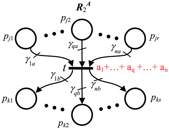
Subnet associated with the transition t.

By definition of choice variables, the rest of the choice variables a_i ∈ S_A, i ≠ q, 1 ≤ i ≤ n, will verify that a_i = 0.

This fact implies that in the evolution of the AAPNs, where the set of identical transitions t₁, t₂, …, t_n exists, only t_q can be enabled, hence, the rest of them can be removed (see Figure 3).

Figure 3.

Subnet associated with the set of choice variables t₁, t₂, …, t_n after the activation of the choice variable a_q.

On the other hand, the function of choice variables a₁ + a₂ + ··· + a_n associated with t will verify that a₁ + a₂ + ··· + a_n = 0 + ··· + 0 + a_q + 0 + ··· + 0 = 1 (see Figure 4).

Figure 4.

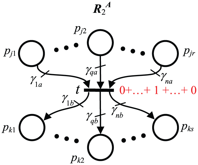
Subnet associated with the transition t after the activation of the choice variable a_q.

Due to the fact that t and t_q are identical transitions, and they are both associated with an activated choice variable or function of choice variables, their behaviour is the same. This reasoning can be repeated for any of the other transitions of the set t₁, t₂, …, t_n with the same results. As a consequence, t₁, t₂, …, t_n and t are equivalent.

Examples of application

Example 1

Let us consider the compound PN depicted in Figure 5.

Figure 5.

Compound Petri net.

In this first example, a compound PN will be transformed into an equivalent AAPN by means of the application of the steps of the algorithm described in the previous section.

The set of undefined parameters of the original compound PN contains only five structural parameters S_α(R^c) = S_strα(R^c) = {α₁, α₂, α₃, α₄, α₅}. On the other hand, the set of feasible combinations of values for the undefined structural parameters has three elements: S_valstrα(R^c) = {(0,2,0,0,0), (0,1,1,1,0), (1,2,0,1,2)}:

• Step 1. S_valstrα(R^c) = {(0,2,0,0,0), (0,1,1,1,0), (1,2,0,1,2)}, |S_valstrα(R^c)| = 3 = |S_A|.

Hence, it is possible to create the following set of choice variables

$$\begin{array}{c}{S}_A=\{a_1,a_2,a_3|\exists !a_i=1,\hfill \\ 1\le i\le 3,a_j=0\forall j\ne i,1\le j\le 3\}\hfill \end{array}$$

• Step 2. Create a bijection between the elements of S_valstrα(R^c) and S_A (see Figure 6).

• Step 3. Replicate every transition t_i in the set $\{t_i^1,t_i^2,\dots ,t_i^m\}$ , where 3 = |S_A| and 1 ≤ i ≤ 3.

Figure 6.

Bijection between S_A and S_valstrα(R^c).

In order to calculate the weight of the arcs of every replicated transitions, the structural parameters associated with every cv_strq ∈ S_valstrα(R^c) = {cv_str1, cv_str2, …, cv_strm} with 1 ≤ q ≤ 3 will be considered. On the other hand

$$\begin{array}{c}{S_{\mathrm{str}}}_a=\left\{(a_1,a_2,a_3,a_4,a_5)\right\}\hfill \\ c{v_{\mathrm{str}}}_1=(0,2,0,0,0),\hfill \\ c{v_{\mathrm{str}}}_2=(0,1,1,1,0),c{v_{\mathrm{str}}}_3=(1,2,0,1,2)\hfill \end{array}$$

The values of the defined structural parameters defined of R^c are given by the following expression (see Figure 7)

$$\begin{array}{l}{S}_{strb}=\{({\beta }_6,{\beta }_7,{\beta }_8,{\beta }_9)\},\\ \mathrm{where}({\beta }_6,{\beta }_7,{\beta }_8,{\beta }_9)=\left(1,1,1,0\right)\end{array}$$

Figure 7.

Naming of the structural parameters of R^c.

Transition t₁ is replicated in $\{t_1^1,t_1^2,t_1^3\}$ . In this case, i = 1

$$\begin{array}{cc}\multicolumn{1}{c}{q}& =1\Rightarrow (v_q^1,v_q^2,\dots ,v_q^m)\hfill \\ \multicolumn{1}{c}{}& =({\alpha }_1,{\alpha }_2,{\alpha }_3,{\alpha }_4,{\alpha }_5,{\beta }_6,{\beta }_7,{\beta }_8,{\beta }_9)\hfill \\ \multicolumn{1}{c}{}& =(0,2,0,0,0,1,1,1,0)\hfill \\ \multicolumn{1}{c}{}& j=1\Rightarrow \mathrm{Pre}(p_j,t_i^q)=\mathrm{Pre}(p_1,t_1^1)={\beta }_6=1\hfill \\ \multicolumn{1}{c}{}& k=2\Rightarrow \mathrm{Post}(t_i^q,p_k)=\mathrm{Post}(t_1^1,p_2)={\alpha }_2=2\hfill \\ \multicolumn{1}{c}{}& k=3\Rightarrow \mathrm{Post}(t_i^q,p_k)=\mathrm{Post}(t_1^1,p_3)={\alpha }_3=0\hfill \end{array}$$

$$\begin{array}{cc}\multicolumn{1}{c}{q}& =2\Rightarrow (v_q^1,v_q^2,\dots ,v_q^m)\hfill \\ \multicolumn{1}{c}{}& =({\alpha }_1,{\alpha }_2,{\alpha }_3,{\alpha }_4,{\alpha }_5,{\beta }_6,{\beta }_7,{\beta }_8,{\beta }_9)\hfill \\ \multicolumn{1}{c}{}& =(0,1,1,1,0,1,1,1,0)\hfill \\ \multicolumn{1}{c}{}& j=1\Rightarrow \mathrm{Pre}(p_j,t_i^q)=\mathrm{Pre}(p_1,t_1^2)={\beta }_6=1\hfill \\ \multicolumn{1}{c}{}& k=2\Rightarrow \mathrm{Post}(t_i^q,p_k)=\mathrm{Post}(t_1^2,p_2)={\alpha }_2=1\hfill \\ \multicolumn{1}{c}{}& k=3\Rightarrow \mathrm{Post}(t_i^q,p_k)=\mathrm{Post}(t_1^2,p_3)={\alpha }_3=1\hfill \end{array}$$

$$\begin{array}{cc}\multicolumn{1}{c}{q}& =3\Rightarrow (v_q^1,v_q^2,\dots ,v_q^m)\hfill \\ \multicolumn{1}{c}{}& =({\alpha }_1,{\alpha }_2,{\alpha }_3,{\alpha }_4,{\alpha }_5,{\beta }_6,{\beta }_7,{\beta }_8,{\beta }_9)\hfill \\ \multicolumn{1}{c}{}& =(1,2,0,1,2,1,1,1,0)\hfill \\ \multicolumn{1}{c}{}& j=1\Rightarrow \mathrm{Pre}(p_j,t_i^q)=\mathrm{Pre}(p_1,t_1^3)={\beta }_6=1\hfill \\ \multicolumn{1}{c}{}& k=2\Rightarrow \mathrm{Post}(t_i^q,p_k)=\mathrm{Post}(t_1^3,p_2)={\alpha }_2=2\hfill \\ \multicolumn{1}{c}{}& k=3\Rightarrow \mathrm{Post}(t_i^q,p_k)=\mathrm{Post}(t_1^3,p_3)={\alpha }_3=0\hfill \end{array}$$

The process is repeated with the replication of transition t₂ $\{t_2^1,t_2^2,t_2^3\}$ and t₃ in $\{t_3^1,t_3^2,t_3^3\}$ :

• 2. As a second stage in the step 3 of the transformation algorithm, the choice variable a_q is associated with the transition $t_i^q$ as a Boolean condition that controls the enabling of the transition 1 ≤ i ≤ 3.

The result of step 3 of the algorithm, consisting of the replication of every transition, can be seen in Figure 8.

Figure 8.

Graphical representation of R^c after replicating the transitions.

It can be seen in the resulting AAPNs that it lacks undefined structural parameters in contrast with the original compound PN.

Furthermore, the association of the choice variables with the replicated transitions models the exclusiveness of the different alternative structural configurations. This exclusiveness requires making a decision before the evolution of the PN begins:

• Step 4. Removal of the isolated places and transitions.

The isolated places and transitions lack of arc connecting them to other nodes of the net. For this reason, they do not intervene in the flow of tokens that describes the evolution of the system. As a consequence, the isolated places and transitions can be removed from the AAPN without altering its behaviour.

The first stage of step 4 consists of identifying and removing from the AAPN all the arcs with weight zero. The result can be seen in Figure 9.

Figure 9.

Alternatives aggregation Petri nets after removing the zero-weighted arcs.

As a next step of step 4, the isolated places and transitions should be identified and removed. In this example, there are two isolated transitions: $t_3^1$ and $t_3^2$ . In order to conclude step 4, the isolated transitions should be removed. The result can be seen in Figure 10.

Figure 10.

Alternatives aggregation Petri net after the application of step 4.

• Step 5. Apply the reduction rule to the quasi-identical transitions, obtaining an AAPN with a reduced set of transitions.

In the reduction rule for quasi-identical transitions, it can be seen that a set of quasi-identical transitions can be reduced to a single transition associated with a certain function of choice variables.

In order to find quasi-identical transitions, it is necessary to search for identical transitions in the generalized PN obtained by removing the choice variables of the AAPN.

In the identical transitions, the input and output arcs should connect the transitions with the same places and should be weighted with the same values. On a further step, it should be checked whether the associated choice variables verify the condition of the reduction rule.

In the present example, two pairs of quasi-identical transitions have been found: $t_1^1$ and $t_1^3$ on one side and $t_2^2$ and $t_2^3$ on the other. The application of the reduction rule allows the substitution of the first pair for the transition $t_r^1$ , which is associated with the function of choice variables a₁ + a₃. Moreover, the second pair of quasi-identical transitions can be replaced by $t_r^2$ , associated with the function a₂ + a₃. The result of this last step of the algorithm is depicted in Figure 11.

Figure 11.

Alternatives aggregation Petri net, equivalent to the compound Petri net R^c.

Example 2

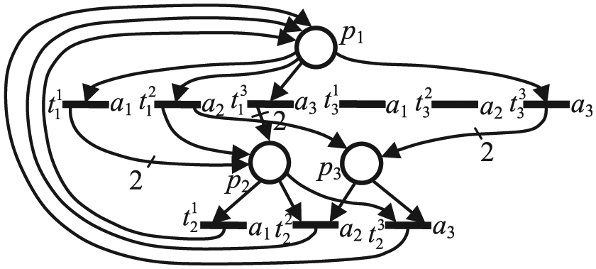
In the following, a compound PN in both representations can be seen: a graphical one in Figure 12 and another matrix-based one based on the incidence matrix in Figure 13.

Figure 12.

Compound PN.

Figure 13.

Matrix-based representation of the compound Petri net.

The set of structural parameters of the compound PN R^c is as follows

$$\begin{array}{c}{S_{\mathrm{str}}}_{\gamma }\left(R^c\right)=\{{\alpha }_1,{\beta }_2,{\beta }_3,{\alpha }_4,{\alpha }_5,{\beta }_6\}\hfill \\ ={S_{\mathrm{str}}}_{\alpha }\left(R^c\right)\cup {S_{\mathrm{str}}}_{\beta }\left(R^c\right),\mathrm{where}\hfill \\ ={S_{\mathrm{str}}}_{\alpha }\left(R^c\right)=\{{\alpha }_1,{\alpha }_4,{\alpha }_5\}\mathrm{and}{S_{\mathrm{str}}}_{\beta }\left(R^c\right)\hfill \\ =\{{\beta }_2,{\beta }_3,{\beta }_6\}\hfill \end{array}$$

On the other hand, the set of feasible values for the structural parameters of R^c can be written as follows

$$\begin{array}{c}{S_{\mathrm{valstr}}}_{\beta }\left(R^c\right)=\left\{(1,1,1)\right\}\hfill \\ {S_{\mathrm{valstr}}}_{\alpha }\left(R^c\right)=\{(1,0,1),(0,1,0),(2,0,1),(0,1,2)\}\hfill \end{array}$$

Finally, it is possible to determine the set of feasible values for every undefined structural parameter of R^c

$$\begin{array}{c}{S}_{\mathrm{val}\alpha 1}\left(R^c\right)=\{0,1,2\}\hfill \\ S_{\mathrm{val}\alpha 4}\left(R^c\right)=\{0,1\}\hfill \\ S_{\mathrm{val}\alpha 5}\left(R^c\right)=\{0,1,2\}\hfill \end{array}$$

The first partition of S_valstrα(R^c) has order 2 and can be represented as follows

$$\begin{array}{c}\underset{1}{\Pi }\left({S_{\mathrm{valstr}}}_{\alpha }\left(R^c\right)\right)=\{{S_{1\mathrm{valstr}}}_{\alpha }\left(R^c\right),{S_{2\mathrm{valstr}}}_{\alpha }\left(R^c\right)\}\hfill \\ {S_{\mathrm{valstr}}}_{\alpha }\left(R^c\right)={S_{1\mathrm{valstr}}}_{\alpha }\left(R^c\right)\cup {S_{2\mathrm{valstr}}}_{\alpha }\left(R^c\right)\hfill \\ {S_{\mathrm{valstr}}}_{\alpha }\left(R^c\right)=\{(1,0,1),(0,1,0),(2,0,1),(0,1,2)\}\hfill \\ {S_{1\mathrm{valstr}}}_{\alpha }\left(R^c\right)=\{(1,0,1),(0,1,0)\}\hfill \\ {S_{2\mathrm{valstr}}}_{\alpha }\left(R^c\right)=\{(2,0,1),(0,1,2)\}\hfill \end{array}$$

In order to know the number of undefined structural parameters associated with every subset of the partition, it is necessary to analyse every parameter of S_valstrα(R^c).

On one hand, the first subset of the partition will be considered

$$\begin{array}{c}{S}_{1\mathrm{val}{\alpha }_1}\left(R^c\right)=\{0,1\}\hfill \\ S_{1\mathrm{val}{\alpha }_4}\left(R^c\right)=\{0,1\}\hfill \\ S_{1\mathrm{val}{\alpha }_5}\left(R^c\right)=\{0,1\}\hfill \end{array}$$

As a consequence, there will be three undefined structural parameters associated with this subset of the partition, since any of them can take values from a set with more than one element

$${S_{1\mathrm{str}}}_{\alpha }\left(R^c\right)=\{{\alpha }_1^1,{\alpha }_4^1,{\alpha }_5^1\}$$

On the other hand, the second subset of the partition will lead to the following

$$\begin{array}{c}{S}_{2\mathrm{val}{\alpha }_1}\left(R^c\right)=\{0,2\}\hfill \\ S_{2\mathrm{val}{\alpha }_4}\left(R^c\right)=\{0,1\}\hfill \\ S_{2\mathrm{val}{\alpha }_5}\left(R^c\right)=\{1,2\}\hfill \end{array}$$

In this case, there will be another new three undefined structural parameters associated with this subset of the partition, since any of them can take values from a set with more than one element

$${S_{2\mathrm{val}}}_{\alpha }\left(R^c\right)=\{{\alpha }_1^2,{\alpha }_4^2,{\alpha }_5^2\}$$

As a result, it is possible to see how this partition of S_valstrα(R^c), Π₁(S_valstrα(R^c)), from a compound PN with three undefined structural parameters leads to a representation with six undefined structural parameters. This representation can be a set of compound alternative PN or an AAPN. The AAPN that results from the replication of the transitions of the compound PN R^c according to this partition is represented in Figure 14(a) and its incidence matrix is shown in Figure 14(b).

Figure 14.

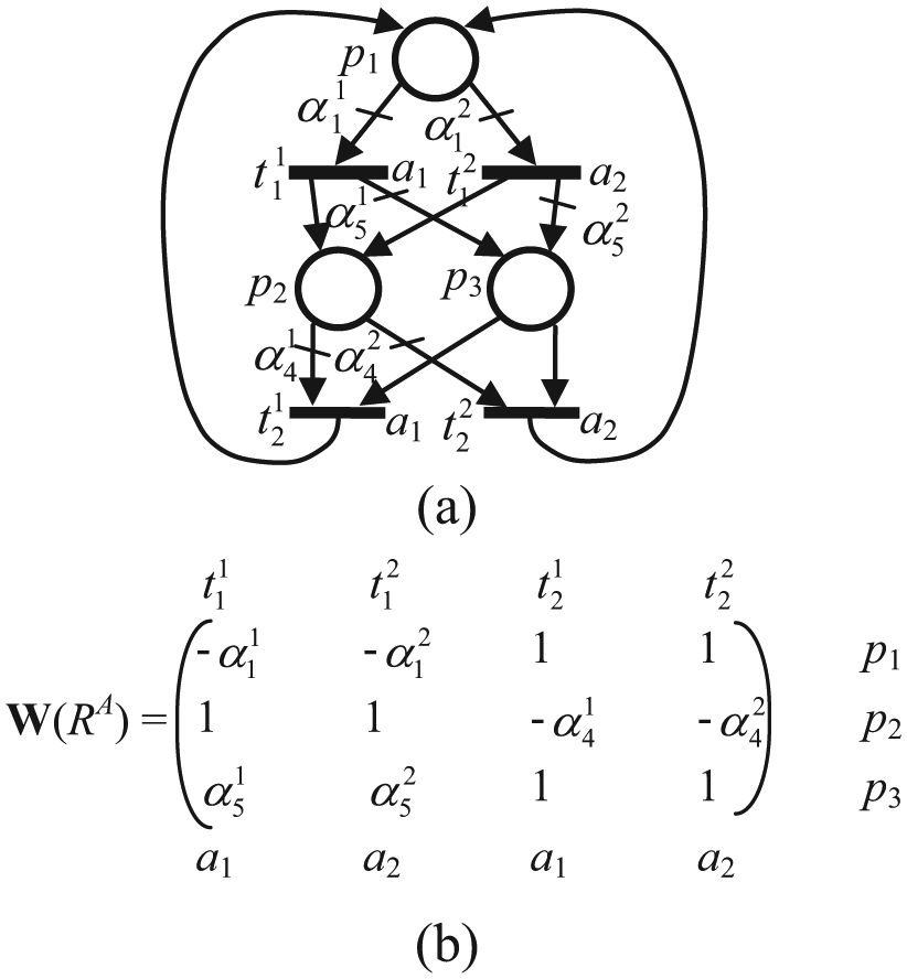
Graphical representation of an alternatives aggregation Petri net: (a) obtained from first partition of S_valstrα(R^c) and (b) matrix-based representation obtained from a first partition of S_valstrα(R^c).

As a conclusion, it is possible to state that despite the fact that the original compound PN R^c has only three undefined structural parameters S_strα(R^c) ={α₁, α₄, α₅}, the resulting AAPN obtained by a replication of the transitions based on this first partition of S_valstrα(R^c) has six undefined structural parameters

$${S_{\mathrm{str}}}_{\alpha }\left(R^A\right)={S_{1\mathrm{str}}}_{\alpha }\left(R^c\right)\cup {S_{2\mathrm{str}}}_{\alpha }\left(R^c\right)=\{{\alpha }_1^1,{\alpha }_1^2,{\alpha }_4^1,{\alpha }_4^2,{\alpha }_5^1,{\alpha }_5^2\}$$

Example 3

The second partition of S_valstrα(R^c) has order 2 and can be represented as follows

$$\begin{array}{c}\underset{2}{\Pi }\left({S_{\mathrm{valstr}}}_{\alpha }\left(R^c\right)\right)=\{{S_{1\mathrm{valstr}}}_{\alpha }\left(R^c\right),{S_{2\mathrm{valstr}}}_{\alpha }\left(R^c\right)\}\hfill \\ {S_{\mathrm{valstr}}}_{\alpha }\left(R^c\right)={S_{1\mathrm{valstr}}}_{\alpha }\left(R^c\right)\cup {S_{2\mathrm{valstr}}}_{\alpha }\left(R^c\right)\hfill \\ {S_{\mathrm{valstr}}}_{\alpha }\left(R^c\right)=\{(1,0,1),(0,1,0),(2,0,1),(0,1,2)\}\hfill \\ {S_{1\mathrm{valstr}}}_{\alpha }\left(R^c\right)=\{(1,0,1),(2,0,1)\}\hfill \\ {S_{2\mathrm{valstr}}}_{\alpha }\left(R^c\right)=\{(0,1,0),(0,1,2)\}\hfill \end{array}$$

In order to know the number of undefined structural parameters associated with every subset of the partition, it is necessary to analyse every parameter of S_valstrα(R^c).

On one hand, the first subset of the partition will be considered

• S _1valα1(R^c) = {1, 2}

• S _1valα4(R^c) = {0} ⇒ In this subset of the second partition, α₄ is no longer an undefined structural parameter but a defined one: ${\beta }_4^1$ .

• S _1valα5(R^c) = {1} ⇒ In this subset of the second partition, α₅ is no longer an undefined structural parameter but a defined one: ${\beta }_5^1$ .

As a consequence, there will be only one undefined structural parameter associated with this subset of the partition, since only ${\alpha }_1^1$ can take values from a set with more than one element

$$S_{1\mathrm{val}{\alpha }_1}\left(R^c\right)=\left\{{\alpha }_1^1\right\}$$

On the other hand, the second subset of the partition will lead to the following:

• S _2valα1(R^c) = {0} ⇒ In this subset of the second partition, α₁ is no longer an undefined structural parameter but a defined one: ${\beta }_1^1$ .

• S _2valα4(R^c) = {1} ⇒ In this subset of the second partition, α₄ is no longer an undefined structural parameter but a defined one: ${\beta }_4^1$

• S _2valα5(R^c) = {0, 2}

This case will provide with another single undefined structural parameter associated with the corresponding subset of this second partition, ${\alpha }_5^2$ , since it is the only one that can take values from a set with more than one element

$${S_{2\mathrm{val}}}_{\alpha }\left(R^c\right)=\left\{{\alpha }_5^2\right\}$$

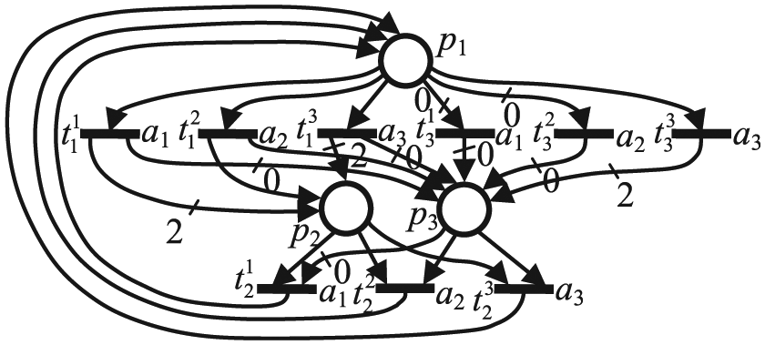
As a result, it is possible to see how this second partition of S_valstrα(R^c), Π₂(S_valstrα(R^c)), from a compound PN with three undefined structural parameters leads to a representation with only two undefined structural parameters. This representation can be a set of compound alternative PN or an AAPN. The AAPN that results from the replication of the transitions of the compound PN R^c according to this partition is represented in Figures 15 and 16.

Figure 15.

Graphical representation of an alternatives aggregation Petri net obtained from a second partition of S_valstrα(R^c).

Figure 16.

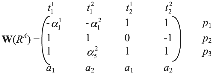
Matrix-based representation of an alternatives aggregation Petri net obtained from a second partition of S_valstrα(R^c).

As a conclusion, it is possible to state that despite the fact that the original compound PN R^c has only three undefined structural parameters S_strα(R^c) ={α₁, α₄, α₅}, the resulting AAPN obtained by a replication of the transitions based on this second partition of S_valstrα(R^c) has only two undefined structural parameters

$${S_{\mathrm{str}}}_{\alpha }\left(R^A\right)={S_{1\mathrm{str}}}_{\alpha }\left(R^c\right)\cup {S_{2\mathrm{str}}}_{\alpha }\left(R^c\right)=\{{\alpha }_1^1,{\alpha }_5^2\}$$

It is interesting to notice that it depends on the parameters of the transformation algorithm (in this case the chosen partition) that the size of the resulting model is more or less compact.

Application of the models to a decision-making process

The process of decision-making associated with the previous examples might be carried out in the following way:

• Step 1. Define the optimization problem to be solved:

• Step 1.2. Determine a quantitative method for assessing the quality of a given solution. For example, define a cost function.

• Step 1.3. Determine the additional constraints of the decision problem. For instance, the time period of the PN and the model of a dynamic DES that covers the statement of the problem.

Step 2. Define the search method for feasible solutions in the solution space. For example, a metaheuristic, such as genetic algorithms, tabu search, swarm particle, ant colony or simulated annealing.

Step 3. Launch an instance of the optimization problem:

Step 3.1. Select one feasible solution using the search algorithm.

Step 3.2. Simulate the behaviour of the PN model of the system under the chosen solution and the constraints of the problem.

Step 3.3. Calculate the quality of the simulated solution.

Step 3.4. If it is the first solution analysed, store it, otherwise, compare the quality of the new solution with the one of the stored solution and store the best of them.

Step 3.5. Evaluate the stopping criterion for deciding if a new solution should be evaluated (step 3.1) or the process is terminated. The solution of the optimization problem given by this technique is the best solution found by the algorithm.

This algorithm does not guarantee that the solution found is the optimum of the stated optimization problem. However, it is likely to be close to it; for this reason, it can be called quasi-optimal solution. The quality of this quasi-optimal solution will depend on the tuning of the search algorithm, as well as on the computational resources and time devoted to solve the problem.

Conclusion and future research

In this article, it has been shown how it is possible to relate two formalisms that have been created for representing a DES with an undefined structure, by means of a transformation algorithm. Both formalisms, based on the paradigm of the PN, the compound PNs and the AAPNs share the possibility of removing redundant information in models built up from alternative PNs.

Nevertheless, the compactness of the model in the case of the AAPNs is achieved by means of sets of structural parameters and the feasible combination for their values. On the other hand, the capacity for condensing information, in the case of the AAPNs, is based on the existence of shared subnets and the possibility of controlling the token flow in the evolution of the PN by means of the choice variables.

Both formalisms, compound PNs and AAPNs, have led to promising results while implementing optimization algorithms with guided search by means of metaheuristics based on genetic algorithms.

However, there is a long way ahead in applying the methodology described in this article, in a variety of real cases, which will allow acquiring knowledge on the practical advantages and drawbacks of any of the presented formalisms.