Sage Journals: Discover world-class research

Abstract

Degradation failure is one of the main reasons for complex mechanical systems losing their functions. Research on multidisciplinary design optimization under uncertainties should shift from static uncertainties to time-varying uncertainties. Aiming at time-varying uncertainties in mechanical systems, we put forward a multidisciplinary reliability design optimization method using stochastic process theory. First, we investigated the characteristics of time-varying uncertainties in complex mechanical systems, and then utilized stochastic process theory to quantify time-varying uncertainties. Second, through combining the multidisciplinary simultaneous analysis and design optimization method, the model of multidisciplinary design optimization under time-varying uncertainties is established. Moreover, a mathematical problem and an engineering example are provided to illustrate the accuracy and effectiveness of the proposed method.

Keywords

Multidisciplinary design optimization time-varying uncertainty stochastic process time-varying reliability model simultaneous analysis and design

Introduction

Multidisciplinary design optimization (MDO) of complex mechanical systems has shown wide application recently.^1–4 Increasing attentions are being paid on MDO under uncertainties in recent years. Du and Chen^5,6 proposed an uncertainty calculation method based on global and local sensitivity equation by combining uncertainty analysis method with error propagation in the process of physical measurement, and then put forward a system uncertainty analysis (SUA) method and concurrent subsystem uncertainty analysis (CSSUA) method. Gu et al.⁷ derived limit expression of uncertainty propagation based on Taylor series method, and then built stochastic uncertainty analysis model. The above-mentioned researches have made tremendous contributions on MDO under aleatory and epistemic uncertainties. However, note from researches in previous studies^8–13 that the degradation failure is one of the main reasons for complex mechanical systems lost their functions. There are variant time-varying uncertainties in complex mechanical systems, such as performance degradation of electronic component, strength decrease, material aging, wear, oxidation, and corrosion.^14,15 Although research methods to deal with aleatory and epistemic uncertainties in MDO may largely improve the reliability of complex systems, however, these research methods cannot accurately describe the sources, essential characteristics, and propagation properties of time-varying uncertainties and cannot simply be applied to deal with time-varying uncertainties in MDO.

Currently, methods to deal with time-varying uncertainties under single-discipline analysis can be divided into two categories. (1) Probabilistic reliability methods, such as Bayesian method and Monte Carlo method. These methods are very effective when dealing with random time-varying uncertainties. However, these methods need to know the probability distributions in advance, require that time is clearly defined, and samples must be adequate. In addition, these prerequisites are often difficult to obtain in the design process. Melchers¹⁶ indicate that when there is only one random load, the force can be expressed by the extreme value distribution, and then calculate structure failure probability using either first order reliability method (FORM) or second order reliability method (SORM) method, another case is that using series reliability method to calculate the reliability of the life cycle by only considering some of the key period in life cycle, such as storm periods. Veneziano et al.¹⁷ assumed that time-varying uncertainties are Gauss distributions and proposed a system reliability analysis method. Breitung and Rackwitz¹⁸ proposed a system reliability analysis method using rectangular wave renewal process to describe time-varying uncertainties, and combined Gauss process and rectangular wave renewal process to deal with time-varying uncertainties.^19–21 Li and Zhang²² assumed that the deterioration process of resistance was a Gamma process and proposed a time-variant reliability assessment. (2) Non-probabilistic reliability methods, such as interval analysis and convex sets. These methods do not take full advantage of the information in design process and the final design results are conservative. According to the upper and lower boundary of time-interval reliability, Shinozuka²³ provided calculation formulas. Andrieu-Renaud et al.,²⁴ Cazuguel et al.,²⁵ and Li and Mourelatos²⁶ established the formulas to calculate the time-varying reliability index and compared the differences and relations between time interval reliability and moment reliability. Jiang et al.²⁷ proposed an effective non-probabilistic model process method for time-variant uncertainty analysis.

Until now, the methods to process time-varying uncertainties under single-discipline analysis have made certain progress. However, during the whole product life cycle, forms of time-varying uncertainties are diversified and often correlated to each other. Since there are hierarchical and non-hierarchical hybrid coupled relationships between subsystems in MDO, time-varying uncertainties which exist in subsystem levels may have different influence on the final output of the system. In addition, MDO is a kind of coordination system optimization method for large systems, which leads to difficulties to quantify time-varying uncertainties.

Aiming at dealing with time-varying uncertainties in MDO, this article proposes a multidisciplinary reliability design optimization (MRDO) method under time-varying uncertainties. The remainder of this article is arranged as follows. In section “Time-varying reliability model,” we analyze the characteristics of time-varying uncertainties, and then introduce stochastic Ito process to quantify time-varying uncertainties. In section “Time-varying reliability MDO,” MDO model under time-varying uncertainties is established, and the specific operation steps are given. In section “Case studies,” a mathematical problem and an engineering example are given to illustrate the feasibility and effectiveness of the proposed method. Section “Conclusion” gives the research conclusion.

Time-varying reliability model

Reliability analysis under time-varying uncertainties

For mechanical products, time-varying uncertainties include material performance, working environment, service time, and load effect.^14,15 The product performance degrades gradually over time. The degradation process of product performance is a dynamic time-varying process.¹⁵ Time-varying reliability method is often applied to deal with time-varying uncertainties. Time-varying reliability means that the failure rate p_f (t₀–t₁) of limit state function is less than the given failure rate during time interval t₀–t₁. In other words, the reliability R of limit state function at any time is greater than the allowable reliability [R], which is shown in Figure 1.

Figure 1.

Time-varying reliability diagram.

Currently, the methods considering time-varying uncertainties assume that strength and stress of mechanical parts follow certain probability distributions, respectively,^28–31 which cannot be used to evaluate dynamic evolution process of time-varying uncertainties. According to this, we attempt to propose a time-varying reliability prediction model based on stochastic differential equation theory which can calculate the reliability index at any time.

Stochastic differential equation

Compared to traditional probability methods, Ito differential equation is better to deal with uncertainties in mechanical systems. The structure of Ito differential equation is simple, theoretical concept is clear, so it is very easy to combine Ito differential equation with MDO to solve time-varying uncertainties. Assume Ω = {ω} is the sample space of stochastic experiment, and T is a set of parameters (time). For each t∈T, there is a random variable X(t, ω). A set of variables X(t, ω) is a stochastic process. The definition domain of ω is the entire sample space, and the definition domain of t is the entire timeline [0, ∞] or a time period [0, T]³²

X (t, ω) : {Ω} \times [0, T] \to R

Assume that there are m time-varying factors, then

X (t, ω) = [x_{1} (t, ω), x_{2} (t, ω), \dots, x_{m} (t, ω)]^{T}

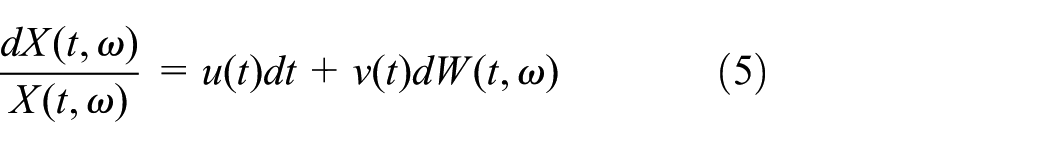
Set (Ω, F, P) is a probability space; F is the σ-algebra of Ω, P is the probability measure of Ω, and the random variable X(t, ω) should satisfy the following Ito equation

{\begin{matrix} dX (t, ω) = u (t) X (t, ω) dt + v (t) X (t, ω) dW (t, ω) \\ X (t_{0}) = X_{0} \end{matrix}

(1)

where u(t) is the drift rate which reflects the influence of deterministic factors, and v(t) is the fluctuation rate which reflects the influence of time-varying uncertainties.

The drift rate can be expressed as follows

u (t) = \frac{1}{n - 1} \sum_{1}^{n} \ln \frac{X_{i + 1}}{X_{i}}

(2)

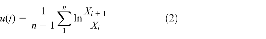
where X_i is the observation value at time point i (i = 1, 2, …, n).

The fluctuation rate can be expressed as

v (t) = {[\sum_{1}^{n} \frac{{(\ln \frac{X_{j + 1}}{X_{j}} - u (t))}^{2}}{n - 1}]}^{1 / 2}

(3)

where X_j is the observation at time point j (j = 1, 2, …, n). The draft rate and the fluctuation rate are affected by the number of observation points. The more the observation points, the more the precision of the result. For different problems, the number of observation points can be set according to precision needed. Although Ito differential equation has many advantages, it is not applicable for those cases when load mutation exists in the engineering structure.

Time-varying reliability model

If the random variable X satisfies the following equation

dX (t, ω) = u (t) X (t, ω) dt + v (t) X (t, ω) dW (t, ω)

(4)

equation (4) also can be expressed as

\frac{dX (t, ω)}{X (t, ω)} = u (t) dt + v (t) dW (t, ω)

(5)

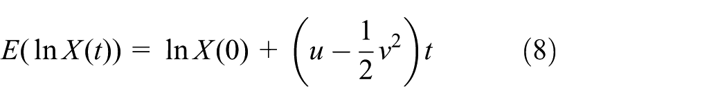
Assume that Y(t) = ln X(t, ω), which leads to

\ln X (t) - \ln X (0) = \int_{0}^{t} \frac{dX}{X} + \frac{1}{2} \int_{0}^{t} \frac{- 1}{X^{2}} v^{2} X^{2} ds

(6)

where s is the time variable

Y (t) - Y (0) = \int_{0}^{t} vd W_{s} + \int_{0}^{t} (u - 0.5 v^{2}) ds

According to equations (7) and (8)

\begin{matrix} \int_{0}^{t} ds = t, \int_{0}^{t} d W_{s} = W_{t} - W_{0}, W_{0} = 0 \\ Y (t) = \ln X (0) + (u - \frac{1}{2} v^{2}) t + vW (t) \end{matrix}

(7)

E (\ln X (t)) = \ln X (0) + (u - \frac{1}{2} v^{2}) t

(8)

We can obtain

\begin{array}{l} \ln E (X (t)) = \ln [E (X (0)) e^{(u - \frac{1}{2} v^{2}) t + v W (t)}] \\ = \ln X (0) + (u - \frac{1}{2} v^{2}) t + \ln e^{0.5 v \sqrt{t}} \end{array}

(9)

The relationship between the expected logarithm and logarithmic expectation can be obtained by

\ln E (X (t)) = \frac{E (\ln X (t)) + D (\ln X (t))}{2}

(10)

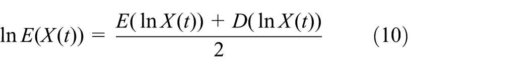
By substituting equation (10) in equations (8) and (9), we can obtain

D (\ln X (t)) = v \sqrt{t}

where ln X(t) is a normal distribution function, and the corresponding mean value and variation coefficient are $\ln X (0) + (u - v^{2} / 2) t$ and $v \sqrt{t}$ , respectively

\ln X (t) ~ N [\ln X (0) + (u - \frac{1}{2} v^{2}) t, v^{2} t]

(11)

Assume that the limit state function is

G (t, ω) = S (t) - δ (t)

(12)

where G(t, ω) > 0 means the structure is safe, and G(t, ω) < 0 indicates failure of the structure. Therefore, the reliability probability is expressed as

R (t) = P (\ln S (t) - \ln δ (t) > 0)

Let $Z = \ln S (t) - \ln δ (t)$ , and ln S(t) and ln δ(t) are independent from each other. Thus, Z also obeys normal distribution. The mean value and variance of Z are expressed as

u_{Z} = u_{\ln S (t)} - u_{\ln δ (t)}

(13)

σ_{Z} = \sqrt{σ_{\ln S (t)} + σ_{\ln δ (t)}}

(14)

Then, the probability density function of Z is

ϕ (Z) = \frac{1}{\sqrt{2 π} σ_{Z}} e^{\frac{- {(Z - u_{Z})}^{2}}{2 σ_{Z}^{2}}}

(15)

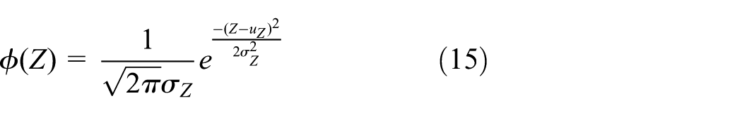
Let $s = (Z - u_{Z}) / σ_{Z}$ . Since reliability index can be expressed as

\begin{array}{l} R (t) = P (Z > 0) = \int_{0}^{\infty} ϕ (Z) d Z = \sqrt{2 π} \int_{Z_{R (t)}}^{\infty} e^{- 0.5 s^{2}} d s \\ = \sqrt{2 π} \int_{- \infty}^{- Z_{R (t)}} e^{- 0.5 s^{2}} d s \end{array}

The reliability index can be obtained by R(t) = Φ(−Z_R_(t)). Substitute equation (15) in equations (13) and (14)

Z_{R (t)} = - \frac{u_{\ln S (t)} - u_{\ln δ (t)}}{\sqrt{σ_{\ln S (t)} + σ_{\ln δ (t)}}}

(16)

where

u_{\ln S (t)} - u_{\ln δ (t)} = \ln S (0) + (u_{S} - 0.5 v_{S}^{2}) t - (\ln δ (0) + (u_{δ} - 0.5 v_{δ}^{2}) t)

and

\begin{array}{l} \ln S (0) - \ln δ (0) = - Z_{R (t)} \sqrt{σ_{\ln S (t)} + σ_{\ln δ (t)}} + ((u_{S} - 0.5 v_{S}^{2}) - (u_{δ} - 0.5 v_{δ}^{2})) t \frac{S (0)}{δ (0)} \\ = \exp {- Z_{R (t)} \sqrt{σ_{\ln S (t)}^{2} + σ_{\ln σ (t)}^{2}} - [(u_{s} - \frac{1}{2} v_{s}^{2}) - (u_{δ} - \frac{1}{2} v_{δ}^{2})] t} \end{array}

(17)

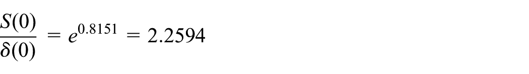
Once the reliability index Z_R_(t) is given, take initial S(0) and δ(0) as constrains to quantify time-varying uncertainties, and the time-varying reliability optimization model can be constructed.

Time-varying reliability MDO

Multidisciplinary simultaneous analysis and design

Generally, a multidisciplinary optimization problem consists of two subsystems. The multidisciplinary simultaneous analysis and design (SAND) method³³ is introduced to construct the optimization framework, which is shown in Figure 2. Since time-varying uncertainties analysis is complicated and time-consuming, it is better to combine it with simple and easy MDO strategy. Compared to the other MDO strategies, SAND expression is simpler and easier to understand. SAND strategy can substitute solver for analyzer, which can reduce the high time-consuming analysis process.

Figure 2.

SAND optimization framework.

In Figure 2, X_s and P_s are the shared design variable vector and shared design parameter vector, respectively. X_i is the design variable vector of discipline i, P_i is the design parameter vector of discipline i, y_ij is the coupled state variable vector which is the output from i and input to discipline j, and $y'_{ij}$ is the corresponding auxiliary variable vector. g(i) and h(i) represent the inequality and equality constraints of discipline i. m₁ and m₂ are the residuals of coupled state variable and auxiliary variable after the multidisciplinary analysis. SAND optimization strategy passes the values of design variable vector, coupled state variable vector, and auxiliary variable vector to each discipline; according to the values of the design variable vector and auxiliary variable vector, each discipline gets the values of output coupled variable vector after multidisciplinary analysis. At the same time, coupled state variable vector, residuals, and constraints of all disciplines are passed to the optimizer. Using this optimization strategy, each discipline can be analyzed independently. The optimization model of SAND is listed as follows

\begin{matrix} min f (X_{s}, P_{s}, X_{i}, P_{i}, Y) \\ s . t . g^{(i)} (X_{s}, P_{s}, X_{i}, P_{i}, {Y'}_{• i}) \leq 0 \\ h^{(i)} (X_{s}, P_{s}, X_{i}, P_{i}, {Y'}_{• i}) = 0 \\ m_{i} = Y_{i •} - {Y'}_{• i} = 0; i = 1, 2 \\ Y = {y_{12}, y_{21}}; Y' = {{Y'}_{12}, y_{21}^{1}} \\ DV = {X_{s}, X_{i}, Y, Y'} \end{matrix}

(18)

Ito-RBTV-MDO model

The time-varying reliability optimization model of MDO is shown as follows

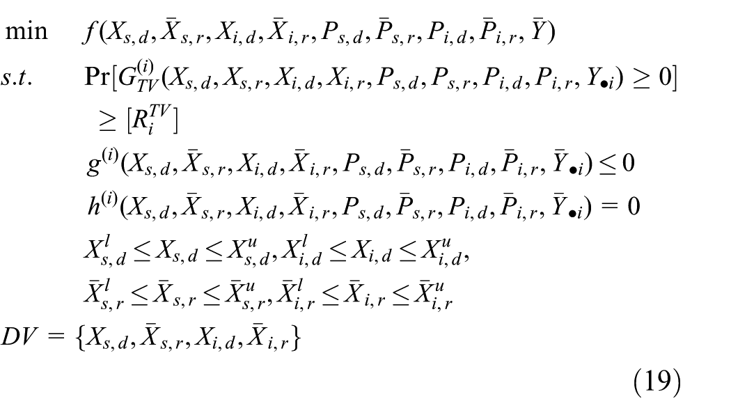
\begin{matrix} min f (X_{s, d}, {\bar{X}}_{s, r}, X_{i, d}, {\bar{X}}_{i, r}, P_{s, d}, {\bar{P}}_{s, r}, P_{i, d}, {\bar{P}}_{i, r}, \bar{Y}) \\ s . t . \Pr [G_{TV}^{(i)} (X_{s, d}, X_{s, r}, X_{i, d}, X_{i, r}, P_{s, d}, P_{s, r}, P_{i, d}, P_{i, r}, Y_{• i}) \geq 0] \\ \geq [R_{i}^{TV}] \\ g^{(i)} (X_{s, d}, {\bar{X}}_{s, r}, X_{i, d}, {\bar{X}}_{i, r}, P_{s, d}, {\bar{P}}_{s, r}, P_{i, d}, {\bar{P}}_{i, r}, {\bar{Y}}_{• i}) \leq 0 \\ h^{(i)} (X_{s, d}, {\bar{X}}_{s, r}, X_{i, d}, {\bar{X}}_{i, r}, P_{s, d}, {\bar{P}}_{s, r}, P_{i, d}, {\bar{P}}_{i, r}, {\bar{Y}}_{• i}) = 0 \\ X_{s, d}^{l} \leq X_{s, d} \leq X_{s, d}^{u}, X_{i, d}^{l} \leq X_{i, d} \leq X_{i, d}^{u}, \\ {\bar{X}}_{s, r}^{l} \leq {\bar{X}}_{s, r} \leq {\bar{X}}_{s, r}^{u}, {\bar{X}}_{i, r}^{l} \leq {\bar{X}}_{i, r} \leq {\bar{X}}_{i, r}^{u} \\ DV = {X_{s, d}, {\bar{X}}_{s, r}, X_{i, d}, {\bar{X}}_{i, r}} \end{matrix}

(19)

where X_s,d and P_s,d are the shared deterministic design variable vector and shared deterministic design parameter vector, respectively. X_i,d and P_i,d are the shared deterministic design variable vector and shared deterministic design parameter vector of discipline i, respectively. X_s,r and P_s,r are the shared random variable vector and shared random parameter vector, respectively. X_i,r and P_i,r are the shared random variable vector and shared random parameter vector of discipline i, respectively. $\bar{X}$ is the mean value of X. $G_{TV}^{(i)} (•)$ is the limit state function by considering time-varying uncertainties. $\Pr [G_{TV}^{(i)} (\cdot) > 0]$ ≥ [R_i] is the time-varying reliability constraint of discipline i, and [ $R_{i}^{TV}$ ] is the reliability requirement of discipline i.

The two subsystems Ito-reliability-based time varying (RBTV)-MDO model is shown in Figure 3.

Figure 3.

Ito-RBTV-MDO optimization framework.

In Figure 3, $g_{\Pr}^{(i)}$ is the time-varying reliability constraint equation of discipline i. The optimization process is given as follows:

Step 1. Deterministic MDO is implemented using the SAND method.

Step 2. Time-varying uncertainties are analyzed and quantified (the data of time-varying uncertainties are obtained by simulate sampling method in this article).

Step 3. Apply Ito equation theory to construct reliability optimization models under time-varying uncertainties.

Step 4. Convert time-varying reliability optimization models to constraints in MDO and implement a new deterministic MDO.

The corresponding flow chart is shown in Figure 4.

Figure 4.

Time-varying reliability optimization flow chart.

Case studies

In this section, both a mathematical example and a case study of an engineering system are introduced to illustrate feasibility and validity of the proposed method.

A mathematical example

This is a very classic MDO problem which includes two disciplines. Each discipline has a coupled state variable; nonlinear coupled relationship exists between two disciplines.³⁴ In order to reflect actual situation more clearly, we have modified this mathematical example. Two time-varying uncertainties p₁ and p₂ are added in optimization model, which to research how system limit state function G(t, ω) are effected.

The optimization model is expressed as follows

\begin{matrix} Min f = (x_{1} - 1.2)^{2} + (x_{2} - 1.5)^{2} + y_{1} + e^{- y_{2}} - p_{1} p_{2} \\ s . t . g_{1} = (\frac{y_{1}}{3.16}) - 1 \geq 0 \\ g_{2} = 1 - (\frac{y_{2}}{24}) \geq 0 \end{matrix}

where

\begin{matrix} y_{1} = x_{1} + x_{2} + x_{3}^{2} - 0.2 y_{2} - p_{1} p_{2} \\ y_{2} = \sqrt{y_{1}} + x_{2} + x_{3} + p_{1} p_{2} \end{matrix}

The corresponding SAND model is shown in Figure 5.

Figure 5.

SAND model of mathematical example.

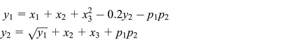
The corresponding limit state function is given by $G (t, ω) = (p_{1} (t, ω) + 0.2) (p_{2} (t, ω) + 0.4) - x_{1} x_{2} x_{3}$ . In this mathematical example, we only consider how the system performance is affected by time-varying uncertainties. How to establish a reasonable and scientific limit state function in the practical engineering problems depends on the requirements of system performance in design stage.

The design parameters p₁ and p₂ are time-varying uncertainties. The corresponding sampling data are obtained by MATLAB simulation during 10 years, which is shown in Figure 6.

Figure 6.

Time-varying data of two design parameters.

Using equations (3) and (4), to calculate the drift rates and fluctuation rates

\begin{matrix} u_{p_{1}} = - 0.000926; v_{p_{1}} = 0.012 \\ u_{p_{2}} = - 0.002; v_{p_{1}} = 0.024 \end{matrix}

State function is expressed as

\begin{matrix} S (t) = (p_{1} (t, ω) + 0.2) (p_{2} (t, ω) + 0.4) \\ δ (t) = x_{1} x_{2} x_{3} \\ R (t) = P (G (t, ω) > 0) = P (\ln S (t) - \ln δ (t) > 0) \end{matrix}

The design requirement of reliability index is 0.998 after 10 years, then

Z_{R (t)} = Z_{R (120)} = - 2.8782

According to equation (17), we have

\frac{S (0)}{δ (0)} = e^{0.8151} = 2.2594

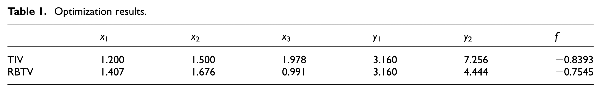
Through updating state equation under time-varying uncertainties and implementing the optimization process mentioned in section “Ito-RBTV-MDO model,” the corresponding optimization results are shown in Table 1, where time invariant (TIV) is the optimization result without considering time-varying uncertainties; RBTV is the reliability optimization result under time-varying uncertainties.

Table 1.

Optimization results.

	x ₁	x ₂	x ₃	y ₁	y ₂	f
TIV	1.200	1.500	1.978	3.160	7.256	−0.8393
RBTV	1.407	1.676	0.991	3.160	4.444	−0.7545

The reliability indexes of state function in each year are shown in Figure 7.

Figure 7.

Comparison of reliability indexes.

From the optimization results of these two methods, we can note that the value of objection function of RBTV method increases by 10.1% than TIVs. However, without considering the time-varying uncertainties, the reliability index of TIV method is 0.8262 after 10 years, which is obviously lower than the reliability index of design requirement 0.998. The reliability index of RBTV method is 0.9999 after 10 years by considering the time-varying uncertainties, which still satisfied the design requirement of reliability.

An engineering example

This is a speed-reducer optimization problem,³⁵ and the structure is shown in Figure 8. The objective function is to minimize the volume of the structure. The main constrains are the bending stress and contact stress of the gear tooth, the torsion deformation, and stress requirements of the shafts.

Figure 8.

Structure diagram of speed reducer.

The corresponding optimization model is as follows

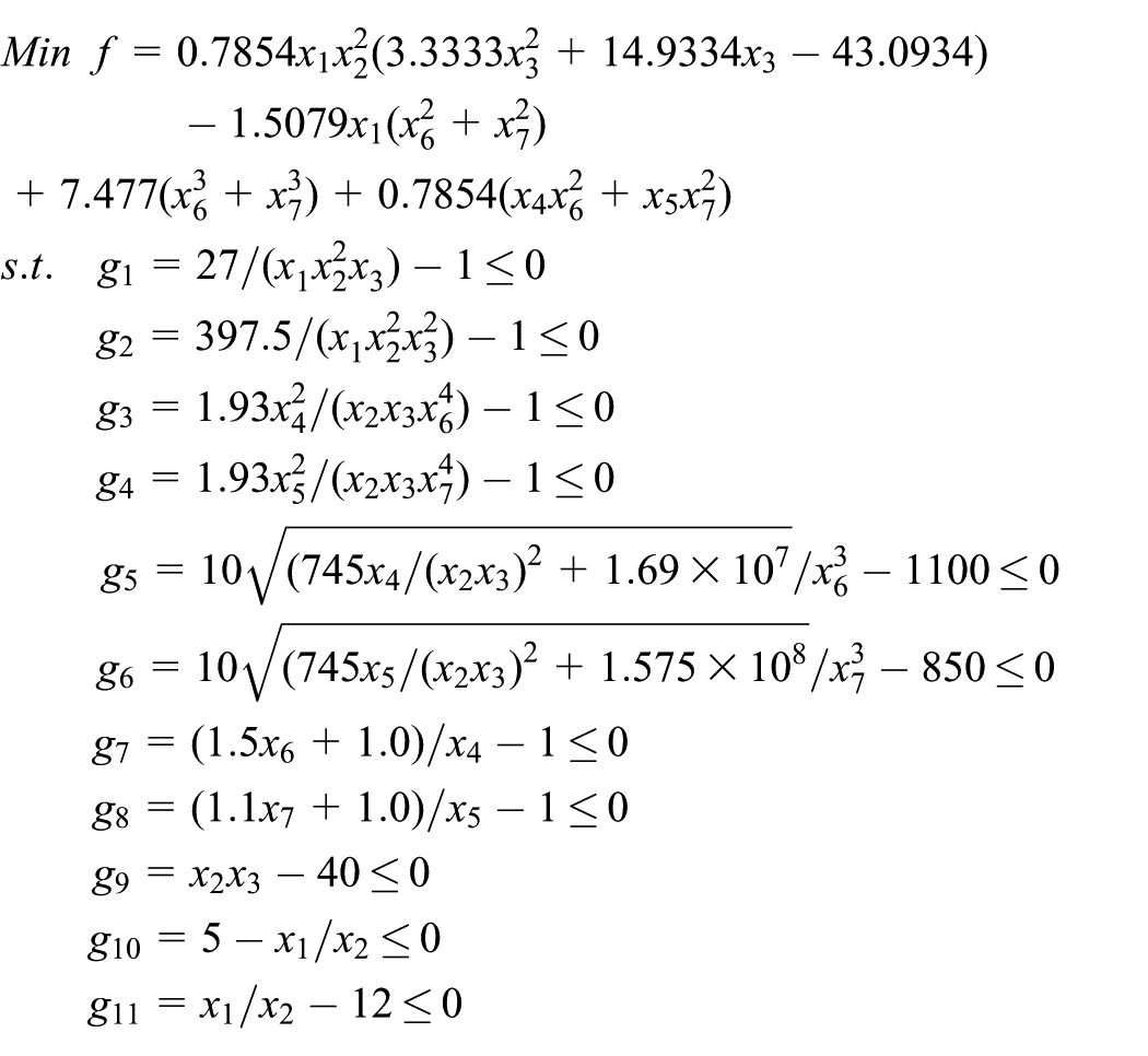
\begin{matrix} Min f = 0.7854 x_{1} x_{2}^{2} (3.3333 x_{3}^{2} + 14.9334 x_{3} - 43.0934) \\ - 1.5079 x_{1} (x_{6}^{2} + x_{7}^{2}) \\ + 7.477 (x_{6}^{3} + x_{7}^{3}) + 0.7854 (x_{4} x_{6}^{2} + x_{5} x_{7}^{2}) \\ s . t . g_{1} = 27 / (x_{1} x_{2}^{2} x_{3}) - 1 \leq 0 \\ g_{2} = 397.5 / (x_{1} x_{2}^{2} x_{3}^{2}) - 1 \leq 0 \\ g_{3} = 1.93 x_{4}^{2} / (x_{2} x_{3} x_{6}^{4}) - 1 \leq 0 \\ g_{4} = 1.93 x_{5}^{2} / (x_{2} x_{3} x_{7}^{4}) - 1 \leq 0 \\ g_{5} = 10 \sqrt{(745 x_{4} / {(x_{2} x_{3})}^{2} + 1.69 \times 10^{7}} / x_{6}^{3} - 1100 \leq 0 \\ g_{6} = 10 \sqrt{(745 x_{5} / {(x_{2} x_{3})}^{2} + 1.575 \times 10^{8}} / x_{7}^{3} - 850 \leq 0 \\ g_{7} = (1.5 x_{6} + 1.0) / x_{4} - 1 \leq 0 \\ g_{8} = (1.1 x_{7} + 1.0) / x_{5} - 1 \leq 0 \\ g_{9} = x_{2} x_{3} - 40 \leq 0 \\ g_{10} = 5 - x_{1} / x_{2} \leq 0 \\ g_{11} = x_{1} / x_{2} - 12 \leq 0 \end{matrix}

where x₁ is the tooth width; x₂ is the gear module; x₃ is the number of teeth of the pinion; x₄ is the distance between the bearings 1; x₅ is the distance between bearings 2; x₆ is the diameter of the shaft 1; x₇ is the diameter of the shaft 2; g₁ and g₂ are the constraints of bending stress and contact stress, respectively; g₃–g₈ are the constraints of the shaft deformation, stress, and so on; and g₉–g₁₁ are the geometric constraints. The bounds of each design variable are shown in Table 2.

Table 2.

Lower and upper bounds of design variables (mm).

Design variables	x ₁	x ₂	x ₃	x ₄	x ₅	x ₆	x ₇
Value range	2.6–3.6	0.7–0.8	17–28	7.3–8.3	7.3–8.3	2.9–3.9	5.0–5.5

The limit state functions of g₅ and g₆ are as follows

\begin{matrix} G_{1} (t, ω) = 1100 x_{6}^{3} - 10 \sqrt{(745 x_{4} / {(x_{2} x_{3})}^{2} + 1.69 \times 10^{7}} \\ G_{2} (t, ω) = 850 x_{7}^{3} - 10 \sqrt{(745 x_{5} / {(x_{2} x_{3})}^{2} + 1.575 \times 10^{8}} \end{matrix}

Assuming that design variables x₆ and x₇ are time-varying uncertainties. The corresponding data of time-varying uncertainties are obtained by simulation methods, which are shown in Figure 9.

Figure 9.

Time-varying data.

Using equations (3) and (4) to calculate the drift rate and fluctuation rate

\begin{matrix} u_{x_{6}} = - 0.0001207; v_{x_{6}} = 0.001092 \\ u_{x_{7}} = - 0.00007335; v_{x_{7}} = 0.0005607 \end{matrix}

Let us consider

\begin{matrix} S_{1} (t) = 1100 x_{6}^{3}, δ_{1} (t) = 10 \sqrt{(745 x_{4} / {(x_{2} x_{3})}^{2} + 1.69 \times 10^{7}} \\ S_{2} (t) = 850 x_{7}^{3}, δ_{2} (t) = 10 \sqrt{(745 x_{5} / {(x_{2} x_{3})}^{2} + 1.575 \times 10^{8}} \\ R_{1} (t) = P (G_{1} (t, ω) > 0) = P (\ln S_{1} (t) - \ln δ_{1} (t) > 0) \\ R_{2} (t) = P (G_{2} (t, ω) > 0) = P (\ln S_{2} (t) - \ln δ_{2} (t) > 0) \end{matrix}

Suppose 1 year later, the requirement of reliability index is 0.98, then

Z_{R_{1} (t)} = Z_{R_{2} (t)} = Z_{R (12)} = - 2.0538

According to equation (17)

\begin{matrix} \frac{S_{1} (0)}{δ_{1} (0)} = e^{0.3932} = 1.4817 \\ \frac{S_{2} (0)}{δ_{2} (0)} = e^{0.2018} = 1.2236 \end{matrix}

The corresponding optimization results are shown in Table 3. TIV is the optimization result without considering time-varying uncertainties; RBTV is the reliability optimization result under time-varying uncertainties.

Table 3.

Optimization results.

	x ₁	x ₂	x ₃	x ₄	x ₅	x ₆	x ₇	g ₅	g ₆	f
TIV	3.5	0.7	17	7.3	7.715	3.35	5.287	1.032E−8	0	2994.2
RBTV	3.5	0.7	18	7.3	7.716	3.35	5.287	−0.5142	−0.2345	3171.7

The reliability indexes of limit state functions in each month are shown in Figure 10.

Figure 10.

Reliability indexes of g₅ and g_6.

Without considering the time-varying uncertainties, the reliability indexes of g₅ and g₆ are 0.4991 and 0.5010, respectively, at initial time. Considering the time-varying uncertainties, the reliability indexes of g₅ and g₆ are 0.9999 and 0.99140, respectively, at initial time. 1 year later, the reliability indexes of g₅ and g₆ are 0.9987 and 0.9813, which still meet the reliability requirements. Although the value of objective function under time-varying uncertainties is 5.23% higher than the results without considering time-varying uncertainties, the reliability performance under time-varying uncertainties has been greatly improved. From this engineering example, it is worth noting that time-varying uncertainties have shown a great influence on the reliability performance of the system. In practical engineering optimization, the impact of time-varying uncertainties should be properly considered.

Conclusion

The time-varying uncertainties of complex mechanical system are investigated using stochastic process and corresponding time-varying reliability optimization model are proposed.

Using the SAND method, the model of MRDO under time-varying uncertainties is established. Then, a mathematical example and an engineering example are introduced to verify the accuracy and effectiveness of the proposed method.

The proposed method is suitable for estimating gradual time-varying uncertainties, such as fatigue strength and material wear, which is not suitable for mutational time-varying uncertainties, such as mutational load and stress. As for mutational time-varying uncertainties, it may be calculated by combining extreme value theory with series reliability analysis method.

Due to the complexity of MDO, diverse manifestations, and correlation of time-varying uncertainties, it is very difficult to quantify the characteristics of time-varying uncertainties in some cases, which will be further investigated.

Footnotes

Academic Editor: Yongming Liu

Declaration of conflicting interests

The author(s) declared no potential conflicts of interest with respect to the research, authorship, and/or publication of this article.

Funding

The author(s) disclosed receipt of the following financial support for the research, authorship, and/or publication of this article: This research was supported by the National Natural Science Foundation of China under the contract no. 51475082.

References

Edward

Luis

Afzal

Multidisciplinary design optimization of an automotive magnetorheological brake design. Comput Struct 2008; 86: 207–216.

Timothy

Joaquim

Multidisciplinary design optimization for complex engineered systems: report from a national science foundation workshop. J Mech Des: T ASME 2011; 133: 1–10.

Mathieu

Nicolas

Philippe

. A survey of multidisciplinary design optimization methods in launch vehicle design. Struct Multidiscip O 2012; 45: 619–642.

Anand

Deshmukh James

. Multidisciplinary dynamic optimization of horizontal axis wind turbine design. Struct Multidiscip O 2016; 53: 15–27.

Chen

Methodology for uncertainty propagation and management in simulation-based systems design. AIAA J 2000; 38: 1471–1478.

Chen

Efficient uncertainty analysis methods for multidisciplinary robust design. AIAA J 2002; 40: 545–552.

Renaud

Batill

. Worst case propagated uncertainty of multidisciplinary systems in robust design optimization. Struct Multidiscip O 2000; 20: 190–213.

Gao

Xie

Fuzzy dynamic reliability models of parallel mechanical systems considering strength degradation path dependence and failure dependence. Math Probl Eng 2015; 2015: 1–9.

Xie

Wang

. Reliability degradation of mechanical components and systems. In: Misra

(ed.) Handbook of performability engineering. London: Springer, 2008, pp.413–429.

10.

Zhu

Huang

Smith

. Bayesian framework for probabilistic low cycle fatigue life prediction and uncertainty modeling of aircraft turbine disk alloys. Probabilist Eng Mech 2013; 34: 114–122.

11.

Zhu

Huang

Ontiveros

. Probabilistic low cycle fatigue life prediction using an energy-based damage parameter and accounting for model uncertainty. Int J Damage Mech 2012; 21: 1128–1153.

12.

Son

YK.

Reliability prediction of engineering systems with competing failure modes due to component degradation. J Mech Sci Technol 2011; 25: 1717–1725.

13.

Zhang

Xiao

Kang

Degradation prediction model based on a neural network with dynamic windows. Sensors 2015; 15: 6996–7015.

14.

Zhu

Huang

Peng

. Probabilistic Physics of Failure-based framework for fatigue life prediction of aircraft gas turbine discs under uncertainty. Reliab Eng Syst Safe 2016; 146: 1–12.

15.

Zhu

Huang

. Probabilistic modeling of damage accumulation for time-dependent fatigue reliability analysis of railway axle steels. Proc IMechE, Part F: J Rail and Rapid Transit 2015; 229: 23–33.

16.

Melchers

RE.

Structural reliability analysis and prediction. Chichester: John Wiley & Sons, 1999.

17.

Veneziano

Grigoriu

Cornell

CA.

Vector-process models for system reliability. J Eng Mech Div: ASCE 1977; 103: 441–460.

18.

Breitung

Rackwitz

Nonlinear combination of load processes. Mech Based Des Struc 1982; 10: 145–166.

19.

Breitung

Asymptotic crossing rates for stationary Gaussian vector processes. Stoch Proc Appl 1988; 29: 195–207.

20.

Breitung

. The extreme value distribution of non-stationary vector processes. In: Proceedings of the 5th international conference on structural safety and reliability (ICOSSAR), San Francisco, CA, 7–11 August 1989, pp.1327–1332. American Society of Civil Engineers.

21.

Breitung

. Asymptotic approximations for the crossing rates of Poisson square waves. In: Proceedings of the conference on extreme value theory and applications, May 1993, pp.82–90. Gaithersburg, MD: NIST Special Publication.

22.

Zhang

YM.

Time-variant reliability assessment and its sensitivity analysis of cutting tool under invariant machining condition based on Gamma process. Math Probl Eng 2012; 2012: 542–551.

23.

Shinozuka

Probability of failure under random loading. J Eng Mech: ASCE 1964; 90: 147–171.

24.

Andrieu-Renaud

Sudret

Lemaire

The PHI2 method: a way to compute time-varying reliability. Reliab Eng Syst Safe 2004; 84: 75–86.

25.

Cazugu

Renaud

Cognard

JY.

Time-varying reliability of nonlinear structures: application to a representative part of a plate floor. Qual Reliab Eng Int 2006; 22: 101–118.

26.

Mourelatos

ZP.

Time-dependent reliability estimation for dynamic problems using a niching genetic algorithm. J Mech Design 2009; 131: 1–13.

27.

Jiang

Han

. Non-probabilistic convex model process: a new method of time-variant uncertainty analysis and its application to structural dynamic reliability problems. Comput Method Appl M 2014; 268: 656–676.

28.

Wehenkel

Lebrevelec

Trotignon

. Probabilistic design of power-system special stability controls. Control Eng Pract 1999; 7: 183–194.

29.

Yasumasa

Fabrizio

Roberto

Probabilistic design of LPV control systems. Automatica 2003; 39: 1323–1337.

30.

Wen

YK.

Reliability-based design under multiple loads. Struct Saf 1993; 13: 3–19.

31.

Ravindra

Walser

Probabilistic design of nuclear structures: a summary of state of the art and research needs. Nucl Eng Des 1978; 50: 115–122.

32.

Yan

Shi

Time-dependent reliability analysis under uncertainty. J Xi’an Jiaotong Univ 2007; 41: 1303–1306.

33.

Allison

JT.

Complex system optimization: a review of analytic target cascading collaborative optimization, and other formulations. PhD Dissertation, University of Michigan, Ann Arbor, MI, 2004.

34.

Chan

. Evaluation of two concurrent design approaches in multidisciplinary design optimization. NRC report, report no. LM-A-077, Canadian Aeronautics and Space Institute, January 2001.

35.

Shayanfar

Abbasnia

Khodam

Development of a GA-based method for reliability-based optimization of structures with discrete and continuous design variables using OpenSees and Tcl. Finite Elem Anal Des 2014; 90: 61–73.

Multidisciplinary reliability design optimization under time-varying uncertainties

Abstract

Keywords

Introduction

Time-varying reliability model

Reliability analysis under time-varying uncertainties

Stochastic differential equation

Time-varying reliability model

Time-varying reliability MDO

Multidisciplinary simultaneous analysis and design

Ito-RBTV-MDO model

Case studies

A mathematical example

An engineering example

Conclusion

Footnotes

Declaration of conflicting interests

Funding

References