Oscillation design of sampling proportional–derivative sliding-mode systems for linear plants with hysteresis

Abstract

This article deals with the self-sustained oscillation appearing in the sliding-mode system. The oscillation provides considerable robust performance and, meanwhile, leads to detrimental effects such as the reduced control precision, mechanical wear, and resonance. A graphical method is introduced to design the sliding-mode controller with proportional–derivative terms. The method indicates how to determine the proportional–derivative coefficients and the desired oscillation frequency and amplitude for the stability of systems. The analysis shows that the zero-order holder plays an important role in the robustness of systems which can be improved by shorter sampling periods. The influences of the hysteresis on the oscillations are also discussed, and a method of tuning the coefficients of proportional–derivative terms is used to compensate the hysteresis. The first simulation shows the design processes of the graphical method in a specific system, and the second simulation confirms the validity of the method of hysteresis compensation. The design process is also demonstrated via the experiment on an inverted pendulum.

Introduction

Sliding-mode (SM) control is insensitive to disturbances and usually simple to implement. Especially, the oscillation with high frequency in SM control is able to provide sufficient gain and improves the performance of disturbance attenuation for a system.^1,2 Hence, the robustness of an SM control system can be enhanced by increasing the oscillation frequency. However, the main drawback of an SM system is mainly related to the oscillation caused by the nonlinear element. ³ It may reduce the control precision, induce resonances, and exceed the maximum switching rate of the controller. Hence, how to design and adjust the oscillation parameters including amplitude A_n and frequency ω_n remains an issues of great importance in SM system design. ⁴

The design of sliding surfaces is closely related to oscillation parameters. The ideal sliding surface is designed by all state variables which can be measured directly without noise.^5,6 Therefore, the oscillation parameters of this SM system can be adjusted straightforwardly. However, in the practical implementation, the high-order state variables are usually unmeasurable or full of noise. In this case, the output feedback sliding surface is another feasible choice, which only needs the output of the plant.^7,8 The complexity of the system can be accordingly reduced by less feedback information. However, it is challenging for the system to adjust the oscillations when the relative degree is ≥2. Consequently, the well-known second-order SM systems often employ this type of sliding surfaces.

However, the parasitic dynamics, such as the zero-order holder (ZOH) and hysteresis, are also crucial components to affect the practical implementation of SM systems. Because of the presence of parasitic dynamics, the SM systems cannot obtain the desired oscillations which provide the required control gain and disturbance attenuation. The influence of parasitic dynamics on the SM system has been thoroughly investigated, ⁹ and the model of fractal dynamics was proposed to analyze the oscillation and nonideal closed-loop performance in the time domain and frequency domain, respectively. The ZOH discretization in SM systems was regarded as an important effect on the periodic orbits. It is modeled as differential equations, and multiple types of periodic orbits have been analyzed. ¹⁰ The effects of the hysteresis on chattering in SM systems are dealt with in the frequency domain via the locus of a perturbed relay system method. The compensating filter is proposed to reject the nonideal effect in a closed-loop SM system. ¹¹

The state–space technique is usually used to describe the process of oscillation. The results are distinct and accurate. ¹² However, the mathematical derivations usually encounter transcendental equations especially for high-order system. The describing function (DF) method is a well-known frequency-domain method for nonlinear system. It approximates the nonlinear element as the function N(A) about the oscillation amplitude. ¹³ The method is effective when the linear plant W(s) has low-pass characteristics. The method has been widely used to estimate the oscillations for nonlinear controller. The stability, dynamic stiffness, and tracking performance of the active disturbance rejection controller were investigated by approximating the nonlinear piecewise function as the DF N(A). ¹⁴ The oscillations in SM system can be regarded as periodic signals. Hence, the DF method is an effective tool to describe the performance of SM system in the frequency domain. The method has been employed to adjust the oscillation parameters and system robustness by tuning the intersection angle of the Nyquist plot of W(s) and the plot of negative reciprocal function −1/N(A). ¹⁵ Currently, a variety of switching functions are analyzed to predict oscillation parameters guided by the DF method. ¹⁶ The oscillations of output feedback SM systems ¹⁷ and second-order SM systems ¹⁸ are also estimated by the DF method in the frequency domain. Using these frequency-domain models, the oscillation parameters can be tuned by the adjustment of coefficients in controller.

This article elaborates the design of oscillation parameters and its adjustment for the sampling output feedback SM controller with proportion–derivative (PD) terms. The main contribution of this work lies in the introduction of the graphical method for the desired oscillation design and the stability analysis in the presence of the ZOH and hysteresis. The method puts forward guidance on the range of coefficient values for the stable oscillation. The effect of the ZOH on the selection of desired oscillation frequency is also demonstrated. In total, three procedures are proposed to design PD coefficients for the predetermined oscillation. The method of hysteresis compensation is also presented for the robust performance by tuning the PD coefficients.

Design of control system

Without loss of generality, a linear plant is considered as follows

$$\{\begin{array}{c}\stackrel{·}{x}\left(t\right)=\mathrm{Ax}\left(t\right)+\mathrm{Bu}\left(t\right)\hfill \\ \multicolumn{1}{c}{y\left(t\right)=\mathrm{Cx}\left(t\right)}\end{array}x\in R^n,y\in R^1$$

(1)

and the SM controller is given by

$$\begin{array}{c}u\left(t\right)=u\prime \left(k{T}_e\right)\hfill \\ u\prime \left(t\right)=u_1\left(t\right)+u_2\left(t\right)\hfill \\ u_1\left(t\right)=M·\mathrm{sign}\left[e\left(t\right)\right]\hfill \\ u_2\left(t\right)=K_{p}e\left(t\right)+K_d\stackrel{·}{e}\left(t\right)\hfill \end{array}$$

(2)

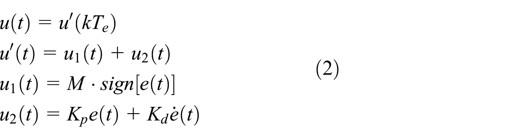
where e(t) = y_r(t) − y(t) is the control error and y_r(t) is the desired system output, M is a positive constant, k is the sampling counter, and T_e is the sampling period. Figure 1 shows the closed-loop system according to equations (1) and (2).

Figure 1.

Diagram of the sampling SM control system.

u ₁(t) comes from the switching function M sign[e(t)], and u₂(t) comes from the linear PD controller. And the SM controller only uses the output of the linear plant. This type of controller is often used in engineering. In general, the PD controller determines the stability of the control system. Besides, the switching function is able to improve the robustness of the system. Therefore, the performance of the system can be tuned by adjusting the coefficients M, T_e, K_p, and K_d. However, there exists interaction between u₁ and u₂. Hence, it is noted that one could not improve performances by tuning any one of these coefficients.

Model of system in the frequency domain

This section illustrates the modeling process in the frequency domain. Suppose that Figure 1 can be divided into linear and nonlinear elements. The linear element is the composition of the linear plant W₁(s) and the ZOH W₂(s). Hence, this element can be represented as follows

$$W\left(s\right)=W_1\left(s\right)·W_2\left(s\right),W_1\left(s\right)=C{(\mathrm{sI}-A)}^{-1}B,W_2\left(s\right)=e^{-s{T}_e}$$

(3)

The nonlinear element N contains the PD term and the switching function. The signals e(t) and u′(t) are the input and output of N, respectively. N can be approximated as a DF by the first harmonic of its output u′(t). First, assume that a periodic signal A sin(ωt) is applied to the input of N. After the corresponding operators, u₁(t) = M sign[A sin(ωt)] and u₂(t) = K_p A sin(ωt) +K_dAω cos(ωt). Then, the nonlinear element N can be represented as equation (4) by the fundamental harmonic Fourier series

$$N(A,\omega )=\frac{1}{\pi A}\underset{0}{\overset{2\pi /\omega }{\int }}u\prime \left(t\right)\sin \left(\omega t\right)d\left(\omega t\right)+\frac{1}{\pi A}\underset{0}{\overset{2\pi /\omega }{\int }}u\prime \left(t\right)\cos \left(\omega t\right)d\left(\omega t\right)=\underset{b_1}{\underbrace{\frac{4M}{\pi A}+K_p}}+j\underset{a_1}{\underbrace{\omega K_d}}$$

(4)

It is noted that the amplitude and frequency values jointly determine the coupled DF N(A, ω) mentioned above. Hence, the N(A, ω) is more complex compared with the uncoupled DF N(A) which only relates to the amplitude A. Consequently, this article suggests a graphical method to design coefficients M, T_e, K_p, and K_d for the stability and the desired oscillation.

Coefficient design and stability analysis

Coefficient design

The closed-loop transfer function of Figure 1 is given by

$$\Phi \left(s\right)=\frac{W\left(s\right)N(A,\omega )}{1+W\left(s\right)N(A,\omega )}$$

(5a)

Hence, the characteristic equation of Figure 1 can be rewritten as follows

$$W\left(j\omega \right)=-\frac{1}{N(A,\omega )}$$

(5b)

where the negative reciprocal function −1/N(A, ω) is obtained by

$$-\frac{1}{N(A,\omega )}=\frac{-(\frac{4M}{\pi A}+K_p)+j\omega K_d}{{(\frac{4M}{\pi A}+K_p)}^2+{\left(\omega K_d\right)}^2}$$

(6)

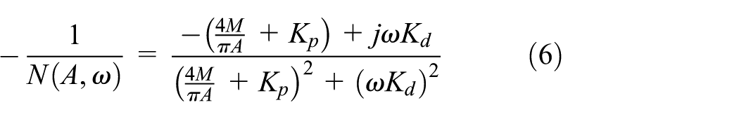
When ω is set as the desired value ω_n, the slope of −1/N(A, ω_n) in the complex plane is not a fixed number with the increase in A. The intersection of −1/N(A, ω_n) and the Nyquist plot W(jω) determines the solution of the oscillation parameters (A_n, ω_n) as shown in Figure 2.

Figure 2.

Example of the Nyquist plots of W(jω) and −1/N(A, ω_n).

In the following, three steps of the graphical method can be used to design K_p, K_d, and M for the desired oscillation (A_n, ω_n):

• Step 1. Set ω and A as the desired frequency ω_n and amplitude A_n, then it is possible to obtain the desired oscillation under the condition that equation (7) holds

$$\{\begin{array}{c}\frac{-(\frac{4M}{\pi A_n}+K_p)}{{(\frac{4M}{\pi A_n}+K_p)}^2+{\left({\omega }_n{K}_d\right)}^2}=\mathrm{Re}\left[W\left(j{\omega }_n\right)\right]\hfill \\ \multicolumn{1}{c}{\frac{{\omega }_n{K}_d}{{(\frac{4M}{\pi A_n}+K_p)}^2+{\left({\omega }_n{K}_d\right)}^2}=\mathrm{Im}\left[W\left(j{\omega }_n\right)\right]}\end{array}$$

(7)

• Step 2. Suppose X = (4M/πA_n) + K_p and Y = ω_nK_d, then one straightforward can obtain X and Y as follows

$$\{\begin{array}{c}X=\frac{-\mathrm{Re}\left[W\left(j{\omega }_n\right)\right]}{{\mathrm{Re}}^2\left[W\left(j{\omega }_n\right)\right]+{\mathrm{Im}}^2\left[W\left(j{\omega }_n\right)\right]}\hfill \\ \multicolumn{1}{c}{Y=\frac{-\mathrm{Im}\left[W\left(j{\omega }_n\right)\right]}{{\mathrm{Re}}^2\left[W\left(j{\omega }_n\right)\right]+{\mathrm{Im}}^2\left[W\left(j{\omega }_n\right)\right]}}\end{array}$$

(8)

Hence, K_p and K_d can be set as

$$\{\begin{array}{c}{K}_d=\frac{1}{{\omega }_n}·\frac{\mathrm{Im}\left[W\left(j{\omega }_n\right)\right]}{{\mathrm{Re}}^2\left[W\left(j{\omega }_n\right)\right]+{\mathrm{Im}}^2\left[W\left(j{\omega }_n\right)\right]}\hfill \\ \multicolumn{1}{c}{K_p=\frac{-\mathrm{Re}\left[W\left(j{\omega }_n\right)\right]}{{\mathrm{Re}}^2\left[W\left(j{\omega }_n\right)\right]+{\mathrm{Im}}^2\left[W\left(j{\omega }_n\right)\right]}-\frac{4M}{\pi A_n}}\end{array}$$

(9)

• Step 3. The amplitude A_n is assumed as a positive real number. Hence, K_p should be set according to the following inequality constraint

$$K_p<\frac{-\mathrm{Re}\left[W\left(j{\omega }_n\right)\right]}{{\mathrm{Re}}^2\left[W\left(j{\omega }_n\right)\right]+{\mathrm{Im}}^2\left[W\left(j{\omega }_n\right)\right]}$$

(10)

Stability analysis

In this case, the setting ranges of K_p, K_d, and ω_n need more discussion. The open-loop transfer function N(A, ω)W(jω) determines the stability of the system. Using the method called small perturbations of amplitudes, the stability can be judged by the geometrical relations between N(A_n + ΔA, ω)W(jω), N(A_n − ΔA, ω)W(jω) and the point (−1, j0).

When W₁(s) is a minimum phase plant, the system must be unstable if N(A_n, ω)W(jω)|_ω = 0 is a negative real number. Hence, for a stable system, K_p and M should satisfy the following inequality

$$\frac{4M}{\pi A_n}+K_p>0$$

(11)

By equations (10) and (11), K_p should be tuned in the range

$$-\frac{4M}{\pi A_n}<K_p<\frac{-\mathrm{Re}\left[W\left(j{\omega }_n\right)\right]}{{\mathrm{Re}}^2\left[W\left(j{\omega }_n\right)\right]+{\mathrm{Im}}^2\left[W\left(j{\omega }_n\right)\right]}$$

(12)

The quadrant where the function −1/N(A, ω_n) is located depends on the sign of the terms (4M/πA) + K_p and K_d as shown in Figure 3. When (4M/πA_n) + K_p > 0 and K_d > 0, −1/N(A, ω_n) is located in the second quadrant; when (4M/πA_n) + K_p > 0 and K_d < 0, −1/N(A, ω_n) is located in the third quadrant. Hence, the desired frequency ω_n can be selected such that Re[W(jω_n)] < 0. As shown in Figure 4, setting the desired frequency as ω_n3 or ω_n4 may cause the instability of the system, and the desired frequency ω_n should be selected in the second and third quadrants. However, the selection of ω_n2 is better than the section of ω_n1, because the oscillation corresponding to ω_n2 is faster, which provides better robustness and accuracy. ²

Figure 3.

The curves of −1/N(A, ω) in the complex plane.

Figure 4.

Example of the frequency selection area for the stable system.

It is worth noting that K_p and K_d can be designed as negatives according to the previous analysis, which is not allowed for the minimum phase plant in linear systems. However, the overall gain is 4M/πA_n + K_p, and the stability of the SM system is determined by the small perturbations of amplitude method. Nonetheless, the method cannot distinguish the global stability and local stability. When the output y is far away from the desired oscillation due to the initial condition x₀ or external disturbance, the switching function cannot provide sufficient gain. In other words, equation (11) may not hold before the system convergences to the oscillation (A_n, ω_n). It means that there exists an attraction basin. If the system leaves the attraction basin, its stability does not hold. It is convenient for the control system to enlarge the size of the attraction basin or design the globally stable system by increasing the coefficient K_p.

The method to describe the attraction basin remains to be discussed. The attraction basin in a fuzzy system is illustrated in simulations in Aracil and Gordillo. ¹⁹ It is also estimated in an SM system with multiple limit cycles, ²⁰ but the accuracy is very poor. In this article, the attraction basin is shown in section “Controller design and verification.”

The influence of ZOH

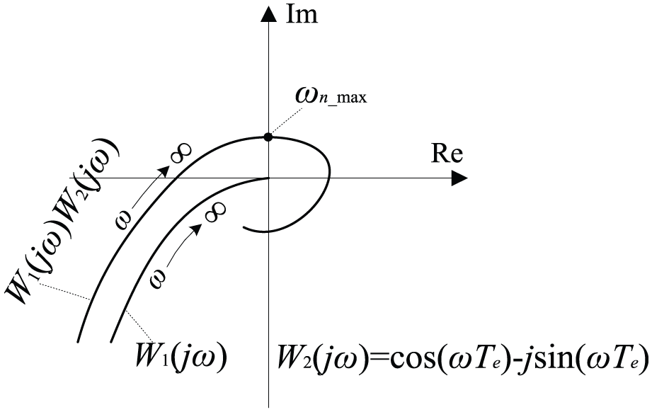
In engineering application, the ZOH is widely used in digital control system. Therefore, the influence of ZOH on the SM controller is discussed in this section. The ZOH leads to a significant change in the Nyquist plot W₁(jω) in the high-frequency band as shown in Figure 5, where the transfer function of ZOH can be represented as W₂(jω) = cos(ωT_e) − j sin(ωT_e). Under the effect of ZOH, the Nyquist plot of W₁(jω)W₂(jω) goes around the origin with the increase in ω. The frequency ω_{n_max} (see Figure 5) is the threshold and ω_{n_max} = π/(2T_e). It is not recommended to set the desired frequency greater than ω_{n_max} for the stability of systems. Hence, decreasing the sampling period T_e could increase the maximum possible oscillation frequency, which is able to improve the robustness of the system.

Figure 5.

The change in W₁(jω) in high-frequency band caused by ZOH.

The influence of hysteresis

The nonlinearity hysteresis widely exists in engineering, such as the gear drive and electromagnetic relays. This section discusses the variation of SM oscillations when the ideal switching function is substituted by the rectangular hysteresis as shown in Figure 6. The DF of the SM controller and its negative reciprocal are given by the following form

$$N(A,\omega )=\frac{4M}{\pi A}\sqrt{1-{\left(\frac{a}{A}\right)}^2}+K_p+j[-\frac{4\mathrm{Ma}}{\pi A^2}+\omega K_d]$$

(13a)

$$-\frac{1}{N\left(A,\omega \right)}=-\frac{\frac{4M}{\pi A}\sqrt{1-{\left(\frac{a}{A}\right)}^2}+K_p-j\left[-\frac{4Ma}{\pi A^2}+\omega K_d\right]}{{\left(\frac{4M}{\pi A}\sqrt{1-{\left(\frac{a}{A}\right)}^2}+K_p\right)}^2+{\left(-\frac{4Ma}{\pi A^2}+\omega K_d\right)}^2}$$

(13b)

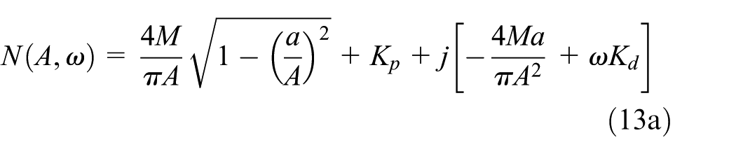
where a is the gap width.

Figure 6.

Nonlinearity of the rectangular hysteresis.

In order to find a more intuitive solution, the graphical depiction is used to analyze the influence of the gap width a on the function −1/N(A, ω_n). −1/N(A, ω_n) without hysteresis as shown in equation (6) is a circular arc with the center O  = (0, 1/2ω_nK_d) and radius r = 1/2ω_nK_d (for proof, see Appendix 1).−1/N(A, ω_n) with gap width a as shown in equation (13b) is also a circular arc with the center O _a and radius r_a (for proof, see Appendix 1), where

$$\begin{array}{l}{\mathrm{O}}_a=\left({\mathrm{O}}_a^X,{\mathrm{O}}_a^Y\right)=\left(\frac{-K_p}{K_p^2+{\left({\omega }_n{K}_d-2M/\pi a\right)}^2-{\left(2M/\pi a\right)}^2},\frac{{\omega }_n{K}_d-2M/\pi a}{K_p^2+{\left({\omega }_n{K}_d-2M/\pi a\right)}^2-{\left(2M/\pi a\right)}^2}\right)\\ r_a=\frac{2M/\pi a}{{\left(2M/\pi a\right)}^2-K_p^2-{\left({\omega }_n{K}_d-2M/\pi a\right)}^2}\end{array}$$

a is a very small number (the gap width in hysteresis is usually very small in the electronic system and machinery); hence, we reasonably assume that 2M/πa > ω_nK_d and 2M/πa>>K_p. Therefore, O _a moves toward the bottom and r_a increases with the increase in a. Figure 7 shows a Nyquist plot of W(jω) and five curves of −1/N(A, ω) with the increase in a. The dashed lines are the contour of amplitudes A. With the increase in the gap width a, the intersections of W(jω) and −1/N(A, ω) move toward the upper left. It means that the gap width a leads to a slower and bigger oscillation which may deteriorate the performance of the controller.

Figure 7.

A cluster curves of −1/N(A, ω) with the variation of the parameter a.

The next topic is how to compensate the hysteresis by tuning K_p and K_d. Because of the insignificance of K_p in O _a and r_a, the variation of K_p almost cannot change the trajectory of −1/N(A, ω). However, K_d is more important than K_p. The curve −1/N(A, ω) moves toward the bottom with the increase in K_d as shown in Figure 8. As a result, the intersection of W(jω) and −1/N(A, ω) moves toward the bottom right with the increase in K_d when a is invariant. It means that the corresponding frequency ω of the intersection could return to the desired ω_n1 as the red line in Figure 7.

Figure 8.

Variation of the curve −1/N(A, ω) with K_d.

Similar to equations (8) and (9), we obtain the compensation coefficients

$$\{\begin{array}{c}{K}_{\mathrm{dc}}=\frac{1}{{\omega }_n}·[\frac{\mathrm{Im}\left[W\left(j{\omega }_n\right)\right]}{{\mathrm{Re}}^2\left[W\left(j{\omega }_n\right)\right]+{\mathrm{Im}}^2\left[W\left(j{\omega }_n\right)\right]}+\frac{4\mathrm{Ma}}{\pi A_n^2}]\hfill \\ \multicolumn{1}{c}{K_{\mathrm{pc}}=\frac{-\mathrm{Re}\left[W\left(j{\omega }_n\right)\right]}{{\mathrm{Re}}^2\left[W\left(j{\omega }_n\right)\right]+{\mathrm{Im}}^2\left[W\left(j{\omega }_n\right)\right]}-\frac{4M}{\pi A_n}\sqrt{1-{\left(\frac{a}{A_n}\right)}^2}}\end{array}$$

(13c)

To compensate the hysteresis, K_dc and K_pc should be enlarged. However, too large K_d may yield negative effects such as the slow response speed.

Numerical simulations

Consider the linear plant given by the state–space model with the matrices

$$A=\left[\begin{array}{ccc}0\hfill & 1\hfill & 0\hfill \\ \multicolumn{1}{c}{0}& 0\hfill & 1\hfill \\ \multicolumn{1}{c}{0}& -2\hfill & -3\hfill \end{array}\right],B=\left[\begin{array}{c}0\hfill \\ \multicolumn{1}{c}{0}\\ \multicolumn{1}{c}{1}\end{array}\right],C={\left[\begin{array}{c}1\hfill \\ \multicolumn{1}{c}{0}\\ \multicolumn{1}{c}{0}\end{array}\right]}^T$$

(14)

The sampling period T_e is set as 10 ms. The model of the linear element (see Figure 1) gives the following transfer function

$$\begin{array}{c}\multicolumn{1}{c}{W\left(s\right)=W_1\left(s\right)W_2\left(s\right)=e^{-\mathrm{sTe}}\frac{1}{s(s+1)(s+2)}}\\ \multicolumn{1}{c}{{W\left(s\right)|}_{s=j\omega }=\frac{\cos \left(\omega T_e\right)-j\sin \left(\omega T_e\right)}{-3{\omega }^2+j(2\omega -{\omega }^3)}}\end{array}$$

(15)

Controller design and verification

The objective of this section is to find the coefficients of the controller such that the oscillation of y satisfies the desired frequency and amplitude. Set the desired oscillation as ω_n1 = 9 rad/s and A_n1 = 0.0075. According to the graphical method, the process of coefficient designing is as follows. First, calculating ω_{n_max} by iterative computations, we obtain that ω_{n_max} = 17.3 rad/s. Based on the analysis in section “The influence of ZOH,” the selection of the desired frequency (ω_n1 = 9 rad/s) does not cause the instability. Next, by equations (7)–(9), we obtain K_d, K_p, and M as follows

$$\begin{array}{c}{K}_d=\frac{1}{{\omega }_{n1}}·\frac{\mathrm{Im}\left[W\left(j{\omega }_{n1}\right)\right]}{{\mathrm{Re}}^2\left[W\left(j{\omega }_{n1}\right)\right]+{\mathrm{Im}}^2\left[W\left(j{\omega }_{n1}\right)\right]}\hfill \\ \multicolumn{1}{c}{=\frac{1.3\times {10}^{-3}}{9\times [{(3.2\times {10}^{-4})}^2+{(1.3\times {10}^{-3})}^2]}=81.1}\\ K_p=\frac{-\mathrm{Re}\left[W\left(j{\omega }_{n1}\right)\right]}{{\mathrm{Re}}^2\left[W\left(j{\omega }_{n1}\right)\right]+{\mathrm{Im}}^2\left[W\left(j{\omega }_{n1}\right)\right]}-\frac{4M}{\pi A_{n1}}\hfill \\ \multicolumn{1}{c}{=\frac{3.2\times {10}^{-4}}{{(3.2\times {10}^{-4})}^2+{(1.3\times {10}^{-3})}^2}-\frac{4M}{\pi A_{n1}}}\end{array}$$

Assuming M = 1, then K_p = 8.4. Finally, by equation (12), we find K_p = 8.4 is an appropriate coefficient. To compare the results of the design, we select a group of values as the desired oscillation parameters as shown in Table 1, and the design results of K_p and K_d are also tabulated in it.

Table 1.

The designed coefficients and the oscillation parameters in simulations.

Designed oscillation		Designed coefficients				Simulated oscillation
Amplitude	Frequency (rad/s)	Te (ms)	M	Kp	Kd	Amplitude	Frequency
An1 = 7.5 × 10−3	ωn1 = 9.0	10	1	8.4	81.1	$A_{n1}^s=6.7\times {10}^{-3}$	${\omega }_{n1}^s=9.1$
An2 = 5.5×10−3	ωn2 = 10.0	10	1	−30.8	100.5	$A_{n2}^s=4.8\times {10}^{-3}$	${\omega }_{n2}^s=10.1$
An3 = 5.5 × 10−3	ωn3 = 12.0	10	1	−6.6	145.3	$A_{n3}^s=4.2\times {10}^{-3}$	${\omega }_{n3}^s=12.1$

In the following, the numerical simulation I is conducted to verify the accuracy of the graphical method. In the simulation, the sampling period T_e is divided into 10 slot times for the higher precision of the derivative de(t)/dt = [e(k) − e(k − 1)]/(0.1 × T_e). The state–space in equation (14) is discretized by G = I + A × T_e/10 and H = B × T_e/10. The controller updates its output u(t) once in every T_e. The coefficients M, T_e, K_p, and K_d in the program are assigned as the designed values in Table 1. The time series, phase portraits, and frequency spectrums of y are plotted in Figure 9(a)–(c), in which the oscillation amplitudes and frequencies can be measured directly. The desired and simulated oscillation parameters are compared in Table 1.

Figure 9.

(a) Time series of designed oscillations, (b) the phase portraits of the three oscillations, (c) spectrum analysis of the steady state of the three oscillations, and (d) the attraction basin of oscillation 2.

The errors between the designed and simulated values may come from the nature of approximation in the frequency-domain method. The accuracy of oscillation parameters A and ω depends on the intensity of residual high-order harmonics which are generated by the switching signal u₁(t) and are suppressed by the low-pass performance of W(s). The errors should be considered as uncertain factors in the design process.

The next issue is to discuss the local stability and attraction basin. Consider the influence of the two state variables x₁ and x₂ on the stability of the system when K_p = −30.8 and K_d = 100.5. Equally spaced initial points are selected in the region R:{−0.1 ≤ x₁ ≤ 0.1, −1 ≤ x₂ ≤ 1, x₃ = 0}, and the steady-state processes corresponding to each point are simulated. We classified the processes as local stability and instability, such as the two trajectories started from points A and B. Then, the region R can be divided into two parts as shown in Figure 9(d). The domain in the red curve is the attraction basin of oscillation 2.

Hysteresis compensation

This section presents the effect of hysteresis on the oscillation and the evaluation of compensation results. Consider a system with the linear plant given by equations (14) and (15) and the controller coefficients K_p = −6.3 and K_d = 41.4. The desired oscillation parameters are A_n1 = 1.1 × 10⁻² and ω_n1 = 6.5 rad/s. In order to agree with our intuition, the Nyquist plots of W(jω) and −1/N₁(A, ω_n1) are shown in Figure 10, and the intersection 1 denotes the desired oscillation (A_n1, ω_n1).

Figure 10.

The graphical illustration of hysteresis compensation.

When the gap width a is set as 3 × 10⁻³, its oscillation becomes (A_n2, ω_n2) = (1.2 × 10⁻², 6.15 rad/s). The curve of function −1/N₂(A, ω_n2) as shown in Figure 10 illustrates that the hysteresis yields a slower and larger oscillation. To compensate the hysteresis, we redesigned K_pc and K_dc according to equation (13c) and obtained K_pc = −1.9 and K_dc = 46.3.

Simulation II is carried out to evaluate the compensation performance. The results are listed in Table 2. We find the enlarged K_d could accelerate the oscillation frequency, and the oscillation amplitude can be adjusted by K_p, which complies with the analysis of section “The influence of hysteresis.”

Table 2.

The evaluation of performance of the hysteresis compensation.

	Theoretical estimation		Hysteresis	Coefficients		Simulation
	Amplitude	Frequency (rad/s)	a	Kp	Kd	Amplitude	Frequency
Ideal system	An 1 = 1.1 × 10−2	ωn 1 = 6.5	0	−6.3	41.4	$A_{n1}^s=9.5\times {10}^{-3}$	${\omega }_{n1}^s=6.54$
Before the compensation	An 2 = 1.2 × 10−2	ωn 2 = 6.15	3 × 10−3	−6.3	41.4	$A_{n2}^s=1.04\times {10}^{-2}$	${\omega }_{n2}^s=6.09$
After the compensation	An 1 = 1.1 × 10−2	ωn 1 = 6.5	3 × 10−3	−1.9	46.3	$A_{n3}^s=9.6\times {10}^{-3}$	${\omega }_{n3}^s=6.4$
	Te = 10 ms; M = 1

Experimental studies

An inverted pendulum device, as shown in Figure 11(a), is employed to test the SM control algorithm and the graphical method. The experimental device contains an AC servo motor with its own speed-loop control. Using the belt transmission, the motor can drive the car on the straight line. The suspended pendulum installed at the car can rotate around the pivot point. The pendulum angle can be measured by the rotary encoder. The coordinate is described in Figure 11(b). The position of the car is denoted by x and the angle of the pendulum is denoted by θ. The device can be managed by Visual C++, including the angle data collection, motor control, and data storage. The algorithm and coefficients can be set by the C++ program. The force F comes from the acceleration of the AC motor which can be set by its speed-loop control. The sampling interval T_e is set as 20 ms for this device.

Figure 11.

(a) Experimental inverted pendulum system and (b) coordinate define.

The motion of the inverted pendulum is described as follows

$$\{\begin{array}{c}(M+m)\stackrel{··}{x}+\mathrm{ml}\stackrel{··}{\theta }=\tau \hfill \\ \multicolumn{1}{c}{\left(\frac{4}{3}\right)m{l}^2\stackrel{··}{\theta }+\mathrm{ml}\stackrel{··}{x}=\mathrm{mgl}\theta }\end{array}$$

(16)

where m = 0.03 kg is the mass of the pendulum, M = 0.7 kg is the mass of the car, l = 0.2 m is the length of the pendulum center from the pivot, g = 9.8 m/s² is the acceleration of gravity, and τ (N) is the control force. Equation (16) can be rewritten as the state–space model as follows

$$\underset{\stackrel{·}{\xi }}{\underbrace{\left[\begin{array}{c}\stackrel{·}{\theta }\hfill \\ \multicolumn{1}{c}{\stackrel{··}{\theta }}\\ \multicolumn{1}{c}{\stackrel{·}{x}}\\ \multicolumn{1}{c}{\stackrel{··}{x}}\end{array}\right]}}=\underset{A}{\underbrace{\left[\begin{array}{cccc}0\hfill & 1\hfill & 0\hfill & 0\hfill \\ \multicolumn{1}{c}{a_1}& 0\hfill & 0\hfill & 0\hfill \\ \multicolumn{1}{c}{0}& 0\hfill & 0\hfill & 1\hfill \\ \multicolumn{1}{c}{a_2}& 0\hfill & 0\hfill & 0\hfill \end{array}\right]}}\underset{\xi }{\underbrace{\left[\begin{array}{c}\theta \hfill \\ \multicolumn{1}{c}{\stackrel{·}{\theta }}\\ \multicolumn{1}{c}{x}\\ \multicolumn{1}{c}{\stackrel{·}{x}}\end{array}\right]}}+\underset{B}{\underbrace{\left[\begin{array}{c}0\hfill \\ \multicolumn{1}{c}{b_1}\\ \multicolumn{1}{c}{0}\\ \multicolumn{1}{c}{b_2}\end{array}\right]}}\underset{u}{\underbrace{\begin{array}{c}\hfill \\ \multicolumn{1}{c}{\tau }\\ \multicolumn{1}{c}{}\end{array}}}$$

(17)

where

$$\begin{array}{c}{a}_1=\frac{(M+m)g}{[(4/3)M+(1/3)m]l}=37.92\hfill \\ a_2=\frac{-\mathrm{mg}}{(4/3)M+(1/3)m}=-0.31\hfill \\ b_1=-\frac{1}{[(4/3)M+(1/3)m]l}=-5.30\hfill \\ b_2=\frac{4}{4M+m}=1.41\hfill \end{array}$$

The output y is defined as y = [1, 0, 0.1, 0]ξ; hence, the transfer function from u to y is written as

$$W_1\left(s\right)=-\frac{5.159(s^2+1.0043)}{s^2(s^2-37.92)}=-{\tilde{W}}_1\left(s\right)$$

(18)

For convenience, ${\tilde{W}}_1(s)$ is regarded as the linear plant. Set two desired oscillations (A_n1, ω_n1) = (1.5 × 10⁻², 15 rad/s) and (A_n2, ω_n2) = (1.5 × 10⁻², 25 rad/s). In accordance with step 1 to step 3 in section “Coefficient design,” we obtain the coefficients: ${\tilde{K}}_{p1}=14.76$ , ${\tilde{K}}_{d1}=1.01$ , and ${\tilde{M}}_1=1$ and ${\tilde{K}}_{p2}=49.29$ , ${\tilde{K}}_{d2}=2.47$ , and ${\tilde{M}}_2=1$ . The Nyquist plots of ${\tilde{W}}_1(s)W_2(s)$ and $-1/N(A,{\omega }_n)$ as shown in Figure 12, graphically illustrate the design.

Figure 12.

The graphical illustration of coefficient design for the inverted pendulum.

To eliminate the minus in equation (18), we have to adjust the coefficients as $K_{p1}=-{\tilde{K}}_{p1}=-14.76$ , $K_{d1}=-{\tilde{K}}_{d1}=-1.01$ , and $M_1=-{\tilde{M}}_1=-1$ and $K_{p2}=-{\tilde{K}}_{p2}=-49.29$ , $K_{d2}=-{\tilde{K}}_{d2}=-2.47$ , and $M_2=-{\tilde{M}}_2=-1$ .

Figure 13(a) displays the experimental oscillations of y in time series. Compared with oscillation 1, oscillation 2 is smaller and faster. It also shows that the disturbance attenuation of oscillation 2 is better because of the higher robustness which is the results of the increment coefficients K_p and K_d. Figure 13(b) shows the spectrum analysis of the periodic motions. Because of the measurement noise and unmodeled dynamics such as friction, the spectrum components of oscillations 1 and 2 distribute at a series of frequencies. However, the main components are located in the ranges of 18.96–21.66 and 23.96–29.46 rad/s, which are close to the designed frequencies as shown in Figure 12.

Figure 13.

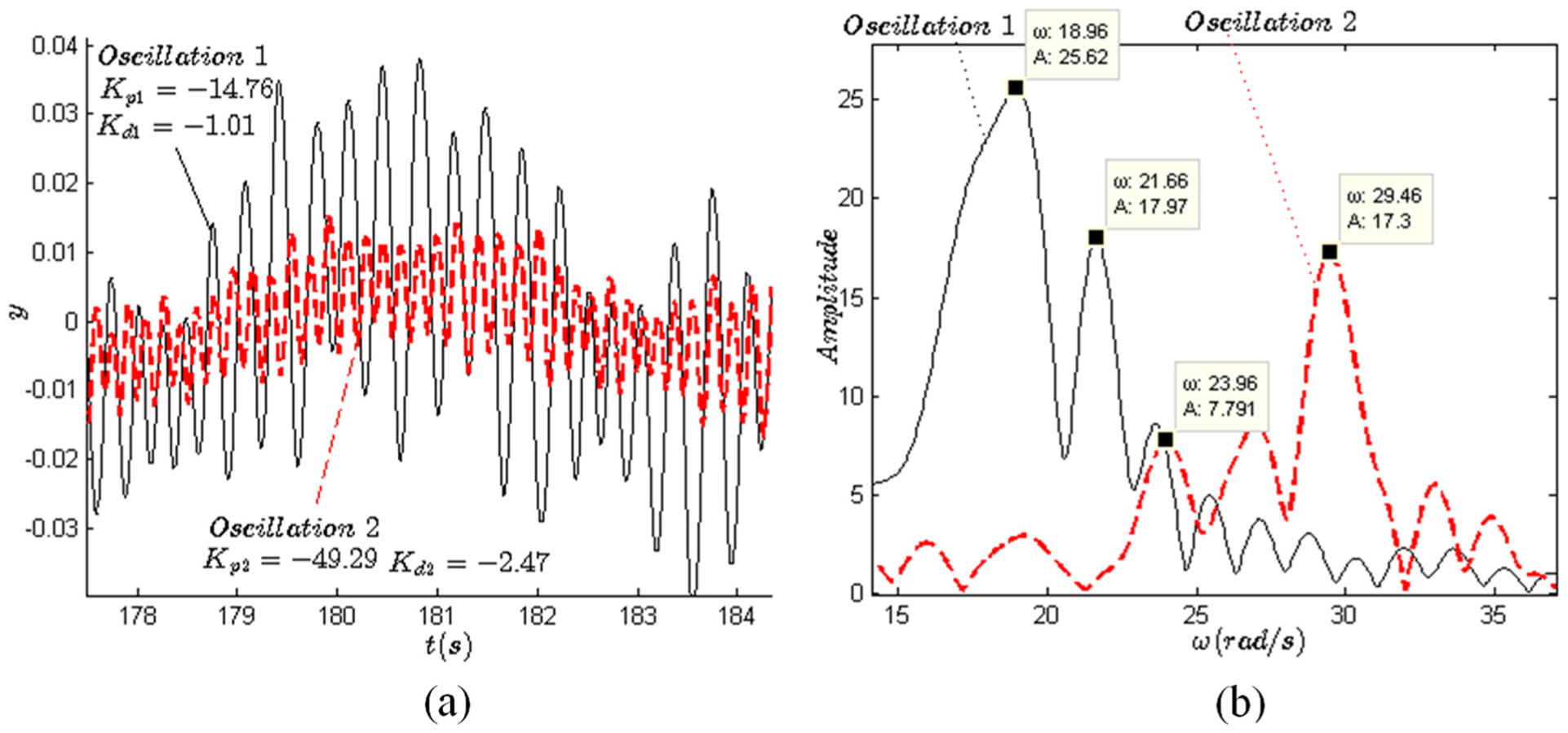
(a) The experimental results of the output y in time series and (b) spectrum analysis of the periodic motions of y.

The experiment shows the importance of the switching function and coefficients K_p and K_d when the feedback information is only x and θ. The switching function is used to guarantee the stability. K_d determines the radius and center of the trajectory −1/N(A, ω) which is closely related to the oscillation frequency. The oscillation amplitude can be flexibly adjusted by K_p.

Conclusion

This article has proposed a frequency-domain technique to analyze and design the characteristic of oscillations in the SM system affected by parasitic dynamics. It also introduces a new control design method in the traditional chattering suppression analysis. It has been shown that the coefficients K_p and K_d in the PD term have remarkable effect on the oscillation frequency and the switching function plays an important role in the stability of the system. The trajectories of −1/N(A, ω) have been accurately described as circular arcs, and the relations of the radius, center, and proportion–derivative coefficients are obtained. The principle of the hysteresis compensation has been demonstrated under the guidance of these relations. Such analysis will give designers insights into how to develop the robustness and stability in terms of various application requirements.

Future work will focus on the estimation of the attraction basin for the locally stable system. This estimation is difficult especially for the high-order system.