Railway rolling bearing fault diagnosis based on multi-scale intrinsic mode function permutation entropy and extreme learning machine classifier

Abstract

The application of the multi-scale intrinsic mode function permutation entropy and extreme learning machine classifiers in railway rolling bearing fault diagnosis is here proposed in this article. The original signal is first denoised using wavelet de-noising as a pre-filter, which improves the subsequent decomposition into a number of intrinsic mode functions using ensemble empirical mode decompose. Second, the multi-scale intrinsic mode function permutation entropy is extracted as feature parameters. Finally, the extracted features are entered into extreme learning machine for an automated fault diagnosis procedure. Case studies have been carried out to evaluate the validity of the approach. The results demonstrate its effectiveness for diagnosis of faults in railway rolling bearings.

Introduction

Rolling bearing is one of the most common mechanical components used in railways. Railway rolling bearings generally perform in harsh environments and can fail easily, which may cause serious damage to the railway. Monitoring the condition of railway rolling bearings is highly significant. ¹ When the railway rolling bearing operates with faults, its dynamic behavior always appears complex and non-stationary, and the signals present corresponding characteristics, which makes the extraction of fault information from the non-stationary and non-linear vibration signals critical issue in the diagnosis of bearing faults. ²

Traditional fault diagnosis algorithms including time-domain and frequency-domain analysis are based on the assumption that the evaluated signals remain stationary and linear throughout the process. This may lead to false results when it is applied to actual bearing fault vibration signals, which may be non-stationary and non-linear. Several time–frequency analyzing methods have been proposed in fault diagnosis of rolling bearings to deal with these non-stationary, non-linear signals. ³ Common time–frequency analysis techniques include Wigner-Ville distribution (WVD), short-time Fourier transform (STFT), and wavelet transform (WT), but each one of these methods has its limitations. For example, WVD can involve crossing-term interference when dealing with the non-stationary signals. The window of analysis of STFT must be optimized further. WT has been commonly applied in health monitoring but different mother wavelets should be predefined for each different component. These drawbacks render these classical methods less than fully adaptive in nature. Empirical mode decompose (EMD) is a self-adaptive time–frequency analysis method. ⁴ Because EMD is capable of dealing with non-linear signals, considerable attention has been drawn to this method in the field of condition monitoring of bearing. However, EMD also has a drawback called modal mixing. It distorts the decomposed intrinsic mode function (IMF). ⁵ In order to solve this problem in the EMD denoising process, Wu and Huang ⁶ proposed ensemble empirical mode decompose (EEMD), which renders it more thorough. EEMD is a time–frequency decomposition technique, which is widely used in fault diagnosis. It presents better performance than the traditional time–frequency analysis in the processing of non-stationary, non-linear signals.

There is considerable consensus that the concept of entropy can be treated as an indicator of the complexity of nonlinear signals. ⁷ Permutation entropy (PE), a parameter of average entropy, can describe the complexity of a time series signal. It is robust under non-linear distortion of the signal with computational efficiency. Multi-scale permutation entropy (MPE), which is based on PE, can describe the complexity of time series within different scales. ⁸

EMD performs well when it used to process nonlinear, non-stationary signals, but it can cause mode mixing during such processes. PE is a measure of complexity. It can be used to detect dynamic mutations of nonlinear signals, but it can only detect the random and dynamic mutation within signal scale. Extreme learning machine (ELM) has the advantages of fast learning speed and good generalization performance. Based on the analysis of both advantages and disadvantages of these methods above, this article presents a method of railway rolling bearing fault diagnosis based on multi-scale IMF PE and ELM classifier. This new method uses EEMD to solve the problem of model mixing to which EMD is subject, and multi-scale PE algorisms are used to solve the issue of single scale problem, and ELM is used to classify the faults. Experiments have confirmed that this method can accurately diagnose the fault of the train bearing. This method provides a theoretical basis for mechanical fault diagnosis and has important practical engineering application value.

The remainder of this article is structured as follows: EMD and EEMD are discussed in section “The EEMD method.” Multi-scale PE is described in section “Multi-scale PE.” In section “ELM method,” ELM is briefly described. In section “Experimental results,” the method is validated experimentally. Finally, conclusions are drawn in section “Conclusion.”

The EEMD method

The EEMD method utilizes the uniform distribution of Gaussian white noise in frequency range and its better performance has been demonstrated with a larger scale separation ability than EMD. ⁹ The EEMD algorithm procedure is given in Figure 1.

Figure 1.

Flowchart of EEMD.

Let

$$x(t)=x_1\left(t\right)+x_2\left(t\right)$$

(1)

$$x_1\left(t\right)=10\sin \left(2\pi 10t\right)$$

(2)

Here, $x_2(t)$ is a discontinuous high frequency sine signal with amplitude of 2 and frequency of 200 Hz. Figure 2 shows the waveforms of $x(t)$ .

Figure 2.

Waveforms of $x(t)$ .

Figures 3 and 4 show the waveforms of each component of EMD and EEMD after $x(t)$ was decomposed. As shown in Figure 3, discontinuous components of signal should only appear in IMF₁ and does not contain low-frequency components, but the actual decomposition results show that IMF₁ contains both discontinuous high-frequency components and partial low-frequency components. Some discontinuous high-frequency components were distributed to IMF₂, which causes notable model mixing; this phenomenon has a serious impact on subsequent signal decomposition. The low-frequency components were mainly distributed to IMF₃ and IMF₄ which causes distortion at both ends of the signal. The decomposed IMF components show that such processes cannot be used to characterize real physical processes. As shown in Figure 4, IMF₁ contained only discontinuous components, and the low-frequency components were distributed to IMF₃. These results showed that EEMD can solve the model mixing problems in EMD decomposition.

Figure 3.

Waveforms of $x(t)$ after EMD decomposition: (a)IMF₁, (b) IMF₂, (c) IMF₃, and (d) IMF₄.

Figure 4.

Waveforms of $x(t)$ after EEMD decomposition: (a)IMF₁, (b) IMF₂, (c) IMF₃, and (d) IMF₄.

Multi-scale PE

MPE proposed by Aziz and Arif ¹⁰ has been employed for the estimation of complexity parameters. The MPE calculates PE over multiple scales to prevent contradictory results using single-scale entropy. This property of MPE makes it more useful for the analysis of non-stationary signals.

First, the original time series data $t=\{t_1,t_2,\dots ,t_N\}$ are converted to multiple successive coarse-grained time series. This objective can be realized by taking the average of the data inside non-overlapping times slice of increasing length t. Coarse-grained time series shown in Figure 5 can be calculated as follows

$$c_n^{(l)}=\frac{1}{l}{\displaystyle \sum _{i=(n-1)l+1}^{nl}{t}_i}$$

(3)

Figure 5.

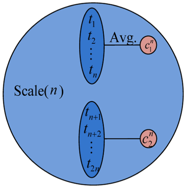
Schematic illustration of the coarse-grained time series for scale n.

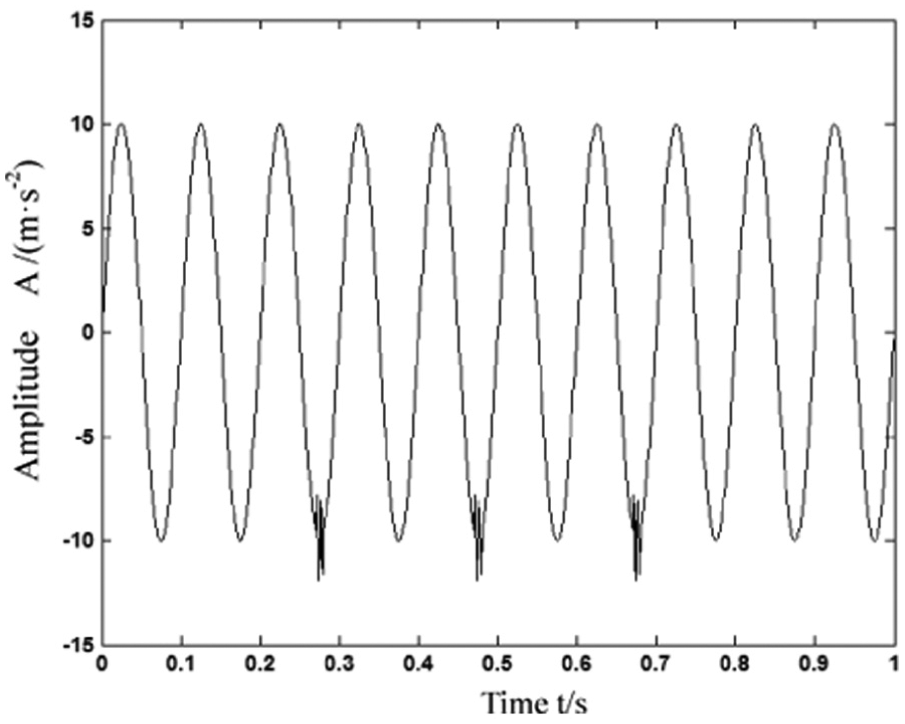
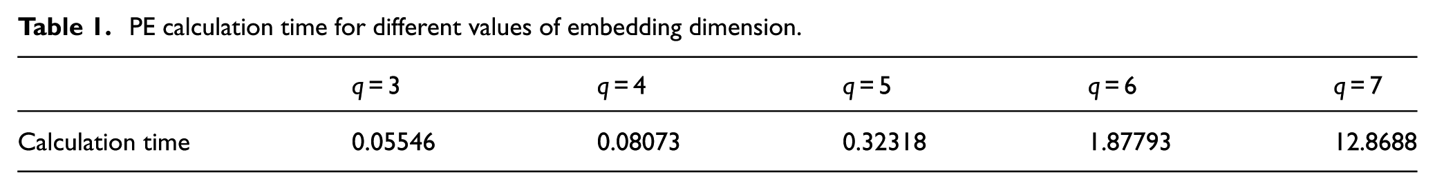
PE can be estimated for each coarse-grained series. ¹¹ PE is the function of l. The process of calculating PE is related to the value of embedding dimension q and time delay t. The embedding dimension q is usually between 3 and 7. If q is set to 1 or 2, the reconstruction vector will contain too few states for the algorithm to operate effectively and the algorithm will lose the ability of dynamic mutation detection in signals; if q is too large, the reconstruction of phase space will uniform time series, which will take too much time computing and the subtle changes of time sequence will not be reflected. As can be seen in Table 1, when q is 7, the time delay t causes less influence on calculation of time sequences. As shown in Figure 4, the time delay t has a small impact in PE of Gauss white noise signals. So, upon comprehensive consideration, this article takes q as 6 and t as 1 (Figure 6).

Table 1.

PE calculation time for different values of embedding dimension.

	q = 3	q = 4	q = 5	q = 6	q = 7
Calculation time	0.05546	0.08073	0.32318	1.87793	12.8688

Figure 6.

PE of Gauss white noise signals for different time delays.

ELM method

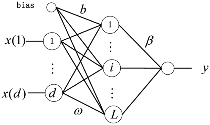
ELM is a new learning algorithm for unified single-hidden-layer feed forward neural networks (SLFNs). Its salient feature is that the input weights and hidden biases are randomly chosen and the output weights of SLFNs are determined analytically. The purpose of ELM was to render the training error and output weights as small as possible. Consequently, ELM tends to have better generalization performance and much faster learning speeds than traditional artificial neural network. Figure 7 shows the structure of the ELM network.

Figure 7.

Structure of the ELM network.

The output y with L hidden nodes can be defined as follows

$$y={\displaystyle \sum _{i=1}^L{\beta }_i{g}_i(X)}={\displaystyle \sum _{i=1}^L{\beta }_{i}G({\omega }_i,b_i,X)}=H\beta$$

(4)

Here, X indicates the input sample and $({\omega }_i,b_i)$ indicates the randomly generalized input parameters; X, ${\omega }_i\in R^d$ and $g_i$ denote the output of the ith hidden node output function $G({\omega }_i,b_i,X)$ ; H and $\beta$ represent the hidden layer output matrix and the output weight matrix, respectively. For N distinct samples $(x_j,t_j),j=1,\dots ,N$ , equation (1) can be written as follows

$$H\beta =T$$

(5)

Here

$$H=\left[\begin{array}{c}{h}_1\\ ⋮\\ h_N\end{array}\right]=\left[\begin{array}{c}{h}_{(x_1)}\\ ⋮\\ h_{(x_N)}\end{array}\right]={\left[\begin{array}{ccc}G({\omega }_1,b_1,x_1)& \cdots & G({\omega }_L,b_L,x_1)\\ ⋮& \cdots & ⋮\\ G({\omega }_1,b_1,x_N)& & G({\omega }_L,b_L,x_N)\end{array}\right]}_{N\times L}$$

(6)

$$\beta ={\left[\begin{array}{c}{\beta }_1\hfill \\ \multicolumn{1}{c}{⋮}\\ \multicolumn{1}{c}{{\beta }_L}\end{array}\right]}_{L\times 1}\mathrm{and}T={\left[\begin{array}{c}{t}_1\hfill \\ \multicolumn{1}{c}{⋮}\\ \multicolumn{1}{c}{t_N}\end{array}\right]}_{N\times 1}$$

(7)

Here, T represents the target matrix.

Because the input weights of its hidden neurons $({\omega }_i,b_i)$ would be generated randomly instead of tuned, the only parameter that must be calculated in the ELM is the output weight matrix $\beta$ , which can be easily acquired through least squares estimate (LSE)

$$\beta =H\prime T$$

(8)

Here, $H\prime$ is the Moore–Penrose generalized inverse of matrix H, which can be determined through orthogonal projection. ¹²

A flowchart of this proposed method for railway rolling bearing fault diagnosis using multi-scale IMF PE and ELM classifier was built based on the algorithm elements described above and is shown in Figure 8. As shown in the flowchart, the raw vibration signal is denoised by WD, EEMD is used to decompose the denoised signal into a set of IMFs, and the multi-scale IMF PE is calculated. Finally, the ELM is used for classification of the feature parameters.

Figure 8.

Flow chart of the novel intelligent fault diagnosis model.

Experimental results

Experimental setup

The experiments were performed on a SpectraQuest, Inc. fault simulator capable of simulating faults in various machine parts, such as the gearbox, shaft misalignment, and rolling element bearing. The experimental setup is shown in Figure 9. The simulation rig included one gearbox, a 3 hp motor and a magnetic brake. The simulator is driven by the 3 hp motor, and the motor rotating speed is directly controlled by a frequency converter. The load is provided by the magnetic brake and can be adjusted by a brake controller. Vibration signals are collected at a sampling frequency of 12 kHz for three different conditions under a given motor loading: (1) normal, (2) inner race fault, and (3) rolling element fault. The bearings are shown in Figure 10.

Figure 9.

Experimental setup for bearing fault diagnosis.

Figure 10.

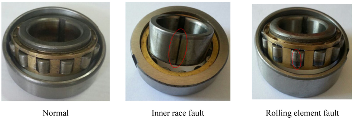
State of bearing.

Application

To evaluate the effectiveness of the extracted features in the recognition of different fault categories, the proposed approach was applied to the vibration signal with different fault categories. In this subsection, three vibration signal sets corresponding to normal condition, inner-race fault condition, and rolling element fault condition were acquired using the same data collection device. The sampling frequency was set to 12 kHz, and there were 4096 data points per sample. All these parameters were chosen by sampling theorem to ensure both accuracy and efficiency of the signal acquisition.

Figure 11 shows the railway rolling bearing acceleration vibration signals in three states, bearings in the normal state, bearings with inner race faults, and bearings with rolling element faults. The characteristics of the railway rolling bearing running states were buried in a great deal of noise. It was not possible to directly distinguish them by the time domain signals, because the differences among them are very subtle. Then each kind of the rolling bearing vibration signal is de-noised by WD. As shown in Figure 12, some background noise has been removed and SNR was improved after the WD filtration. EEMD is applied to decompose the de-noised signals to IMFs. Figure 13 shows the outcome when EEMD is introduced. Because the first five IMFs had almost all energy of the signal, other residual IMFs were omitted to guarantee the efficiency of the method. The energy distributions of EEMD indicated a clear distinction between the normal and defective rolling bearings. There were obvious periodic envelope features in the signals of defective bearing, but envelopes associated with normal bearing signals had no conspicuous periodicity.

Figure 11.

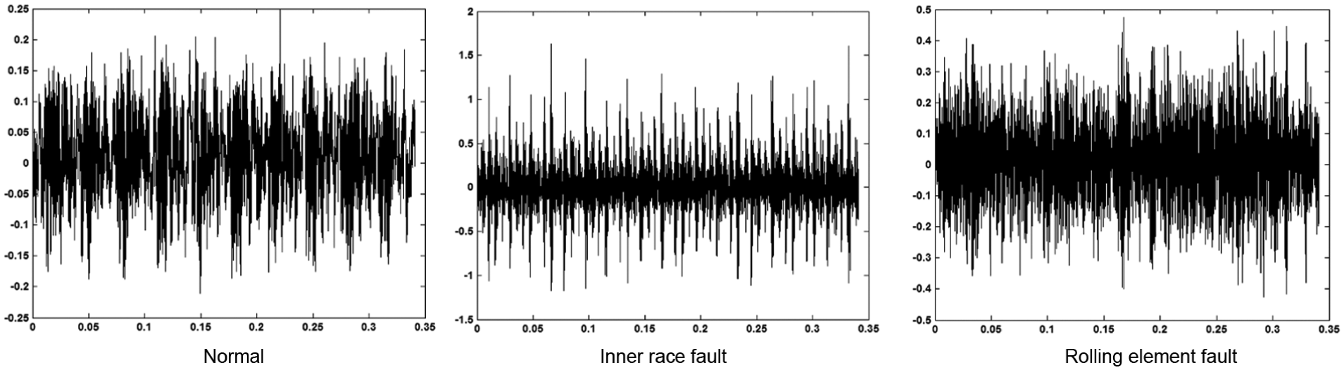
Time domain signal.

Figure 12.

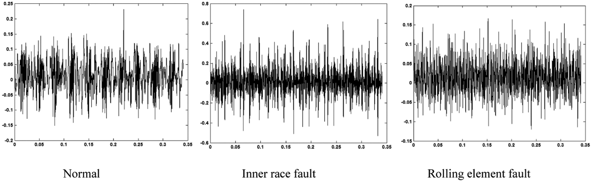
Denoised signal.

Figure 13.

Signal decomposed into five IMFs by EEMD.

When the rolling bearing conditions changed, the energy distribution of IMFs of EEMD changed as well; hence, the IMFs can be processed with time–frequency domain feature extraction for railway rolling bearing damage detection. According to the signal characteristics of the rolling bearing experiments in this article, the first five IMFs decomposed by EEMD are taken into consideration. Because 10 components already had the most energy of any components in the signal, these 10 energy features were extracted and have been transmitted to ELM as input.

Figure 14 shows the multi-scale IMF PE. A total of 20 experimental data sets were obtained for each operational condition, and 10 samples of every class were used to train the ELM classifier. After training, all samples, training, and testing data, were used to verify the accuracy of the output of ELM classifier for railway rolling bearing fault diagnosis. The purpose of the classification is to assign an input pattern to one of the three classes concerned and represented by the classification labels described in Table 2.

Figure 14.

Multi-scale time frequency permutation entropy.

Table 2.

Label of vibration signals of different kinds of rolling bearings.

Number of training data	Number of testing data	Rolling bearing type	Label of classification
10	20	Normal	1
10	20	Inner race fault	2
10	20	Rolling element fault	3

The output results of recognition are shown in Figures 15 and 16. As shown in Figure 15, the SVM classifier classified one sample wrong in that one normal condition was misjudged as inner fault condition. The testing results of elm are shown in Figure 16. As shown in Figure 16, there were three clearly different classifications, representing three different types of signals. After the comparison of the classification results and preset bearing conditions, the proposed intelligent approach was shown to have a high classification correct rate, approaching 100%.

Figure 15.

Testing results of SVM.

Figure 16.

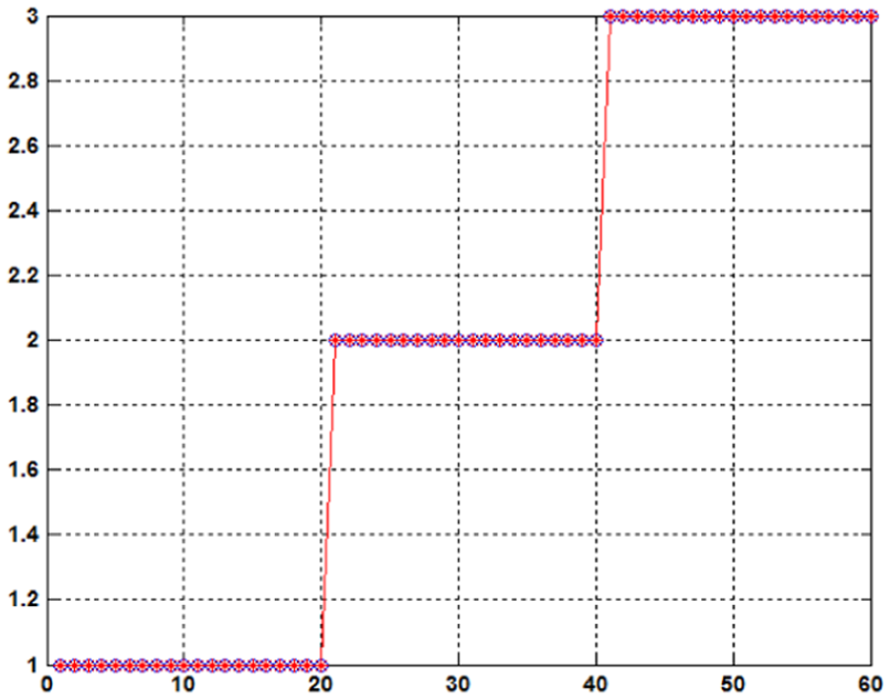
Testing results of ELM.

Conclusion

A new intelligent approach to the diagnosis of bearing faults using multi-scale IMF PE and ELM classifier combination is put forward in this article. In order to derive more fault information, multidimensional features from the time–frequency domains were extracted to reflect the bearing conditions from different angles. Fault samples of multi-scale IMF PE here served ELM input parameters to realize intelligent fault diagnosis. The results from experimental vibration signals with normal and fault bearings showed that the method of diagnosis proposed here could identify different working conditions of the railway rolling bearing status accurately and effectively.