
Abstract
This study improves upon the traditional polynomial detrending method in order to correct the vibration acceleration signals with inconsistent initial velocity and displacement more rationally and efficiently. When numerical integration of recorded acceleration signals using assumed initial velocity and displacement values (which are generally inconsistent with real values) is performed, baseline shift or drift phenomenon can arise in velocity and displacement curves obtained. Baseline correction must be performed if an inconsistent acceleration signal is to be used in dynamic analyses. Polynomial detrending is generally used to remove unreasonable trends in time series, but the consistency among acceleration, velocity, and displacement has not received sufficient attention. The traditional polynomial detrending method is improved by purposefully removing the shifted trends in velocity and displacement. Two inconsistent vibration signals are selected to be corrected using both the traditional method and the improved method. It was found that the traditional method does not give a satisfactory correction result, but the improved method can correct the signal to be consistent. The improved detrending method is effective in making vibration signals have consistent acceleration, velocity, and displacement.
Introduction
Vibration signals are generally measured or recorded using accelerographs, 1 and the corresponding time history data of velocity and displacement are obtained by taking the numerical integral of the recorded acceleration data. 2 To perform numerical integrations of acceleration, the initial values of velocity and displacement must be known. However, these values are difficult to obtain precisely; therefore, assumed initial values (usually, 0) are always adopted for performing the integrations. In most cases, the assumed initial values of velocity and displacement are inconsistent with real values, resulting in the phenomenon of baseline shift or drift of the velocity and displacement data (i.e. the baseline of a velocity or displacement curve shifts away from the time axis). In this study, this kind of vibration signal is termed “inconsistent.” The shifted or drifted data are irrational and not suited to be used for evaluating vibration amplitude or as input excitations. It is easy to eliminate the shift or drift trends from the velocity or displacement data individually, which is sufficient to provide proper values for the vibration amplitude although the acceleration data remain inconsistent. Using inconsistent signal as input acceleration excitations or boundary conditions for dynamic analysis can lead to incorrect results. A baseline correction needs to be conducted to ensure the velocity and displacement data obtained from acceleration data do not shift or drift away from the baseline. Polynomial detrending is one of most frequently used approaches for removing illegal trends in a time series. However, detrending operations are usually performed individually on acceleration, velocity, or displacement, without considering any interrelational consistency. This omission may cause the failure to correct acceleration data into having consistent and rational velocity and displacement after two integrations.
Incomplete acceleration records are the main source of inconsistent vibration signals, for example, truncated signals 3 or specially processed signals. 4 The precise starting and finishing instants of a vibration cannot generally be identified, and therefore, most recorded vibrational signals are incomplete records. Hence, a zero baseline correction is always needed for strong-motion data.5,6
For correcting inconsistent vibration signals, the most widely used solution is to remove the parabolic or polynomial trend from acceleration data or to apply a high-pass filter to them.5,7–10 However, these methods, which pay inadequate attention to velocity and displacement, cannot give satisfactory results if the baseline of displacement drifts heavily. Pecknold and Riddell 3 suggested adding a prefix acceleration impulse to make the records compatible, and Chiu 11 proposed a simpler form of the prefix impulse. Nevertheless, the amplitude of the additional prefix impulse is too large if the signal is significantly incompatible. Modern Global Positioning System (GPS) techniques12,13 are also used to correct baseline shift (or drift) according to recorded co-seismic displacement which prove to be more reliable and efficient; however, the GPS data of many old earthquakes may be not available.
This study theoretically explains the reason for the baseline shift (or drift) caused by inconsistent initial velocity or displacement. It also proposes approaches for estimating the real initial velocity or displacement. Two indicators are proposed for identifying the degree of baseline shift or drift and evaluating the correction results. The polynomial detrending method is improved and generalized to correct inconsistent vibration signals more effectively. Examples are provided to illustrate the efficiency of the improved baseline correction method over the traditional one.
Before any further discussion, the following preconditions need to be declared:
This study is concerned about the baseline shift or drift of velocity and displacement retrieved from acceleration data.
The acceleration data represent reciprocating motions starting at the static state, and thus, there is no baseline drift in reality.
The acceleration data are preprocessed, so that there is no noise interference.
Inconsistent signal
Simple demonstration
Denoting the acceleration, velocity, and displacement of a certain signal as


where t is the current time,
As mentioned above, the real initial velocity


where
The error between the pseudo results of velocity and displacement, and real-life results can then be obtained based on equations (1)–(4)

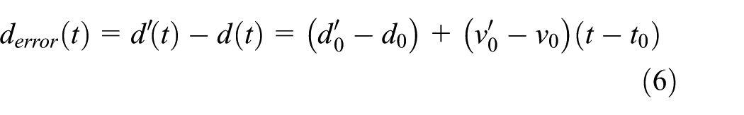
Equations (5) and (6) mean that the inconsistency between the assumed initial velocity and displacement, and real-life data, can lead to a constant error trend in the velocity and a linear error trend in the displacement. This can be demonstrated visually using harmonic waves. If the real displacement is

A simple demonstration of the phenomenon of baseline drift (The velocity and displacement curves are obtained by numerical integration of acceleration assuming
Estimation of initial velocity and displacement
According to equations (5) and (6), the inconsistent trends in velocity and displacement can be fitted by these polynomials, respectively

where
Because the order of error fitting polynomials
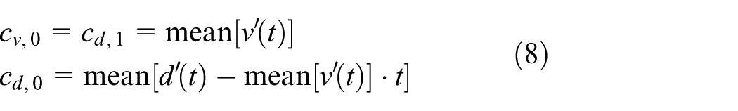
where “mean” stands for the operator used to obtain the average value of a signal

where
Then, the real values of initial velocity


Sometimes, the velocity and displacement values at a certain time may be known. For instance, earthquake signals should end with zero velocity and zero displacement since earthquakes ultimately stop. In this case, if the known velocity and displacement values at time

The real values of initial velocity

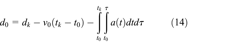
Using the initial values obtained from equations (10) and (11) or equations (13) and (14) in the numerical integration, the baseline shift or drift of inconsistent signals can be avoided; this forms the simplest baseline correction method. However, this method is only suitable for the evaluation of vibration amplitude signals. As mentioned in the introduction, because the acceleration signal itself remains unchanged, it is inadequate tackling the case of structural dynamic analysis using the inconsistent signal as an input excitation.3,14 Usually, the dynamic analysis of a structure begins with a static state, that is, the initial velocity and displacement are zero at the starting time. If the input excitation is inconsistent with the convention of
Baseline correction
Baseline drift indicators
For the phenomenon of baseline shift or drift caused by the inconsistency of initial conditions of numerical integration, an indicator termed the baseline drifting ratio
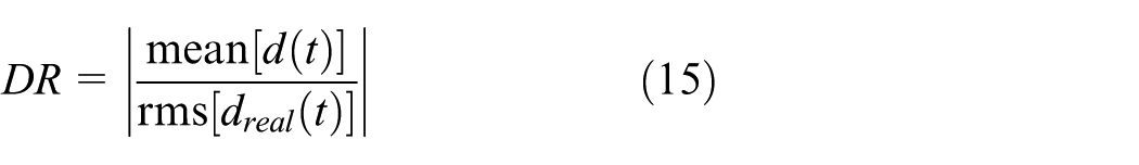
where

According to equation (15), the range of the baseline drifting ratio DR is

To describe the relationship between the degree of baseline drifting and DR visually, a series of displacement time history curves are drawn in Figure 2. It is suggested that a satisfactory baseline correction should make the final

Displacement curves with different degrees of baseline drift.
The displacement curve can be corrected directly by subtracting the linear trend from it according to equation (6), but this has no influence on the acceleration since the linear trend would vanish after two successive differential operations (because acceleration is the second derivative of displacement). This means that theoretically, accurate baseline correction is unrealizable for inconsistent signals; hence, only approximation methods can be used. However, approximation methods may introduce unpredictable high-order polynomial trends that could invalidate the drifting ratio DR for judging the baseline drifting degree (Figure 3). Therefore, a new indicator termed the amplitude ratio


Displacement curves with the same drifting ratio.
Curves in Figure 3 show that the closer AR is to 1, the more satisfactory the results of baseline correction under a constant drifting ratio DR. It is suggested that the amplitude ratio AR should also be controlled such that
Besides the two indicators DR and AR, the correlation coefficient between
Improved detrending algorithm for baseline correction
The most widely used algorithm for baseline correction (referred to as the traditional detrending algorithm in this study) removes the polynomial trend from an acceleration time history curve. It has been adopted by the well-known ground motion signal processing software SeismoSignal 15 for adjusting the baselines of strong-motion data. However, the traditional detrending algorithm only involves removing polynomial trends in the acceleration data without paying any attention to the velocity and displacement. Therefore, it sometimes cannot bring about a satisfactory result, especially for signals whose envelope lines do not have attenuate endings. Besides, the traditional detrending algorithm needs several trial computations to confirm the most suitable order of the fitting polynomial, and a relatively high-order fitting polynomial may over-correct the signal to shift or drift in the opposite direction. To make the method more effective, an improved method (referred to as the modified detrending algorithm in this study) is proposed in this section following the idea of polynomial detrending.
Before further discussion, some notation needs to be declared explicitly:


The traditional algorithm for baseline correction can be described as follows. An Mth order polynomial

Equation (22) shows that the processing object in the traditional method is acceleration, but the phenomenon of baseline drifting mainly occurs in velocity and displacement. This leads to the inefficacy of the traditional method when dealing with a marked drifting phenomenon. Therefore, inspired by Graizer’s 16 method and Iwan et al.’s 17 method, an improved baseline correction method whose processing objects are velocity and displacement is proposed in this study on the basis of polynomial detrending approaches. Shown below are the two steps of the modified detrending algorithm for baseline correction:
Step 1. Integrate the acceleration

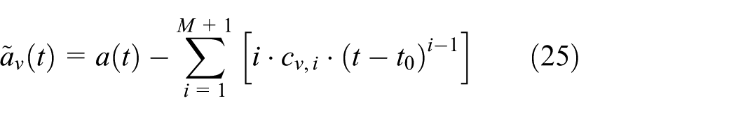
According to the differential relationship between acceleration and velocity, the corresponding corrective time series

When the coefficients
Step 2. Integrate the corrected acceleration

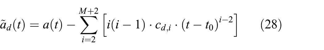
According to the differential relationship between acceleration and displacement, the corresponding corrective time series

When the coefficients
In conclusion, the final corrected acceleration can be expressed as

The baseline correction procedure conducted by equation (29) is referred to as Mth order correction because the corrective time series for acceleration is an Mth order polynomial. The selection of the corrective order is mainly dependent on the degree of baseline drifting: the more severely the baseline drifts, the higher the selected order should be. However, setting the corrective order to a very large value (empirically
Baseline correction examples
In this section, two examples are provided from different sources to illustrate the improved detrending algorithm proposed in this study for baseline correction of vibration signals.
Example I: a truncated ground motion record
The first example is correction of a manually truncated ground motion record. The original record is derived from the Pacific Earthquake Engineering Research Center (PEER) Next Generation Attenuation (NGA) ground motion database and is a site record of the CHY039 strong-motion station (23.5207°North, 120.3440°East) during the Chi-Chi Earthquake in 1999. The NGA number of the record is 2711, and the east-west component (named “NGA-2711-E”) is chosen as the processing object in this section. The time history curve of the original data is shown in Figure 4, where the velocity and displacement are obtained by integrating the acceleration signal with the assumed initial condition

Original time history curve of NGA-2711-E (the shaded area indicates the Arias intensity; vertical lines show the cut-off locations).
Because the original record is fairly long and may be time-consuming when selected as the ground motion input for dynamic analysis of tall building structures, it is truncated owing to the accumulated Arias
18
intensity of the original acceleration record. As a result, the original data between 10 and 63 s are kept corresponding to an Arias intensity between 1% and 99%. Then, if the assumed initial conditions

Truncated time history curve of NGA-2711-E (the gray line is the displacement obtained using the estimated initial velocity and displacement).
The corrected time series using the traditional detrending algorithm are shown in Figure 6, from which we can see that the resulting displacement curves are obviously different from the original displacement shown in Figure 1 (or the gray lines in Figure 6), while the drifting ratio and amplitude ratio are relatively large (distinctly larger than the suggested indices:

Baseline correction of truncated NGA-2711-E using the traditional detrending algorithm (thin gray lines are the displacement obtained from the original record).
Figure 7 shows the corrected results obtained by the modified detrending algorithm, and the corrective orders are selected as

Baseline correction of truncated NGA-2711-E using the modified detrending algorithm (thin gray lines are the displacements obtained from the original record).
Example II: a floor vibration record induced by machines
The second example involves correcting a record of periodic ground motion induced by mechanical equipment. Because the vibration source is periodic, the displacement should be reciprocating. However, after integrating the acceleration record using assumed initial conditions

Original time history curve of SM001.
In order to evaluate the vibration amplitude, we need more rational displacement results. When equations (10) and (11) are adopted for estimating initial conditions, the drifting trend vanishes (the gray line in Figure 8) after numerical integration using the estimated initial values of velocity and displacement. The amplitude of the time series is then more credible for evaluating the vibration. However, we also need to use the recorded acceleration signal as the input excitation source to analyze the dynamic response of the plant where the equipment is located. Hence, the record must be corrected to be compatible with assumed initial conditions. Similar to Example I, two different baseline correction algorithms are tried out for adjusting the record, and the corresponding results are shown in Figures 9 and 10, respectively. From these figures, similar conclusions to those in Example I can be drawn: the traditional detrending algorithm is a hypercorrection with respect to the original record, in a sense, and the corrected curves drift more significantly than the original ones (Figure 9). Meanwhile, the improved algorithm proposed in this study can effectively control the drifting phenomenon in displacement and provide a rational input acceleration excitation for dynamic analysis.

Baseline correction of SM001 using the traditional detrending algorithm (thin gray lines are the detrended displacements).

Baseline correction of SM001 using the improved detrending algorithm (thin gray lines are the detrended displacements).
Conclusion
Initial values of velocity and displacement are important in the process of integrating acceleration data into velocity and displacement. Inconsistent initial integration conditions may result in baseline drifting and even errors in response analysis of long-period structures. The incompatible baseline drifting phenomenon is usually reflected in the integrated velocity or displacement curves, and the traditional detrending algorithm used for baseline correction does not address these quantities. This makes the traditional detrending algorithm unsuitable for use with heavily drifted signals. In this study, the traditional detrending algorithm was improved to take velocity and displacement into account in order to correct inconsistent vibration signals. The proposed algorithm has been successfully applied to baseline correction of a truncated strong-motion record and a mechanical vibration record. Comparisons between the traditional detrending algorithm and the two target-based algorithms indicate that the proposed algorithms are more suitable and effective for adjusting inconsistent vibration signals into rational ones.
Footnotes
Academic Editor: Balla Prasad
Declaration of conflicting interests
The author(s) declared no potential conflicts of interest with respect to the research, authorship, and/or publication of this article.
Funding
The author(s) disclosed receipt of the following financial support for the research, authorship, and/or publication of this article: This study was supported by the National Natural Science Foundation of China (Grant Nos 51308418 and 51478356), the Shanghai Committee of Science and Technology (Grant No. 10DZ2252000), and the Sichuan Department of Science and Technology (Grant No. 2016JZ0009).