
Abstract
In practical engineering, reliability analysis of products plays an important role in assessing the corresponding remaining life. Products often have more than one failure mechanism, which means reliability should be evaluated by two or more performance characteristics. To resolve the above problem, based on the degradation values distribution method utilization, copula functions as the link functions of their marginal distributions are introduced in this study. The performance characteristics are also considered the dependent as well as independent to make a comparison. Moreover, a framework for reliability assessment of products with the multiple performance degradation is developed. Finally, the proposed methodology and model is validated effectively by the fatigue cracks data from the literature. From the results, we can see that the proposed model is more accurate.
Keywords
Introduction
With the development of science and technology, the manufacturing and management level of products has been increasing significantly. It makes that the higher reliability and the longer lifetime of products are needed. Product lifetime data are necessary for reliability analysis. However, it is usually not easy to obtain enough lifetime data in short time. In this situation, the degradation-based reliability modeling has been widely recognized as an alternative approach to solve reliability evaluation issues, such as limited data, long lifetime, and no failure data. In fact, the failures of most products are caused by performance degradation, such as abrasion of mechanical components, aging of the insulating materials, and crack growth in metal materials. Compared with the traditional lifetime data, more useful information about the accumulation of damage can be found from the degradation data. Based on the degradation information, the effective products reliability evaluation can be made.
Since the 1970s, many researches on reliability modeling methodologies using degradation data have been made. Lu and Meeker 1 proposed a regression model of degradation data to estimate a time-to-failure distribution. The time-to-failure distribution and confidence intervals were estimated by Monte Carlo simulation and bootstrap methods. Park and Padgett 2 used a gamma process to model degradation of products and incorporated an accelerated test variable. Tsai et al. 3 developed a model based on Wiener process with random drift. It was applied to solve some practical problems. Wang et al. 4 proposed a degradation model based on Wiener process which was applied in hybrid deteriorating systems successfully. Bagdonavicius and Nikulin 5 proposed a degradation model based on gamma process which included possibly time-dependent covariates. A degradation model based on inverse Gaussian process (IGP) was proposed by Wang and Xu 6 . Peng et al. 7 developed a Bayesian inference method to estimate the parameters which was applied in his model based on IGP. In addition, many authors make a lot of researches about reliability modeling for competing failure mode by jointly considering the degradation process and associated catastrophic failure.8–10 Wang and Coit 11 made the research about the degradation model with random or uncertain failure threshold.
These studies make valuable contributions to the reliability modeling using degradation data. However, most of these researches are based on the assumption that there is only one performance characteristic. In fact, products may have multiple degradation. It means multiple degradation paths for products failure should be considered simultaneously.
For multiple degradation processes, Crk 12 supposed that the system failure mechanism is mutual independent and proposed a method to estimate the reliability of system by monitoring each performance degradation. Pan and Balakrishnan 13 developed a bivariate degradation model based on gamma process and bivariate Birnbaum–Saunders distribution. Sari et al. 14 used the copula function to develop a two-stage model for bivariate processes. They also took the experiment data from light-emitting diode (LED) lighting systems as an example to illustrate the application of the proposed model. Wang and Coit 15 proposed a degradation modeling and analysis approach for reliability prediction considering multiple degradation measures. Hao and Su 16 make the research about the bivariate correlated degradation model based on random effect nonlinear diffusion process and copula functions. Beside these works, a lot of researches about multiple failure modes have been given by Huang and Askin, 17 Bagdonavicius et al.,18,19 Belmansour and Nourelfath, 20 Meng and colleagues21–24, and Sklar 25 and Zhu.26,27
However, previous researches only focus on the independency of performance characteristics or multivariate normal distribution, which are not usually suitable in many practical situations. Many authors introduced the reliability modeling based on the stochastic process, which is more accurate theoretically. However, it is difficult to fit degradation data with stochastic process when degradation path makes a great difference between samples. In this case, the method based on degradation values distribution is a relative better choice. In this study, we utilize the degradation values distribution method to describe degradation process, which is different from the previous multiple degradation processes researches. Then, the relation of the performance characteristics is described by a copula function. The parameters of the copula function are estimated by Bayesian Markov chain Monte Carlo (MCMC) method.
The organization of this study is as follows. In section “Reliability modeling of univariate degradation data based on degradation values distribution,” the reliability model of single performance measure based on degradation values distribution is introduced. In section “Reliability modeling of multiple degradation data,” the multiple degradation model using copula functions is proposed. In section “Parameter estimation,” the method of inference for the model parameters is introduced. A numerical example about fatigue cracks growth is given in section “Numerical example.” Section “Concluding remarks” concludes the study.
Reliability modeling of univariate degradation data based on degradation values distribution
Analysis of the reliability modeling based on degradation values distribution
In practice, the degradation performance characteristics of many products can be treated as a stochastic variable in practice. It means that the degradation data of each sample is random at the same measurement moment. Therefore, the degradation process using degradation values distribution method can be described. With the development of the degradation process theory, the degradation values distribution curve including the failure threshold is more and more close, which makes the reliability of products performance less. The above process is shown in Figure 1. Therefore, if an accurate reliability model of the degradation values distribution at each measurement moment is put forward, the reliability of the products can be assessed exactly. In this study, the degradation values distribution curve at each measurement moment is obtained. Then, the parameters of the degradation values distribution curve are described as a time function to illustrate the degradation process of products.

Statistical analysis based on degradation values distribution.
The general assumptions in reliability modeling based on degradation values distribution are as follows:
The degradation values distribution of all samples at each measurement moment belong to the same distribution family.
The parameters of the distribution family changes over time and can be fitted by time function.
The failure threshold of the sample is a constant. When the degradation of the sample reaches the failure threshold first time, it will fail.
Reliability modeling based on degradation values distribution
Suppose in the degradation experiment, there are n units tested and m measurements for all the units are observed up to the termination time T. Define
In this study, the degradation values distribution type was selected by goodness-of-fit test. There are many degradation values distribution types proposed in the related research. We select normal distribution, logarithmic normal distribution, Weibull distribution, and gamma distribution as the alternative types in this study.
Assume that

So, the probability density function (PDF) of

and the cumulative distribution function (CDF) of

In the degradation process,

where
The marginal distribution function could be described as

where
If the failure threshold is

Reliability modeling of multiple degradation data
Compared with the assumption of the independent property in many studies, it is more accurate to consider the relation among multiple degradation paths in practical engineering. Assume that the multiple performance characteristics are dependent mutually and obtain an estimate of the joint distribution by a copula function. Copula function is used to connect marginal distributions so as to constitute a joint distribution. The multivariate dependency can be separated from the modeling of the marginal data. Sklar’s theorem
28
is the theoretical foundation of copula function. According to Sklar’s theorem, if H is a joint distribution function with continuous margins

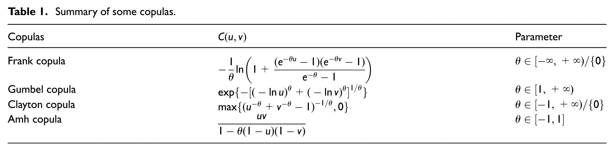
Some well-known copulas are listed in Table 1, in which u and v are marginal distributions.
Summary of some copulas.
Assume that a product has multiple degradation processes. These degradation processes can be expressed as

where
In this study, we assume that the product failure occurs if degradation process reaches its failure threshold, which is defined as
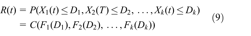
If the multiple performance characteristics are independent, the product reliability can be expressed simply as

Parameter estimation
In this section, the estimation of the model parameters is discussed. For products with multiple degradation characteristics, the reliability model not only has a lot of parameters but also is very complicated or even infeasible to be utilized in computation. Therefore, a method of two-stage procedure is proposed to reduce the computational difficulty. The process is that the marginal distribution is estimated first and then the copula parameter from jointly likelihood with marginal parameters estimated in the first stage is calculated.
Stage 1 (marginal parameters)
Each marginal distribution
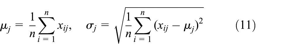
After substituting equation (11) into equation (4), we have

The type of the above function and the estimation of the parameters can be concluded by data fitting with curve fitting toolbox in MATLAB®.
Stage 2 (copula parameters)
We denote
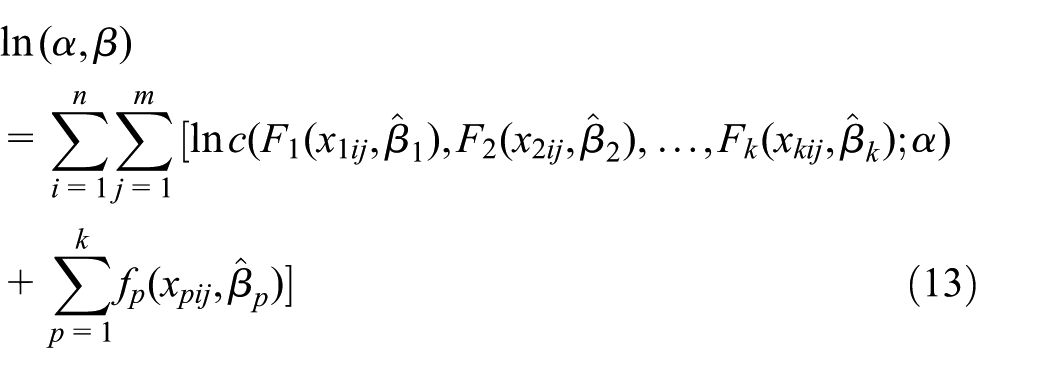
where
Because it is computationally difficult to work with the log-likelihood function, we estimate the copula parameters via Bayesian MCMC method. A sample from the posterior distribution based on a Markov chain can be generated through the MCMC method. Then, an accurate estimate of any desired feature of the posterior distribution can be gotten. In this study, the prior distributions of all the unknown parameters are assumed as non-informative. Furthermore, OpenBUGS 29 is used to achieve the Gibbs sampling and estimate the model parameters.
Numerical example
In this section, the model proposed in section “Reliability modeling of multiple degradation data” is illustrated. The fatigue crack data are used which are presented in Meeker and Escobar
29
and are listed in Table 2. In the original data, there are 21 samples which are measured every 0.01 million cycles from 0 to 0.09. The time unit is in million cycles. In this study, the first 20 samples are chosen and divided into two groups to represent two performance characteristics. Samples in the first group are defined as crack A and samples in the second group are defined as crack B. Therefore, crack A is treated as the first performance characteristic and crack B is the second performance characteristic, respectively. The product is considered to occur if the length of crack A is more than 1.6 in or the length of crack B is not less than 1.3 in, which means
Fatigue crack data taken from Meeker and Escobar. 29


The development of crack A length over time.

The development of crack B length over time.
In this section, the difference of the degradation data and the initial data is used for calculation.
Goodness-of-fit test
The goodness-of-fit test is applied to determine the type of each marginal distribution via Minitab. On the basis of degradation values distribution types proposed in the related researches, normal distribution, logarithmic normal distribution, Weibull distribution, and gamma distribution are selected as the alternative types of the marginal distribution. The goodness-of-fit tests of two groups are completed by Anderson-Darling. The results are shown in Table 3. Figure 4 shows the result of crack A with goodness-of-fit test in the measurement time 0.06. Figure 5 shows the result of crack B in the measurement time 0.05.
The result of goodness-of-fit test.

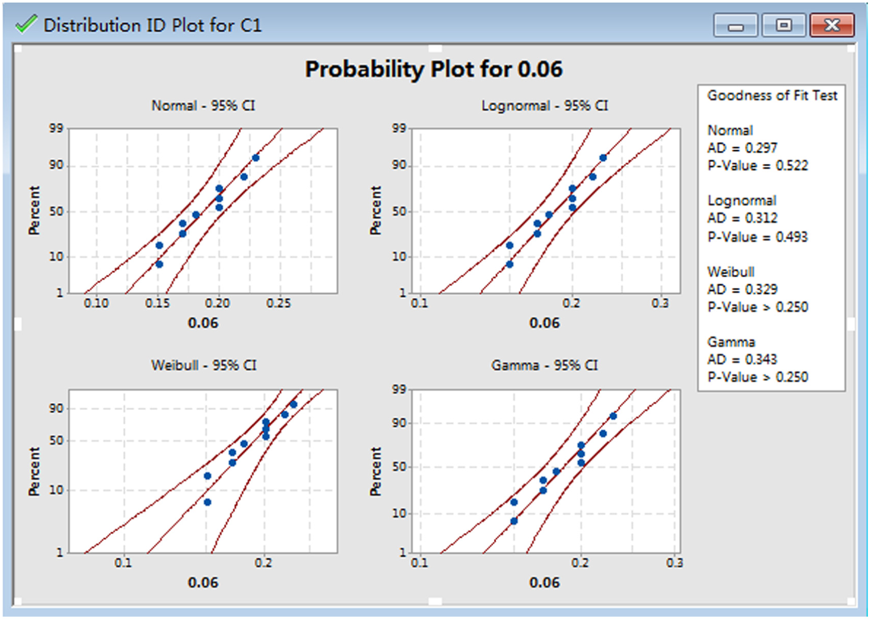
The result of crack A with goodness-of-fit test.

The result of crack B with goodness-of-fit test.
On the basis of the result of goodness-of-fit test, crack A follows normal distribution and crack B follows Weibull distribution.
Estimation of parameters
Stage 1
We can calculate the mean and standard deviation of both marginal distributions based on equation (11) over each 0.01 million cycles. The shape parameter and scale parameter of Weibull distribution can be calculated via 1-Stopt. The results are shown in Table 4. Based on equation (12) and the data in Table 4, the type of the time function and the estimates of the parameters can be determined via curve fitting toolbox in MATLAB.
Observations of the parameters of both marginal distributions.

Time function in equation (12) can be expressed in Table 5 based on Table 4.
Estimates of the parameters of marginal distribution.

Suppose the shape parameter in Weibull distribution is a constant because we find it has nothing to do with time in Figure 6 (m). Therefore, use the mean of the observations to represent it. Figure 6 shows the result of fitting data via curve fitting toolbox in MATLAB.

The result of fitting data.
Stage 2
Here, consider a copula function to describe the dependency between both marginal distributions. And select the Frank copula as a link function directly. Frank copula is a kind of Archimedean copulas and its structure is symmetrical. It can be used not only to describe the positive correlation between variables but also to describe the negative correlation relationship between variables. Its CDF


With the given estimates of marginal distribution in Stage 1, estimate the copula parameter
The estimates of copula parameter.

Reliability assessment
In this section, the reliability according to equations (6), (9), and (10) is estimated considering the cracks to be dependent and independent, respectively. Figure 7 shows the results of reliability assessment.
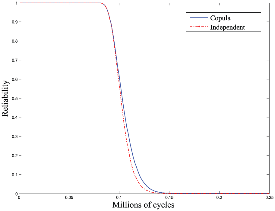
Comparison of the system reliability under both copula and independent assumptions.
From Figure 7, the copula reliability curve and independent reliability curve are overlapped at early age. The reason is that both of two performance characteristics are in good condition in the early time and they have little impact on each other. After the measurement 0.01 millions of cycles, the independent reliability curve tends to be slightly falling faster than copula reliability curve. It shows that there are mutual effects between multiple performance characteristics in the late stage of product degradation. Therefore, the reliability of products with multiple degradation processes may be underestimated with the assumption of independence. The reliability model considering the dependence between multiple degradation processes is more accurate.
Concluding remarks
In this study, a reliability model of products with multiple degradation processes is developed via the copula function. The method of degradation amount distribution is introduced to describe marginal degradation process first. A reliability model subject to dependent multiple degradation processes is proposed using copula functions. The parameters of the model are estimated by a two-stage procedure method considering its complexity. From the numerical example in section “Numerical example,” the performance of the proposed model is effective as the corresponding inferential method. The comparison of performance characteristics is made between independent and dependent. The results revealed that the system reliability tends to be higher than independent situation after early stage. Therefore, the proposed model is more accurate for the multiple degradation data.
Footnotes
Academic Editor: Yongming Liu
Declaration of conflicting interests
The author(s) declared no potential conflicts of interest with respect to the research, authorship, and/or publication of this article.
Funding
The author(s) disclosed receipt of the following financial support for the research, authorship, and/or publication of this article: This research was supported by the National Natural Science Foundation of China under contract No. 51505067.