Modeling and simulation of dynamical contact of asperities between flat rough surfaces

Abstract

Dynamic contact analysis on the level of surface asperities is a powerful means to study the wear behavior of surface and the physical contact properties of interface. This article established an analytical model of asperity contacts between nominal rough planes during sliding process based on the statistical contact analysis of rough surfaces. The analytical expression describes the mathematical relationship between the total number of asperity contacts and its main influencing factors including the nominal contact area, sliding distance, the spacing between two contact planes, and surface topographical parameters. A simulation model of dynamic contact of asperities on rough planes was established to rapidly calculate the number of asperity contacts during the sliding process. The comparison between the calculation results and simulation results of the number of asperity contacts obtained through multifactor and multilevel analysis verified the rationality of the analytical model.

Keywords

Dynamic contact of asperity statistical contact model mathematical model simulation model surface topography

Introduction

Since machining surfaces are composed of randomly distributed asperities with different heights, the contact of rough planes in movement will lead to the elastic or elastic–plastic dynamic contact of the asperities. Studies of rough surface contact were mainly focused on the features of the pure contact (static contact), including the contact area, deformation, and stress distribution of single asperity or multiple asperities under a certain external force. Relevant study methods included several theoretical modeling methods,¹ the numerical analysis methods,^2–4 and experimental study methods.^5,6 Current studies of surface dynamic contact were mainly focused on the stress–strain of asperities during the sliding contact process^7,8 and unstable friction (dynamic friction) caused by the changes in the micro-contact spacing during the surface sliding process.^9–11 The study of dynamic contact parameter of asperities on rough planes during sliding process, i.e. total number of asperity contact, was not reported. From the microscopic perspective, fatigue wear of sliding friction surfaces is the accumulated fatigue damage caused by repeated elastic contacts of asperities. Therefore, total number of asperity contact during sliding process is an important factor in microscopic fatigue wear of the surfaces. Moreover, because the current and heat of two contact surfaces is delivered through asperity contact, the dynamic contact parameter of asperities during sliding process can be used to analyze the dynamic contact resistance and thermal contact resistance of the two surfaces during the sliding movement. The study of dynamic contact parameter of rough surfaces can provide new research idea for modeling of the friction and wear behavior of contact surfaces and the physical contact properties of interface.

In order to establish the dynamic contact model of rough planes, it is necessary to obtain the rational model descriptions of rough surfaces. In the past decades, the modeling of the contact between rough surfaces was extensively studied. Due to the randomness and anisotropy of the surface topography, the theoretical modeling is very difficult. The classical statistical model for the analysis of the elastic andelastic–plastic hybrid contact between a rough surface and a smooth surface was proposed by Greenwood and Williamson (GW),¹ it is assumed that the rough surface is composed of hemispherical asperities with the same curvature radius, and that the height of hemispherical asperities follows the Gaussian distribution. In addition, it is also assumed that the deformations of different asperities are independent from each other during the asperity contact. The model was amended by Whitehouse and Archard¹² and Onions and Archard.¹³ With the development of surface topography measurement techniques and numerical analysis techniques, based on GW model, Bush et al.,¹⁴ Gibson,¹⁵ and McCool¹⁶ established a new elastic asperity contact model, in which the asperities were treated as elliptical paraboloids with randomly oriented elliptical contact areas. Kotwal and Bhushan¹⁷ established a statistical non-Gaussian surface contact model to enhance the application of the statistical contact model.

Majumdar and Bhushan^18,19 established a fractal contact model of rough surfaces, in which fractal geometrical parameters were used to describe the surface topography, and the uncertainty of topographical parameters was avoided. The development of the computer technology allows the digital treatment and computer simulation of the surface contour^20–22 to obtain the digital surface topography, in which the shape, size, and height distribution of the asperities can be arbitrarily designated to more accurately indicate the actual surface topography. Digital topography of different contact surfaces can also be used to analyze the surface asperity contacts and obtain the contact contours. Although statistical contact models, compared to other contact models, have some limitations and a certain deviation from real rough surfaces, a number of simple topographical parameters and simple mathematical expressions are adopted to predict the real contact area, contact load, and the parameters of other surface contact properties, and such prediction results have been proved by many theoretical and practical research.²³ Compared to other contact models, statistical contact models have theoretical and practical significances. Therefore, statistical contact models are still widely used in the surface micro-contact analysis of engineering machinery. In this article, based on the statistical contact theory, the asperity contact model of nominal rough planes was established. The rough surface asperity was approximated to the spherical body with the same curvature radius. Thus, the contact between two planes could be considered as the contact among a series of spherical bodies with different heights.

In this article, the dynamic contact model was established according to the following two steps. First, based on the statistical analysis theory, a surface asperity model was established to analyze the static elastic contact parameters of two rough planes, including the contact area and the number of the contacted asperities. Second, based on the fact that the transient contact parameter of rough planes was the same during sliding process, the dynamic contact model of orderly asperities was established to obtain the analytical expression of the number of asperity contacts through statistical integration.

To validate the dynamic contact model, a simulation model of the dynamic contact of asperities between rough planes was established in this article. In the simulation model, based on the established mathematical model of rough planes, the relative sliding process of surfaces was simulated, and the contact number of asperities during the sliding process was cumulatively calculated. The comparison results between the theoretical value and the simulated value of the number of asperity contacts verified the rationality of the theoretical analysis model.

Statistical contact modeling of nominally flat rough surfaces

The topography of nominally flat rough surfaces, as shown in Figure 1(a), is composed of a series of randomly distributed asperities. The surface topography can be characterized with a group of three-dimensional (3D) statistical parameters obtained through topography measurement. These 3D statistical parameters include the arithmetical mean µ of asperity height, the standard deviation σ of asperity height, the distribution function ψ(z) of asperity height (asperity height z is the distance from the top of an asperity to the reference plane), the mean radius R of asperities, the surface density D of asperities, and so on. As the elastic contact between rough surfaces occurs at the tips of the asperities on reference planes and the tip edge of the asperities is circular arc, the rough surfaces can be represented by an asperity model which is defined by a series of elastic spheroids, as shown in Figure 1(b). The radii of the spheroids are equal to the mean radius R of asperities on the rough surface, and the height of each spheroid is the same as the height of the corresponding asperity. The asperity model in Figure 1(b) will be used to analyze the elastic contact of nominally flat rough surfaces.

Figure 1.

Modeling of the topography of nominally flat rough surfaces: (a) actual rough surfaces and (b) the elastic asperity model of the rough surfaces.

When two flat rough surfaces are in the elastic contact, the contacts occur on part of the asperities on the surfaces, as shown in model I of Figure 2. The rough surfaces are constructed by the asperity model of Figure 1(b). The contact spots (the top view of model I) present the contact state of asperities, including the number of contact asperities and the contact area of each contact asperity. According to the statistical contact model proposed by Greenwood and Tripp,²⁴ the contact of two rough surfaces can be represented as the contact between a rigid plane and an equivalent rough surface, as shown in model II in Figure 2. The contact spots of model II are consistent with those of model I. The equivalent rough surface (the lower surface in model II) is defined with the composite standard deviation σ′ of asperity height and the composite mean radius R′ of asperities of the two rough surfaces in model I. σ′ and R′ are expressed by equations (1) and (2) as follows

σ' = \sqrt{σ_{1}^{2} + σ_{2}^{2}}

(1)

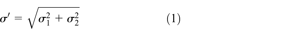
where σ₁ and σ₂ are the standard deviations of asperity height distribution of the two original rough surfaces

\frac{1}{R'} = \frac{1}{R_{1}} + \frac{1}{R_{2}}

(2)

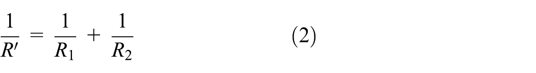
where R₁ and R₂ are the mean radii of asperities of the two original rough surfaces. Let n be the number of asperities and ψ(z) be the distribution function of asperity height; then the number of contact asperities m and the real contact area A of model II can be obtained by equations (3) and (4) as described by GW¹

m = n \int_{h}^{\infty} ψ (z) dz

(3)

A = m π R' (z - h) = n π R' \int_{h}^{\infty} (z - h) ψ (z) dz

(4)

where h is the distance between the reference planes.

Figure 2.

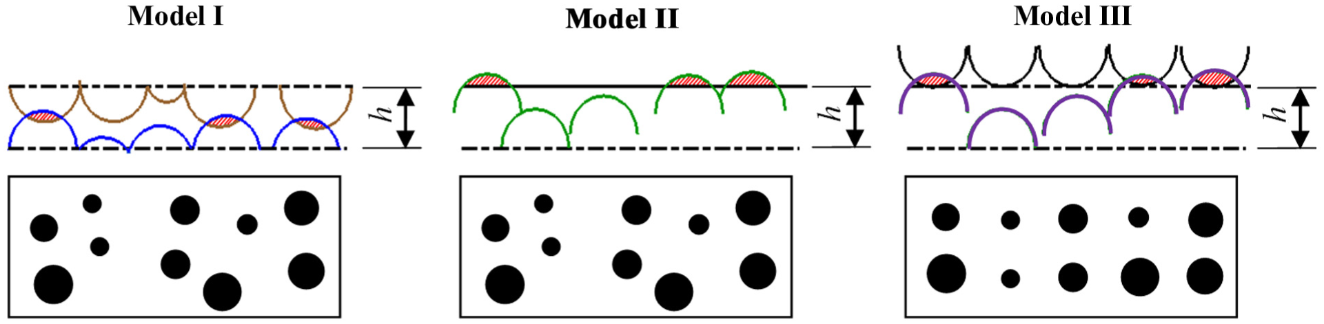
Equivalent transformation of the static elastic contact of nominally flat rough surfaces: model I, elastic contact of two rough surfaces; model II, elastic contact of a rigid plane and the equivalent rough surface; model III, equivalent contact model of model II with ordered asperities. The asperity contact states of model I, model II, and model III are the same.

The upper rigid plane of model II can be further equivalently represented as a rigid flat surface with uniform and orderly asperities, as shown as the upper surface of model III, which is based on the following conditions: (a) the height of the asperities is uniform, and their top is leveled with the original rigid plane in model II and (b) the radius and surface density of the asperities are consistent with the asperities of the lower surface of model II. The two upper surfaces of model II and model III have the same contact effect.

The asperities on the lower surface of model II can also be orderly distributed in lines without changing the topography parameters of the surface, which brings about the lower surface of model III. This equivalent transformation guarantees the contact parameters of model II and model III are in consistency.

As shown in Figure 2, the number of contact asperities (m) and the contact area of each contact asperity (also the total contact area A) of model III and model II are the same, although the contact spots of model III are orderly distributed, and those of model II is stochastic. The three models in Figure 2 have the equivalent contact since they present identical contact states of asperities. The orderliness of model III makes it efficient to analyze the dynamic contact of two rough surfaces.

Dynamic contact modeling of nominally flat rough surfaces for calculation of number of asperity contacts during sliding process

As shown in Figure 3, when a nominally flat rough surface slides on another nominally flat rough surface, the asperities on the interface contact each other randomly due to the stochastic surface topography. The contact state of asperities (shown as contact spots) on the contact interface at every moment during sliding can be treated as the static elastic contact of nominally flat rough surfaces represented as the models in Figure 2. Therefore, the contact parameters (m, A) at every moment during sliding can be calculated by equations (3) and (4). If the two nominally flat rough surfaces are machined uniformly and the parameters of topography are consistent throughout the surfaces, the contact parameters (m, A) calculated by equations (3) and (4) for every instant remain constant during sliding. That is to say, the contact of asperities for every instant during sliding process can be evaluated by the static elastic contact model III with the identical surface topography parameters. Thus, when a sliding rough surface with the nominal area S slides on a fixed rough surface for the distance l, as shown in Figure 3, the dynamic contacts of asperities during sliding process can be described by a Model III when its upper rigid surface (with nominal area S) slides on the lower surface for the distance l, as shown in Figure 4.

Figure 3.

Relative sliding of two nominally flat rough surfaces under elastic contact.

Figure 4.

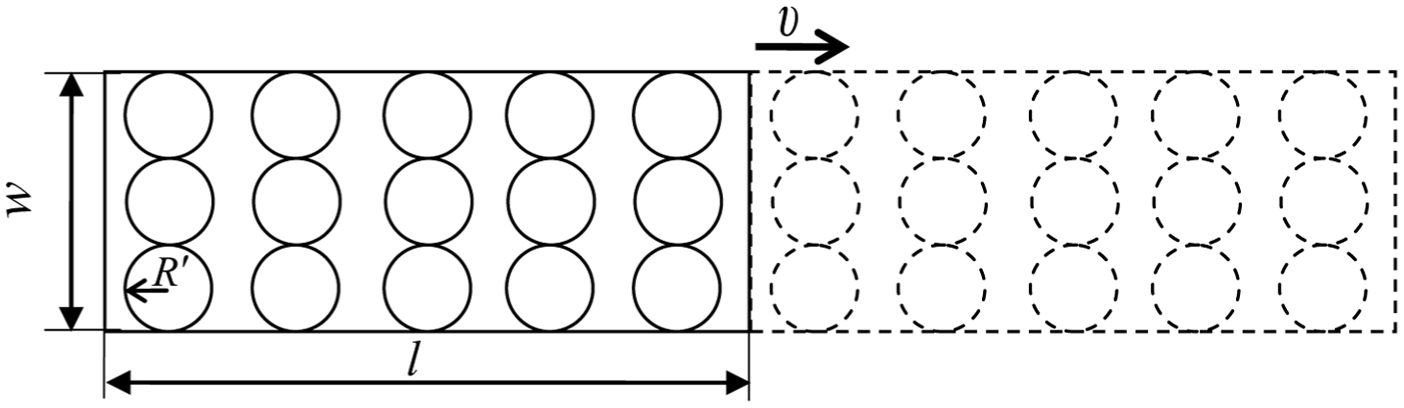
Smooth rigid surface with uniform asperities slides for the distance l (top view).

Figure 4 shows the arrangement of the asperities on the upper rigid surface of model III with the nominal area S (l × w). The asperities are packed closely in the first column from the left margin. The other asperities are equidistantly arranged in columns along the length direction. If n is the number of asperities on the upper surface, D is the surface density of asperities of the upper surface, R′ is the mean radius of the asperities, i is the number of asperities in one column, and j is the number of columns, then

n = SD = lwD

(5)

i \cdot 2 R' = w

(6)

ij = n

(7)

Substituting equations (5) and (6) into equation (7), the number of columns j will be expressed as

j = 2 R' lD

(8)

When the upper rigid surface slides on the lower surface for the distance l, as shown in the top view in Figure 4, each asperity column will also slide over the length of l. The trajectory of each asperity column will form a rigid plane that contacts with the lower surface, and the contact state is equivalent to that of model II in Figure 2. The number of the contacted asperities is m in model II, so the number of contacts between asperities during the stroke of one column is also m. Since there are totally j columns on the upper surface, the total number N₁ of contacts between asperities in the sliding distance l will be

N_{1} = mj

(9)

Substituting equations (3) and (8) into equation (9) gives

N_{1} = 2 R' lDn \int_{h}^{\infty} ψ (z) dz

(10)

Substituting equation (5) into equation (10) gives

N_{1} = 2 R' lS D^{2} \int_{h}^{\infty} ψ (z) dz

(11)

Equation (11) presents the number N₁ of dynamic contacts between asperities of the two flat rough surfaces when sliding for one cycle length l. For a given sliding stroke L, the number N of dynamic contacts between asperities through the sliding process will be

N = \frac{L}{l} N_{1}

(12)

After substituting equation (11) into equation (12), it turns out

N = 2 SLR' D^{2} \int_{h}^{\infty} ψ (z) dz

(13)

The distribution function of asperity height z, ψ(z) in equation (13), usually follows the normal distribution with the arithmetic mean of µ and standard deviation of σ′ (σ′ is expressed by equation (1)). It can be seen in Figure 5 that the height of asperities is more likely in the exponential distribution in the range of h ∼ +∞; h is the spacing distance between the two reference planes on the contact rough surfaces; therefore, ψ(z) in equation (13) can be expressed approximately by a exponential function as

ψ (z) = \frac{1}{σ'} e^{- z / σ'}

(14)

Figure 5.

Distribution curve of asperity height.

And the relative error of the approximation is not more than 9.3% in the range of h∼+∞. Then, the integration expressions in equation (13) can be calculated analytically as

\int_{h}^{\infty} ψ (z) d z = e^{- h / σ'}

(15)

Substituting equation (15) into equation (13) leads to

N = 2 SLR' D^{2} e^{- h / σ'}

(16)

Equation (16) presents the analytical expression of the number N of elastic dynamic contacts between asperities of two flat rough surfaces during sliding process. As shown in equation (16), the number of elastic contacts of asperities depends on the surface topography parameters R, D, and σ; nominal contact area S; sliding distance L; and spacing h between two rough surfaces. Since the elastic contact states of asperities are the same during the forward and backward movements of the sliding surface when it slides on the fixed surface, equation (16) is applicable to both one-way and reciprocating sliding process.

Simulation modeling of dynamic contact of asperities between nominal rough planes

Mathematical descriptions of nominal rough planes

Two rough surfaces and the 3D coordinate system are shown in Figure 6(a). For the upper surface, the length is l and the width is w. The contact area between the upper and lower surfaces is S = lw. The spacing between the surfaces is h. The sliding distance of the upper surface is L. As described as Figure 1, the asperities of rough surfaces in Figure 6(a) are composed of a series of spherical segments with the same radius and different heights. For the upper and lower surfaces, the radii of asperity are R₂ and R₁, respectively; the distribution density of asperity is D₂ and D₁, respectively; the standard deviation of the asperity height distribution is σ₂ and σ₁, respectively. As shown in the top view of asperities (Figure 6(b)), the asperities are the circles with different radii, and the asperity position can be determined by the coordinate values of its vertex in the x-axis and y-axis position of the rough surface. The size of each asperity can be determined by the apex height z. The greater the height z, the greater the radius of spherical segment c, as shown in Figure 6(c). Therefore, all the asperities of the upper and lower surfaces can be uniquely determined by their 3D coordinate values of the vertices. The asperities on the upper and lower surfaces are indicated by the arrays of (X, Y, Z) and (x, y, z), respectively. For the surface asperities are randomly distributed, the position coordinates (x and y) of asperities are the random variables in the length direction and the width direction. The height z is also a random variable with normal distribution. As shown in Figure 5, the normal distribution is determined by the topographical parameters, µ (the arithmetic mean of asperity height) and σ (the standard deviation of asperity height). The position coordinates and height coordinates of the asperities are generated with the random number generation function and the normal distribution function in MATLAB program.

Figure 6.

Mathematical descriptions of surface asperity: (a) the asperity model of rough surfaces in three-dimensional space coordinate system, (b) the top view of the surface asperities, and (c) the sectional view of single asperity.

Determination method of the dynamic contact of surface asperities during sliding process

When the sliding surface (the upper surface in Figure 6(a)) slides along the fixed surface (the lower surface in Figure 6(a)) for the length L, each asperity on the sliding surface also slides for the length L, and the sliding trajectory of each asperity forms the contact domain of the asperity, as shown in Figure 7. The asperity only contacts with the lower asperities which are located in the contact domain of the asperity. The range of the contact domain of the asperity is shown in Figure 8. When the position coordinates of the asperities on the lower surfaces meet equations (17) and (18), it means that the asperities are in the contact domain

X \leq x \leq X + L

(17)

Y - c \leq y \leq Y + c

(18)

where X and Y are the position coordinates of an asperity on the upper surface, c is the bottom radius of the asperity, and x and y are the position coordinates of an asperity on the lower surface. Let Z be the height of the asperity on the upper surface and z be the height of the asperity on the lower surface. h is the spacing between the two planes, as shown in Figure 6(a). If the upper asperity contacts with the lower asperity, it means that

Z + z > h

(19)

Figure 7.

Schematic diagram of the contact domain of an asperity on the sliding surface when it slides for the length L (top view).

Figure 8.

Range of the contact domain of an asperity on the sliding surfaces (X and Y are the position coordinates of the asperity).

In conclusion, only when the asperities on the lower surface satisfy equations (17)–(19), they are contacted with the asperities on the upper surface during sliding process.

Simulation process of the dynamic contact of surface asperities

The process of the simulation calculation was mainly composed of two loops, as shown in Figure 9. One loop is used to define the contact domain of the asperities on the upper sliding surface. Another loop is used to determine whether the asperities on the lower fixing surface are in the contact domain and whether they are contacted with the upper asperities. Ultimately, the dynamic contact between asperities during sliding process is cumulatively calculated to obtain the dynamic contact parameter, i.e. total number of contacts between asperities.

Figure 9.

Simulation calculation flowchart.

Simulation experiments

The topography of the machined rectangular sample was measured with Taylor Hobson surface topography instrument (Figure 10(a)) to obtain various statistical parameters of surface topography, including height parameter, functional parameters, spatial parameters, hybrid parameters, feature parameters, and so on. With the statistical parameters, automatic fitting with 3D microscopic surface topography is available, as shown in Figure 10(b). For the testing rectangular surface, the 3D topographical height parameters (the average height µ and the standard deviation σ) and feature parameters (the average radius of the asperities R and the distribution density of asperities D) are respectively 0.6107 µm, 0.7607 µm, 85.4 µm, and 111.6690 mm⁻².

Figure 10.

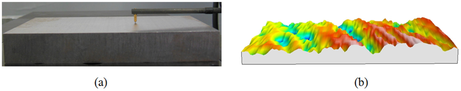
Topography measurement of a nominal rough plane: (a) testing surface and (b) 3D microscopic topography of the surface.

Based on these topography parameters, the following simulation experiments a–f with single variable were designed to analyze the influence of each factor (as shown in equation (16)) on the number of asperity contacts between two rough planes, wherein the topographical parameters (R, D, and σ) of the upper and lower surfaces are the same. Since the rough surface was randomly generated with the statistical topography parameters in the simulation model, even the same topography parameters will give different simulation results within a certain range for every calculation. Therefore, the simulation calculation was performed for 50 times with each set of parameters, and the average value was selected as the final simulation result, that is, the total number of contacts.

Case a, S is a variable. The invariants are L = 500 µm, h = 1.1 µm, R = 85.4 µm, D = 111.6690 mm⁻², and σ = 0.7607 µm. The values of variable S and the simulation results are shown in Table 1.

Table 1.

Simulation results of case a.

S (×10⁴ µm²)	Simulation results	Standard deviation
25	41	2.35
50	87	3.61
75	132	3.55
100	180	3.39
125	227	5.16

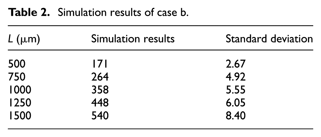
Case b, L is a variable. The invariants are S = 100 × 10⁴ µm², h = 1.1 µm, R = 85.4 µm, D = 111.6690 µm⁻², and σ = 0.7607 µm. The values of variable L and the simulation results are shown in Table 2.

Table 2.

Simulation results of case b.

L (µm)	Simulation results	Standard deviation
500	171	2.67
750	264	4.92
1000	358	5.55
1250	448	6.05
1500	540	8.40

Case c, h is a variable. The invariants are S = 100 × 10⁴ µm², L = 500 µm, R = 85.4 µm, D = 111.6690 µm⁻², and σ = 0.7607 µm. The values of variable h and the simulation results are shown in Table 3.

Table 3.

Simulation results of case c.

h (µm)	Simulation results	Standard deviation
0.3	220	5.21
0.6	211	3.85
0.9	193	4.62
1.1	177	4.41
1.4	140	3.69
1.7	101	2.62
2.0	73	1.82

Case d, R is a variable. The invariants are S = 100 × 10⁴ µm², L = 500 µm, h = 1.1 µm, D = 111.6690 µm⁻², and σ = 0.7607 µm. The values of variable R and the simulation results are shown in Table 4.

Table 4.

Simulation results of case d.

R (µm)	Simulation results	Standard deviation
45.4	81	3.07
85.4	171	5.01
125.4	260	4.59
165.4	348	6.84
205.4	437	8.09

Case e, D is a variable. The invariants are S = 100 × 10⁴ µm², L = 500 µm, h = 1.1 µm, R = 85.4 µm and σ = 0.7607 µm. The values of variable D and the simulation results are shown in Table 5.

Table 5.

Simulation results of case e.

D (µm⁻²)	Simulation results	Standard deviation
71.6690	65	2.84
91.6690	107	3.24
111.6690	161	4.40
131.6690	227	4.56
151.6690	301	5.73

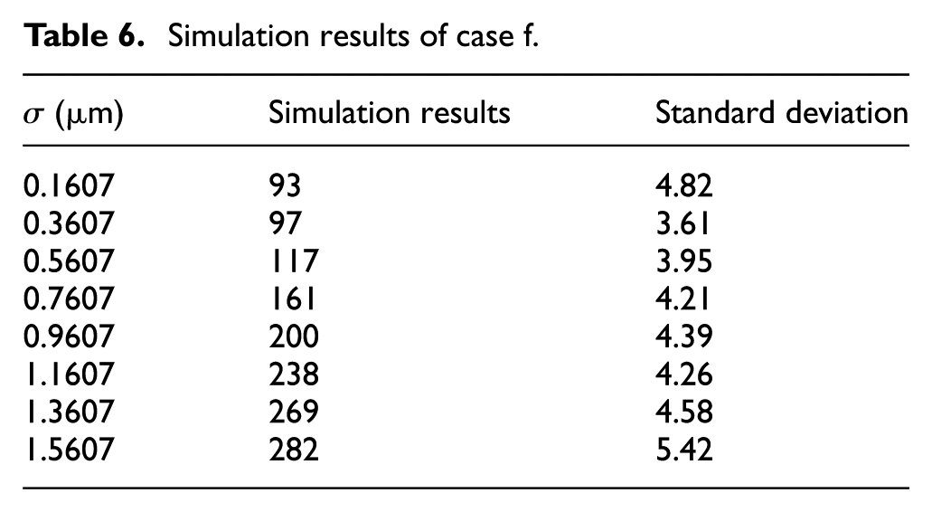
Case f, σ is a variable. The invariants are S = 100 × 10⁴ µm², L = 500 µm, h = 1.1 µm, R = 85.4 µm, and D = 111.6690 µm⁻². The values of variable σ and the simulation results are shown in Table 6.

Table 6.

Simulation results of case f.

σ (µm)	Simulation results	Standard deviation
0.1607	93	4.82
0.3607	97	3.61
0.5607	117	3.95
0.7607	161	4.21
0.9607	200	4.39
1.1607	238	4.26
1.3607	269	4.58
1.5607	282	5.42

Results and discussion

The theoretical values of number of asperity contacts for each simulation case in section “Simulation experiments” were calculated by analytical expression equation (16). With the comparison between the theoretical and simulation results, the rationality of the analytical model of asperity contacts can be validated.

Comparison between the theoretical values and the simulation values of case a

As shown in Figure 11, the curve of theoretical values is very close to that of simulation values with the relative deviation of 3.6%–14.6%, and they both indicate that N is in the linear increasing relationship with S. The consistent results indicate that equation (16) can reasonably reflect the relationship between N and S.

Figure 11.

Comparison between the theoretical values and the simulation values of the number of dynamic contacts under the conditions of different contact areas S.

Comparison between the theoretical values and the simulation values of case b

As shown in Figure 12, under different sliding distances, the theoretical values are very close to the simulation values, and the relative deviation is 6.3%–11.7%. The theoretical and simulation curves show that N is in the linear increasing relationship with L. The consistent results indicate that equation (16) can reasonably reflect the relationship between N and L.

Figure 12.

Comparison between the theoretical values and the simulation values of the number of dynamic contacts under the conditions of different sliding distances L.

Comparison between the theoretical values and the simulation values of case c

As shown in Figure 13, the theoretical curve and the simulation curve show some exponential relationship between N and h. When the spacing h increases more than a certain value (the value in Figure 13 is 1.1, which is approximately equal to the standard deviation σ′), the theoretical values are very close to the simulation values, and the minimum relative deviation is 2.9%. When the spacing is less than this value, the deviation between the theoretical values and the simulation values is increased with the decreased spacing, and the maximum relative deviation is 82.7%.

Figure 13.

Comparison between the theoretical values and the simulation values of the number of dynamic contacts under the conditions of different contact spacing h.

The large deviation is caused by the fact that the asperity height during the simulation calculation follows the normal distribution strictly. Contrastively, in the theoretical model, in order to obtain analytical expression equation (16), the exponential function equation (14) was used to express the distribution of asperity height during the integration. As shown in Figure 5, the normal distribution curve tends to be the exponential distribution when the spacing is larger than a certain value h; when the spacing is less than a certain value h, the normal distribution curve deviates from the exponential distribution. Thus, the deviation between the theoretical value and the simulation value is large in the small value range of h. Actually, when the two surfaces are in elastic contact, the spacing h between the two surfaces is approximately equal to the standard deviation σ′,¹⁵ and it cannot obtain those small values as shown in Figure 13. It is indicated that the theoretical model can be used to calculate the dynamic contacts of two rough planes under the elastic contact.

Comparison between the theoretical values and the simulation values of case d

As shown in Figure 14, under the condition of different asperity radii, the theoretical values of the number of asperity contacts are very close to the simulation values, and the relative deviation is 5.3%–24.7%. Equation (16) indicates that the number of asperity contacts N is in the linear increasing relationship with the composite radius R′. R′ can be calculated with Equation (2) and it is in the linear relationship with R. So N is in the linear increasing relationship with R in Equation (16). The simulation results shown in Figure 14 also indicate that N is in the linear increasing relationship with R. The consistent results indicate that equation (16) can reasonably reflect the relationship between N and R.

Figure 14.

Comparison between the theoretical values and the simulation values of the number of dynamic contacts under the conditions of different asperity radii R.

Comparison between the theoretical values and the simulation values of case e

As shown in Figure 15, under the conditions of different asperity distribution densities D, the theoretical values are close to the simulation values. When the asperity distribution density is small, the theoretical values are very close to the simulation values, and the minimum relative deviation is 17.2%. When the asperity distribution density is large, the deviation between the theoretical values and the simulation values is increased, and the maximum relative deviation is 20.0%. It may be interpreted as follows: when the density is large, the asperity number is also large in the given surface area, and it is prone to produce contact interference (one asperity contacts with multiple asperities at the same time, and this contact state is considered as one contact) during the simulation of dynamic contact. Thus, the accumulated contact number is reduced. On the contrary, in the theoretical model, it is assumed that the contact occurs between two asperities, and the contacts among several asperities at the same time are considered as multiple contacts. Thus, the theoretical value is large. The simulation value curve and the theoretical value curve show the same exponential relationship, indicating that equation (16) can reasonably reflect the relationship between N and D.

Figure 15.

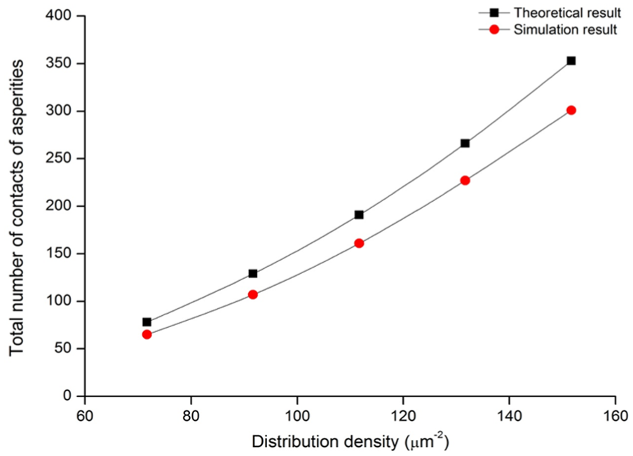
Comparison between the theoretical values and the simulation values of the number of dynamic contacts under the conditions of different distribution densities D.

Comparison between the theoretical values and the simulation values of case f

According to equation (16), the number of asperity contacts is in the exponential relationship with composite standard deviation σ′ of asperity height distribution. σ′ and σ show the linear relationship (see equation (1)). Thus, the theoretical values of N are also in the exponential relationship with σ, as shown in Figure 16. When σ is greater than a certain value (about 0.5), the theoretical value curve is very close to the simulation value curve, indicating that equation (16) can reasonably reflect the relationship between N and σ. When σ is <0.5, the theoretical values decrease rapidly, and the deviation between the theoretical value and the simulation value is large.

Figure 16.

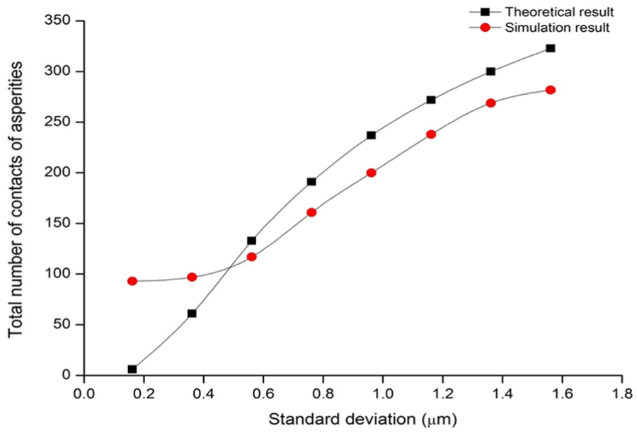
Comparison between the theoretical values and the simulation values of the number of dynamic contacts under the conditions of different standard deviations σ.

The deviation can be interpreted as follows: According to equation (13), during the theoretical calculation, the theoretical value is cumulatively integrated with the asperity height distribution function ψ(z) within the range (h ∼ +∞). As shown in Figure 17, with the decreasing σ, the normal distribution peak rapidly increases and the integration of ψ(z) within the range (h ∼ +∞) rapidly decreases. Thus, the theoretical values calculated using equation (13) rapidly decrease. For simulation calculation, as discussed in section “Mathematical descriptions of nominal rough planes,” the asperity height follows the normal distribution. As shown in Figure 17, when σ is decreased, the peak of the height distribution curve becomes high, indicating that the height of more asperities is concentrated to µ and the probability that 2Z > h (see equation (19), which is a condition of asperity contacts) becomes small. It means that the probability of asperity contact becomes small. Thus, in the small value range of σ, the simulation values also decrease with the theoretical values. But as can be seen in Figure 17, the difference in the concentration degree of asperity height distribution ψ(z) decreases with the decrease in σ, which means the influence of the change in ψ(z) on the simulation results is decreased with the decrease in σ. Thus, the simulation results obtained under the low σ will not show large variation as the theoretical results.

Figure 17.

Normal distribution curve under the conditions of different standard deviations σ.

For the commonly machined rough surfaces, the standard deviation σ of the height distribution of asperities is not small. According to the measurement results of the metal surface machined with precise grinder, the asperity height is 0.4314 µm, and the standard deviation is 0.5106 µm. The surface machined with other conventional machining methods shows the higher standard deviation. Moreover, the spacing h is decreased with the standard deviation σ of asperity height when the two surfaces are in elastic contact. According to Figure 17, when σ and h are decreased simultaneously, the integration of ψ(z) in the range (h ∼ +∞) in equation (13) will not change greatly. Therefore, the theoretical results will not show the large deviation as presented in Figure 16 for actual rough surfaces with elastic contact.

Conclusion

Based on the statistical contact theory, a dynamic contact model of rough planes under elastic contact state was established to calculate the total number of asperity contacts for engineering rough planes during sliding process.

A computer simulation model of the sliding contact between the rough planes was established to rapidly calculate the number of dynamic contacts during the sliding process.

Through the comparison between the theoretical values and simulation values of the dynamic contacts under different parameter conditions, it was verified that the modeling of the dynamic contact of asperities was reasonable, and the theoretical model correctly described the mathematical relationship between the number of asperity contacts and the major influencing factors. The dynamic contact model can provide a reference for the analysis of dynamic contact performance and microscopic fatigue damage of mechanical surfaces.

Footnotes

Academic Editor: Pranab Samanta

Declaration of conflicting interests

The author(s) declared no potential conflicts of interest with respect to the research, authorship, and/or publication of this article.

Funding

The author(s) disclosed receipt of the following financial support for the research, authorship, and/or publication of this article: This work received the financial support from the National Natural Science Foundation of China under grant no. 51275083 and the Fundamental Research Funds for the Central Universities under grant N152303011.

References

Greenwood

Williamson

JBP

. Contact of nominally flat surface. P Roy Soc A: Math Phy 1966; 295: 300–319.

Etsion

. Elastic-plastic contact analysis of a sphere and a rigid flat. J Appl Mech: T ASME, 2002; 69: 657–662.

Kogut

Etsion

. A finite element based elastic-plastic model for the contact of rough surfaces. Tribol T 2003; 46: 383–390.

Webster

Sayles

. A numerical model for the elastic frictionless contact of real rough surfaces. J Tribol: T ASME 1986; 108: 314–320.

Furey

. Metallic contact and friction between sliding surfaces. ASLE Trans 1961; 4: 1–11.

Yaqoob

Winogrodzka

Fischer

. Pre-sliding behaviour of single asperity contact. Tribol Lett 2013; 49: 553–562.

Mulvihill

Kartal

Nowell

. An elastic–plastic asperity interaction model for sliding friction. Tribol Int 2011; 44: 1679–1694.

Karupannasamy

de Rooij

Schipper

. Multi-scale friction modelling for rough contacts under sliding conditions. Wear 2013; 308: 222–231.

Raeymaekers

Etsion

. Dynamic elastic contact model for sliding realistic rough surfaces. In: Proceedings of the STLE/ASME 2010 international joint tribology conference, San Francisco, CA, 17–20 October 2010. New York: ASME.

10.

Soom

Chopra

. In search of dynamic effects in dry sliding friction. Tribology S 2001; 39: 55–59.

11.

Chang

. The effect of surface roughness and contaminant on the dynamic friction of porcelain tile. Appl Ergon 2001; 32: 173–184.

12.

Whitehouse

Archard

. The properties of random surface of significance in their contact. P Roy Soc A: Math Phy 1970; 316: 97–121.

13.

Onions

Archard

. The contact of surfaces having a random structure. J Phys D Appl Phys 1973; 6: 289–304.

14.

Bush

Gibson

Keogh

. Strongly anisotropic rough surfaces. J Lubric Tech: T ASME 1979; 101: 15–20.

15.

Gibson

. The surface as a random process. In: Thomas

(ed.) Rough surfaces. London: Longman, 1982, pp.87–110.

16.

McCool

. Predicting microfracture in ceramics via a microcontact model. J Tribol: T ASME 1986; 108: 380–386.

17.

Kotwal

Bhushan

. Contact analysis of non-Gaussian surfaces for minimum static and kinetic friction and wear. Tribol T 1996; 39: 890–898.

18.

Majumdar

Bhushan

. Fractal model of elastic-plastic contact between rough surfaces. J Tribol: T ASME 1991; 113: 1–11.

19.

Bhushan

Majumdar

. Elastic-plastic contact model of bifractal surfaces. Wear 1992; 153: 53–64.

20.

Almqvist

Campaná

Prodanov

. Interfacial separation between elastic solids with randomly rough surfaces: comparison between theory and numerical techniques. J Mech Phys Solids 2011; 59: 2355–2369.

21.

Ortiz

Siedlecki

Remon

. Optical coherence tomography for quantitative surface topography. Appl Optics 2009; 48: 6708–6715.

22.

Postawa

Rzeznik

Paruch

. Depth profiling by cluster projectiles as seen by computer simulations. Surf Interface Anal 2011; 43: 12–15.

23.

Wen

Huang

. Principles of tribology. 3rd ed.Beijing, China: Tsinghua University Press, 2008.

24.

Greenwood

Tripp

. The contact of two nominally flat rough surfaces. Proc Instn Mech Engrs 1971; 185: 625–633.