
Abstract
In urban rail transport, train timetable plays a crucial role, whose quality determines the whole system’s performance to a large extent. In practical urban rail operation, two contradictive aspects—service quality and operation cost—should be considered during train scheduling. A good train timetable should achieve considerable service quality with as little operation cost as possible. Previously, many studies have been conducted specific to urban rail train scheduling, although most of them do not put enough emphasis on its multi-objective nature. In this article, therefore, Pareto optimal urban rail train scheduling which can give more instruction to practical operation is studied. First, referring to some existing studies, the problem is reasonably defined, which takes time-dependent origin–destination demand as the input and aims at minimizing the passengers’ total travel time and the number of used train stocks. Then, an efficient iteration algorithm and a valid train stock assignment procedure are designed to calculate the passengers’ total travel time and required train stock number, respectively. On that basis, the studied problem is reasonably formulated as a bi-objective optimization model and a Pareto-based particle swarm optimization procedure is designed to solve it. Finally, with two different scaled urban rail lines, the whole methodology is illustrated and the algorithm is tested.
Keywords
Introduction
Public transport has been recognized as one of the most effective methods to reduce urban traffic congestion. Among the common public transport modes, rail transport is more favored due to its high speed and capacity. Nowadays, in almost all metropolises around the world, rail transit is applied and plays an important role in the daily trips of residents.
Compared with other transport modes, the operation of rail transport is more dependent on advance planning, which generally consists of five phases: 1 demand analysis, line planning, train timetabling, rolling stock planning, and crew scheduling. In this planning system, train timetable plays a crucial role, which provides the foundation for the following phases, that is, rolling stock and crew scheduling. The quality of train timetable, therefore, determines the performance of the whole system to a large extent. In early times, when train timetabling can only be conducted manually, the quality of timetable was mainly determined by designer’s experience. With the development of computer technology, automatic train timetabling draws more and more attention and many studies have been conducted on it. Some studies are focused on the description of designer’s experience with computer language,2,3 while more other studies are conducted from the perspective of mathematical optimization.4–11
As a particular form of rail transport, the operation of urban rail transit also requires well-predefined train timetable. Compared with intercity railways, however, urban rail systems generally have the following features: 12
Detailed origin–destination (OD) demand information can be easily collected through the automatic fare collection (AFC) system.
Urban rail line is always designed as double-track and each direction has a separate rail track. Hence, trains in different directions do not interact and can be scheduled separately.
Skip-stop pattern is not allowed and trains make stop at every station they pass.
Trains get similar performance (speed), so trains do not overtake each other during operation.
With these features, the train timetabling problem of urban rail transport is remarkably different with that of intercity rail system. On one hand, due to the absence of train crossing and overtaking, the decision variables in timetabling are much reduced. At the meantime, with the systematic travel demand information, the timetabling can be conducted in a more refined and demand-oriented manner.
Previously, quite a number of studies have been conducted specific to urban rail train timetabling problem and most of them are from mathematical optimization perspective. Cury et al. 13 proposed a nonlinear optimization model for the train timetabling problem of São Paulo Underground Railway System. In that model, a specific number of trains are given and the headways between consecutive trains need to be determined to minimize the total cost which combines the passengers’ total waiting time, the number of trains, the deviation between the actual number and the desired number of the passengers in the train, and the deviation between the actual and reference control sequence. Also on the train timetabling problem of São Paulo Underground Railway System, Wânderson and Basílio 14 proposed a new linear programming approach, which can be solved more efficiently. This approach, however, is only suited for periods of time where the passenger demand can be considered constant. Kwan and Chang 15 studied the scheduling of rapid transit systems from Pareto optimization perspective, in which operating costs and passenger dissatisfaction level are considered as optimization objectives and average train frequency, average dwell time, average coast level, and average layover time are taken as variables, and proposed a heuristic-based evolutionary algorithm to achieve that. Niu and Zhou 16 studied the urban rail timetabling under oversaturated conditions, taking into consideration that the passengers may not be able to board the next arrival train due to the limited train capacity. With a reasonable description of passenger loading and departure events, they proposed a nonlinear train scheduling model, whose objective is to minimize the total number of waiting passengers and weighted remaining passengers. Zhu et al. 17 also studied the urban rail timetabling with capacity constraints. In their study, the capacity constraint of station is also considered and a simple simulation model is proposed to calculate the passenger waiting cost. On this basis, a single-objective optimization model is proposed and generic algorithm is applied to solve it. Wang et al. 12 studied the train scheduling problem for an urban rail transit network. With an event-driven model describing network status, a nonlinear non-convex optimization model is designed, in which the objective function is a weighted sum of the passengers’ total travel time (PTTT) and trains’ energy consumption.
As can be seen, the multi-objective nature of urban rail timetabling has been widely recognized and the objectives used in the existing studies can be divided into two main aspects—service quality and operation cost. However, the existing studies do not cope with the multiple objectives very well. In most of the above studies, simple weighted aggregation is used to integrate the multiple objectives.12–14,16,17 However, the practicability of these weighted aggregation methods cannot be guaranteed, since there is still no definite unified opinion on how to determine the weight proportion of each aspect. In contrast, Pareto optimality method is more practical, which can provide more information to operators when determining an optimal train timetable, that is, list more compromise solutions to let the operator choose according to the circumstances of urban rail system. Kwan and Chang 15 introduced Pareto optimality, but the variables in their model are relatively simplified, which limits its application. In this article, therefore, a Pareto optimal urban rail train scheduling problem, which is more realistic and helpful, is proposed, in which the PTTT and the number of used train stocks are chosen as objectives to represent the service quality and operation cost, respectively.
The rest of this article is organized as follows. In the next section, the studied problem is elaborated and the notations used in this article are defined. Then, in section “Performance assessment of urban rail train timetable,” an efficient iteration algorithm and a valid train stock assignment procedure are designed to calculate the PTTT and the required train stock number, respectively, based on which a bi-objective mathematical optimization model is proposed in section “Model formulation.” In section “Pareto optimal solution using generalized PSO,” a Pareto-based particle swarm optimization (PSO) procedure is designed to solve the proposed model. After that, in section “Numerical example,” two example urban rail lines are introduced to illustrate the proposed methodology and test the algorithm. Finally, conclusions and discussions are given in section “Conclusion and discussions.”
Problem statement
With reference to the existing studies,13,14,16,17 a bi-directional urban rail line with only one rail yard located at one end is considered in our studies, whose layout is shown in Figure 1. The station on the end where the yard is located is called the start terminal, while the station on the other end is called return terminal. The direction from the start terminal to the return terminal is defined as down-bound and the opposite direction is up-bound. The stations are numbered as 1, 2,…, m sequentially along the down-bound direction. Among all the stations, only the two terminal stations are equipped with crossovers and can accommodate train turning-back.

Layout of the studied urban rail line.
During operation, the trains depart from the yard and enter the line from the start terminal. After a down-bound trip with making stop at each station, trains reach the return terminal, in which they are emptied and then conduct turning-back to begin an all-stop up-bound trip. When the trains return to the start terminal, they are faced with two choices—going back into the rail yard or turning back to start a new round. In this process, as analyzed in section “Introduction,” the trains have the similar performance so that they do not overtake each other and trains are assumed to follow the same running time in each section and the same dwell time at each station.16,17 Besides, the headway between the arrivals of two consecutive trains at the start terminal from the rail yard should ensure that no conflict happens between them in the following operation procedures. More specifically, the headway between the arrivals of two consecutive trains at the start terminal must be not less than the minimum safety headway between two consecutive running trains in the section, two consecutive arrivals at each station, or two turning-backs in the return terminal.
As for the passengers, their arrivals at each station follow a non-homogeneous Poisson process with arrival rate varying with time. In order to describe that, the scheduled time horizon is typically divided into several time periods and the arrival rate or the number of arrivals at each station in each time period is given. On the platform, the passengers board the train on a first-come-first-served (FCFS) basis, which has been proven a valid assumption in urban transit-related study.
On the above conditions, the train timetable can be considered to be composed of a series of train round trips (abbreviated as TRTs), each of which is made up of a down-bound trip and an up-bound trip. Once the start time of each TRT is determined, a definite train timetable can be derived. Therefore, the decision variables of the train timetabling problem here are the start times of these TRTs. As for the objective, PTTT and the required number of train stocks, which represent transit service quality and operation cost, respectively, are chosen as the main performance criteria of train timetable, as analyzed in section “Introduction.” To summarize, the train timetabling problem studied here can be described as determining the start time of each TRT to achieve a minimum PTTT with as few train stocks as possible.
Based on the above statements, the parameters and variables used in this study are identified. The corresponding notations are listed in Appendix 1.
Performance assessment of urban rail train timetable
Calculating PTTT
As elaborated in section “Introduction,” the key point in calculating PTTT is the reasonable consideration of train capacity constraint. Here, in order to achieve efficient calculation of PTTT under capacity constraints, an iteration algorithm is proposed.
As analyzed in section “Problem statement,” once the decision variables
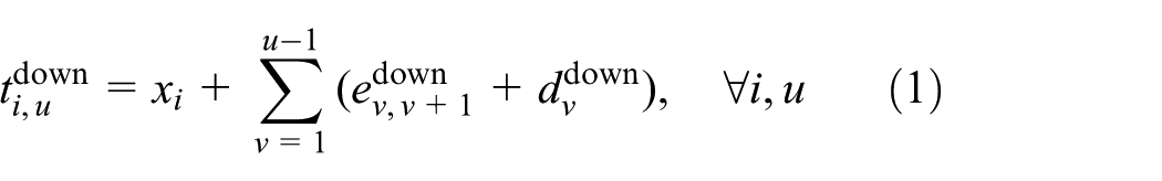
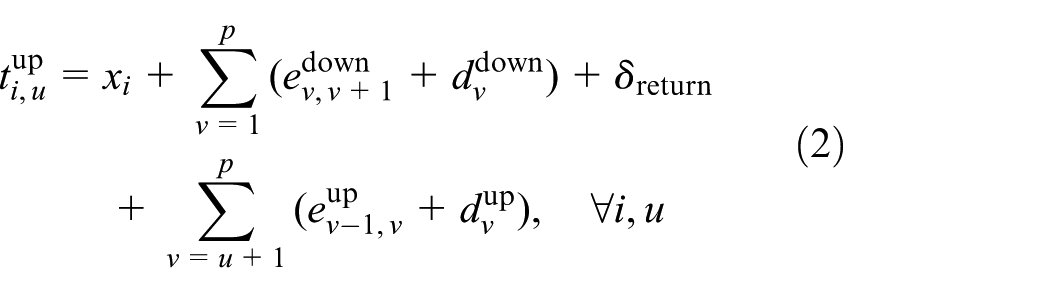
Since the trains need to be emptied before turning back at the return terminal, the up-bound and down-bound passenger transit processes are relatively separated. Therefore, given a definite train timetable, the PTTT of each direction can be calculated separately. In the following, the calculation of down-bound PTTT (i.e.
Step 0: initialization. Set
Step 1: calculate the composition of down-bound passengers who are trying to get on the train of round trip i from the platform of station
1. If the TRT i is the first one in the timetable, that is,

2. If the TRT i is not the first one, that is,

Step 2: when the train of round trip i arrives at station
Update
Step 3: update
Step 3.1: set
Step 3.2: if
Step 3.3: if


If

where
Step 3.4: if
Step 4: if
Step 5: if
The above procedure is further illustrated in Figure 2. Through this procedure, the expected total travel time of down-bound passengers can be efficiently calculated. In a similar way, the up-bound PTTT


Calculation of down-bound PTTT.
Determining number of train stocks required
In practice, rolling stock assignment needs to be conducted after train timetabling so that the timetable can be actually implemented. Here, a valid rolling stock assignment procedure is proposed to determine the number of train stocks required for a specific train timetable.
First, an n-dimensional square matrix


Given a specific train timetable, the start times of all the TRTs
Step 0: set
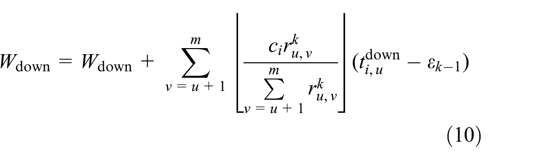
Step 1: determine which round trips’ train stock can undertake a new round trip through turning back at the start terminal. Step 1.0: set Step 1.1: check whether the train stock of round trip i can conduct turning-back at the start terminal. Step 1.1.0: set Step 1.1.1: if Step 1.1.2: check whether the train stock of round trip Step 1.1.3: if Step 1.1.4: if Step 1.2: determine which subsequent round trip this train stock undertakes after turning back at the start terminal. Check whether there is TRT starting from the start terminal after the time Step 1.3: if
Step 2: determine which round trips can be undertaken by the train stock returning to the rail yard from certain previous round trip. Step 2.0: set Step 2.1: if Step 2.2: if there is TRT j returning to start terminal before the time Step 2.3: if
Step 3: extract the columns whose elements are all 0 from the matrix
Model formulation
On the basis of the theories proposed in section “Performance assessment of urban rail train timetable,” the multi-objective optimization problem proposed in section “Problem statement” can be formulated. In this section, the objective functions and constraints of the mathematical model are designed.
Objective function
Given a specific train timetable, the corresponding PTTT can be calculated using the iteration algorithm proposed in section “Calculating PTTT” and the number of train stocks required can be determined through the rolling stock assignment procedure proposed in section “Determining number of train stocks required.” Here, in order to facilitate description, these two procedures are abstracted as two functions


where

Constraints
Three kinds of constraints are considered in this model, which are formulated, respectively, in the following.
Operation time constraints
In practice, the operation time of urban rail line is always clearly defined and all the transit services should be conducted within the specified time horizon. In this study, therefore, the start times of TRTs are all limited predefined time horizon, that is

where
Safety headway constraints
As analyzed in section “Problem statement,” the start times of TRTs should ensure no conflict happens in the following train operations. Therefore, the headway between the start times of two consecutive round trips should be larger than the minimum safety headway between the two consecutive running trains in the section, two consecutive arrivals at each station, and two consecutive turning-backs at the return terminal. Synthesizing these safety requirements, a minimum safety headway

Unmet demand constraint
When calculating the PTTT using the iteration algorithm proposed in section “Calculating PTTT,” the unmet travel demands

Generally, unmet travel demand has an adverse effect on the transit service quality of urban rail transit, which should be avoided as much as possible. Therefore, in order to guarantee the service quality, the amount of unmet demands should be limited in a reasonable range, that is
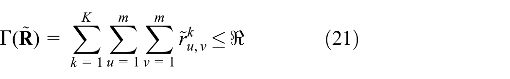
where
Pareto optimal solution using generalized PSO
As can be seen, the problem we study here is a quite complex combinatorial optimization problem, which is usually solved by heuristic algorithms.15–19 Besides, as analyzed in section “Introduction,” many existing studies formulate the urban rail train scheduling as multi-objective optimization and most of them choose weighted aggregation method to handle the multiple objectives.14,15,17 In this study, Pareto optimization, which is considered more reasonable in handling contradictive objectives, is introduced to solve the proposed multi-objective train scheduling problem and a generalized PSO procedure is applied to achieve this solution.
Model adjustment and Pareto solution
In order to facilitate the PSO operation, the model proposed in section “Model formulation” is adjusted. The unmet demand constraint is introduced into the first objective with a large number M as penalty coefficient, that is

Then the whole model can be described as


where
According to the general theory of Pareto optimality, for two arbitrary solutions

it can be said that the solution
Pareto-based PSO
PSO is a widely used population-based stochastic search algorithm, which is proposed by Kennedy and Eberhart. 20 In PSO, each particle is endowed with three attributes—position, fitness, and velocity. Generally, the position of a particle corresponds to a particular solution in the solution space and the fitness corresponds to the objective function value of this solution. During iteration, the position of each particle is updated constantly, through which the solution space is searched. In classic PSO, the updates of particles’ positions are typically controlled by their velocities, that is

where I is the iteration index and p is the particle index.
In addition, the velocities of the particles are also iteration-varying. On each iteration, the velocity of each particle needs to be adjusted according to some visited positions that achieve a good fitness, that is

where
Compared with other evolutionary algorithms, PSO achieves considerable computational accuracy with a much simplifier procedure and faster convergence rate. 21 Since being proposed, PSO has been widely used in various research areas, especially in traffic and transportation.22–26 In this process, the classic PSO has often been extended to accommodate different situations. One successful example of these extensions is the multi-objective PSO, that is, MOPSO. 27 In the past decade, a number of studies have been conducted on MOPSO and many useful theories have been proposed. Based on these existing theories, a Pareto MOPSO is designed to solve the proposed multi-objective train timetabling problem.
Main algorithm
Compared with single-objective PSO, MOPSO has some significant differences, one of which is the determination of
Step 0: set
Step 1: calculate the objective vectors of each particle. On this basis, update the external archive.
Step 2: update
Step 3: if
Step 4: set
The key points in above procedure include the following:
Initializing the particle swarm;
Updating the external archive;
Determining each particle’s personal best position and the global best position;
Updating velocity and position of each particle.
In the following parts, with the existing related theories, these key points are reasonably designed according to the features of the studied problem.
Swarm initialization
As can be seen, the main work during initial swarm generation is to set initial position and velocity for each particle, which influences efficiency of the whole algorithm to a large extent. Here, to solve the proposed model, the initial position and the velocity of the particles are generated in the following way.
Initial position
For each particle, the initial position is obtained through the following procedure:
Step 0: set
Step 1: set
Step 2: if

where rand[] is a function which returns a random integer within the specific interval, and go back to Step 1. Otherwise, stop.
Initial velocity
In order to guarantee the feasibility of particles’ position after first iteration, the initial velocity of each particle is generated as follows:
Step 0: set
Step 1: set
Step 2: if

and go back to Step 1. Otherwise, stop.
Archive maintenance
In order to reduce the computation cost, the size of external archive is typically limited. When a new non-dominated solution is obtained, the archive is updated through the following procedure:
Step 1: check whether these solutions in the archive are dominated by the new obtained solution. If yes, remove them and insert this new solution into the archive. If no, continue.
Step 2: check whether the size of archive reaches the ceiling. If no, then directly insert this new solution into the archive. If yes, continue.
Step 3: compare the performances of solutions in the archive and the new solution. If the worst solution in the archive is still better than the new one, then drop the new solution. Otherwise, replace the worst solution with the new obtained one.
To achieve this procedure, a definite approach for assessing the performance of non-dominated solution must be given. In our study, considering the penalty item in the first objective, a modified density-based approach is proposed. Given a set of non-dominated solutions of the studied problem
Step 1: select the solutions that do not satisfy constraint (21), set their fitness as
Step 2: for the remaining solutions, normalize their coordinates in the objective space according to

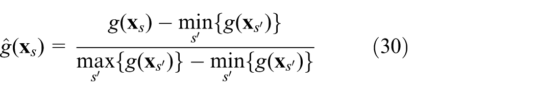
where
Step 3: for each remaining solution
Determining personal and global best position
On each iteration, the personal best position of each particle is determined simply according to Pareto dominance, that is, if the new position
As for global best position, the fitness calculation procedure proposed in the last section needs to be conducted on the archive again, and the non-dominated solution with maximum fitness is chosen to be the new
Updating position and velocity
On each iteration, the position and velocity of each particle are updated according to equations (25) and (26). Here, the control parameters in equation (26) are set as follows:
1. The inertia weight coefficient
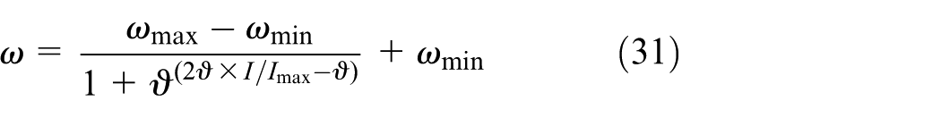
where
2. The acceleration constants

Then the evolutionary factor is calculated as

where

Furthermore, in order to guarantee the feasibility of particles’ positions in next iteration, the velocity of each particle needs to be examined and revised if not feasible. Relative procedure is as follows:
Step 0: set
Step 1: check whether
Step 2: set
Numerical example
Small-scaled example
First, the proposed methodology is tested on a fictitious small-scaled urban rail line, whose layout is shown in Figure 3. As can be seen, the line contains four stations. The numbers labeled between two adjacent stations specify the running time of train in this section along the corresponding direction, and the numbers labeled at the start and return terminal represent the required times for turning-back at these two stations. For this example line, a 4-hour OD travel demand data are collected, which are not listed here due to the limited space. Besides, on this specific line, the train dwell time at each station is 2 min, the minimum safety headway between the start times of two consecutive TRTs, that is,

Layout of the small-scaled example urban rail line.
Under a MATLAB 9.0 environment, the proposed methodology is implemented to conduct Pareto optimal train scheduling for this specific line. Based on that, the designed algorithm is tested.
First, different control parameter settings are compared. For the inertia weight coefficient

Comparison between different settings of inertia weight coefficient: (a) Variation of the number of infeasible solutions and (b) Variation of the number of non-dominated solutions.
For the acceleration constants

Comparison between different settings of acceleration constants: (a) Variation of the number of infeasible solutions and (b) Variation of the number of non-dominated solutions.
Moreover, based on the optimization toolbox provided by MATLAB, this example is further calculated by a branch and bound (BAB) procedure, and the result is compared with that of the proposed algorithm, as shown in Figure 6. As can be seen, the Pareto front obtained by PSO is almost as good as the result obtained by BAB. However, the PSO is much more efficient than BAB. When solving this small urban rail scheduling problem, PSO spends about 14 min while BAB spends more than 55 min. Therefore, the designed PSO procedure can achieve an adequate train scheduling with more reasonable time consumption.

Comparison between PSO and BAB.
Practical-sized example
Setup
Using the proposed methodology, train scheduling for a practical-sized urban rail line is conducted. This line contains 10 stations. Its layout, section running times, and turning-back times are shown in Figure 7, and the corresponding train dwell times are listed in Table 1. For this rail line, the OD demand statistics are collected for every 30 min of a whole day. Due to the limited space, only the distribution of passenger arrivals and the total cross-sectional passenger flow volume in each section are presented here, as shown in Figures 8 and 9. Besides, the minimum safety headway between the start times of two consecutive TRTs, that is,

Layout of the practical-sized example urban rail line.
Train dwell time at each station on the second example line.


Distribution of passenger arrivals on the second example line.

Total cross-sectional passenger flow volume in each section on the second example line.
Pareto optimal train scheduling
With the TRT number defined as 90, train timetabling for the example rail line is conducted using the designed MOPSO. The related parameters are set as shown in Table 2. After 100 iterations, a reasonable Pareto front is obtained as shown in Figure 10.
Parameter setting.


Pareto front.
As can been seen, as the number of train stocks is small (
Pareto optimal train timetable.

TRT: train round trip.
Conclusion and discussions
In this article, a Pareto optimal urban rail train scheduling problem is studied. Based on a representative layout of urban rail line, the studied problem is well defined as bi-objective optimization. Two innovative theories are proposed: an effective iteration algorithm to calculate PTTT and a valid train stock assignment procedure to obtain the number of used train stocks. Based on these theories, the problem is reasonably formulated. Then, based on general framework of MOPSO, a specific MOPSO is designed for the studied problem. Through the numerical experiment on two different scaled examples, the effectiveness of the designed algorithm is illustrated.
As for further research, several extensions can be considered. First of all, to further improve the practicability of obtained timetable, the dwell times of trains at stations should be determined according to the corresponding alighting and boarding process instead of predefined. Second, in the initial swarm generation of PSO, the unmet demand constraint can be further taken into account, so that the procedure can be simplified and the convergence rate of the whole algorithm can be improved. Third, the methodology should be tested under real context to verify its effectiveness in solving practical urban rail train scheduling problem.
Footnotes
Appendix 1
Acknowledgements
The authors are grateful to the editor and reviewers for their valuable suggestions which improved the article.
Academic Editor: Gang Chen
Declaration of conflicting interests
The author(s) declared no potential conflicts of interest with respect to the research, authorship, and/or publication of this article.
Funding
The author(s) disclosed receipt of the following financial support for the research, authorship, and/or publication of this article: This work was supported by the National High Technology Research and Development Program of China (2015AA016404), the Scientific Research Development Plan of China Railway Company (2014X010-B), and the Fundamental Research Funds for Central Universities of China (2015B11714).