Sage Journals: Discover world-class research

Abstract

A Y-type urban rail transit is composed of a trunk and a branch, and the passenger demand has the characteristics of multidirectional and unbalanced. It is important to design routing planning of Y-type urban rail transit and provide reasonable service for passengers with acceptable operational cost. In this study, a routing planning design model was proposed for Y-type urban rail transit aimed at minimizing the passenger travel time and train operating distance. The decision variables of the model were the locations of turn-backs and the departure frequencies of the train routings in the multi-routing planning. The constraints of passenger demand and line condition were considered. The multi-objective model was turned into a single-objective model by giving weight values to the objectives. Then a genetic algorithm was applied to obtain optimal solutions of the proposed model. Finally, a case study was conducted, and the optimal solutions under different forms of multi-routing planning with different weight values were analyzed. The results showed that when the weight of the passenger travel time increased to a certain level, the optimal solution changed from a two-routing planning to a three-routing planning, and the latter one could better meet the characteristics of the passenger.

Keywords

Urban rail transit Y-type line routing planning multi-routing passenger demand

Introduction

Y-type lines are those lines starting as heavily traveled trunk lines from the city center outward and then dividing into a greater number of lines with lower loads serving large, often low-density areas.¹ Y-type lines can attract more passengers to increase profit by expanding service areas, so the adoption of multi-routing mode may make the train routing planning better satisfy the multidirectional and unbalanced characteristics of passenger demand. There are many Y-type urban rail transit lines in operation such as Paris Line RER-A, Munich Metro Line 3 and Line 6, Guangzhou Metro Line 3, Beijing Subway Line Yanfang, and Hangzhou Metro Line 1.

Designing train planning of Y-type urban rail transit is to determine the locations of turn-backs and frequencies of the train routings subject to passenger demand and line condition. There exists much research on multi-routing planning in the field of urban public transport and railway; Furth² and Furth and Day³ propose methods on designing routing planning subject to a certain scale of vehicles and a balanced load factor, and propose the conception “schedule mode” which is the rate of the routings’ departure frequencies to cope with cyclical diagram; Ceder and colleagues^4–6 propose a multi-routing planning model aimed at minimizing the number of vehicles and the number of short-turn trips, and a strategy which combines short-turning, holding, and stop-skipping to reduce the passenger travel time and passenger transfers; Vijayaraghavan and Anantharamaiah⁷ propose to insert deadhead trips to meet passenger demand and reduce the number of vehicles; Tirachini and colleagues^8,9 and Site and Filippi¹⁰ propose a strategy combining short-turn and expressing to analyze the effects of departure frequencies, vehicle sizes, and turn-back stations on passengers and operator when the arrival of buses follows uniform distribution, and also Site and Filippi¹⁰ study the situation when the arrival of buses follows Poisson’s distribution; Canca et al.¹¹ propose a short-turn strategy to solve disruptions caused by heavy demand, aimed at diminishing passenger waiting time while preserving the quality of service; Jannson¹² optimizes the departure frequency and vehicle size to reduce passenger travel cost and operator cost; Chen et al.¹³ design an algorithm which can adjust train operation based on ordinary optimization and took a heavy haul railway as an example to prove that the solution can well satisfy the passenger demand.

However, the studies mentioned mainly focus on single lines, whose passengers do not need to transfer because all demands can be covered by the full-length routing which covers all the stations. However, the passenger demand of a Y-type line cannot be satisfied by a full-length routing, especially when the line connects the city center with the suburbs, so there exist some passengers who need to transfer. Also, the departure frequencies of the routings on the trunk line and the branch line are subject to the tracking interval because of the routings’ joint operation, which means different kinds of services operate on the same line. Therefore, the existing studies on single lines are not suitable for a Y-type line. The routing planning of Y-type line has been studied by a limited number of authors, and the studies mainly focus on designing the trunk line and branch line,¹⁴ proposing the variants of routing planning by qualitative description¹⁵ and optimizing the vehicle circulation under a certain routing planning.¹⁶

In summary, the studies on multi-routing planning did not consider the characteristics of Y-type line, and the studies on Y-type lines did not consider the influence of the departure frequencies and the turn-back stations. Thus, this article proposed a multi-routing planning model aimed at minimizing the passenger travel time and operator cost. Then the optimal solutions under different weights of passenger travel cost were obtained, and the influence of different types of routing planning on the passengers and the operator was discussed.

Description of the problem

Y-type line is usually composed of a trunk line and a branch line connected by a node station shown in Figure 1, in which O is the node station, AOB is the trunk line (named Trunk), and OC is the branch line (named Branch). Usually, the passenger flow of the trunk is larger than that of the branch.

Figure 1.

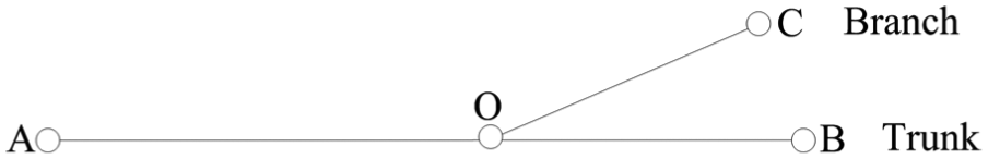
Components of Y-type line.

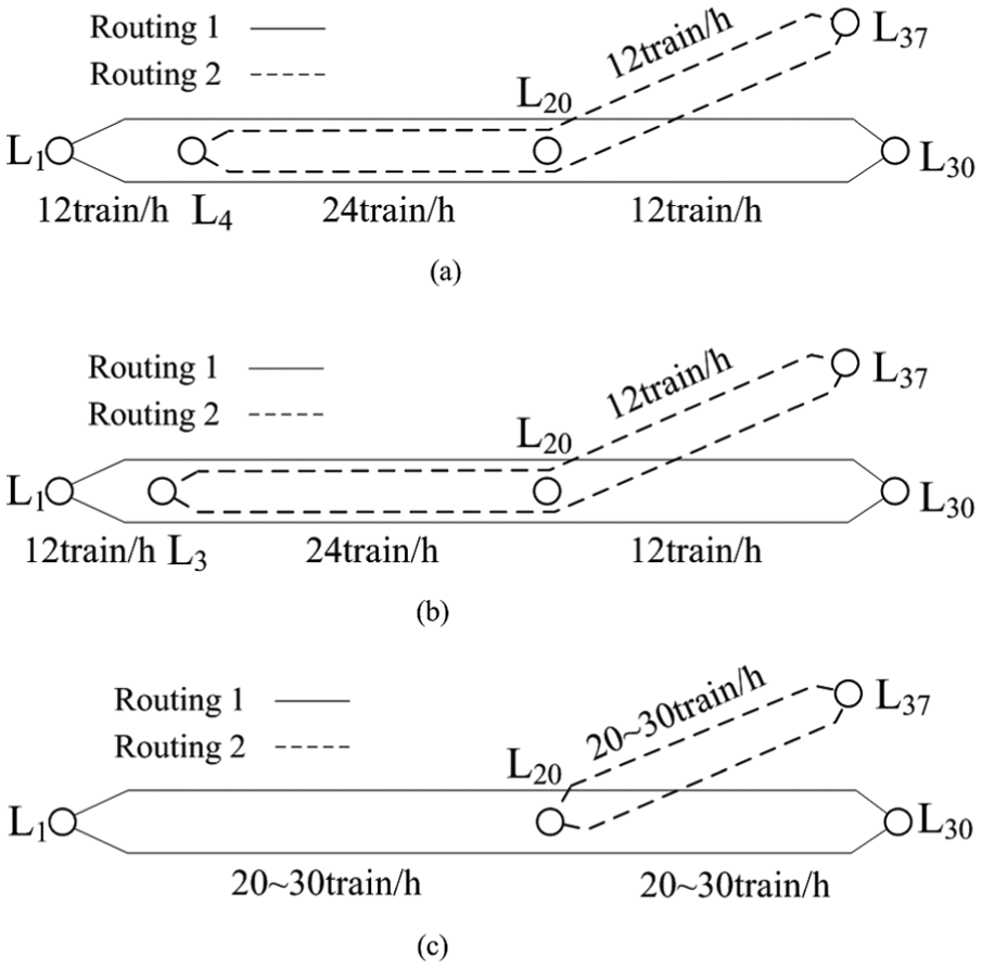
The typical forms of multi-routing planning of Y-type line include separate operation, straight-through operation, and integrated operation which is a combination of the previous two forms. There are three combinations under two-routing planning, as shown in Figure 2(a)–(c). However, the combinations under three-routing planning are related to the relationships of the turn-backs of different routings. Thus, the combinations are numerous and several combinations are shown in Figure 2(d)–(f) because of the limitation of space.

Figure 2.

Typical multi-routing planning of Y-type line: (a) separate operation, (b) straight-through operation, (c) integrated operation under two-routing, (d) integrated operation 1 under three-routing, (e) integrated operation 2 under three-routing, and (f) integrated operation 3 under three-routing.

A routing planning with two routings is called two-routing planning, such as Figure 2(a)–(c); a routing planning with three routings is called three-routing planning, such as Figure 2(d)–(f). Most of the cases in use adopt a two-routing planning because the operation is not as complex as three-routing planning, but the diversity of three-routing planning may make it better meet the complex and unbalanced passenger demand, which may bring some additional profit to the passengers or the operator. Therefore, this article studied multi-routing planning of Y-type urban rail transit. The variables are the departure frequencies and the turn-back stations of the routings under the constraints of passenger demand and line condition, aiming at minimizing the passenger travel time and operator cost.

The article is organized as follows: sections “Description of the problem” and “Modeling” describe the problem and the modeling, respectively; section “Solution algorithm” describes the algorithm; section “Case study” studies on a case and section “Conclusion” concludes the article.

Modeling

The typical multi-routing planning of two-routing and three-routing are shown in Figures 3 and 4, respectively.

Figure 3.

Routing planning of two-routing.

Figure 4.

Routing planning of three-routing.

The routing covering all the stations on the trunk AOB is the trunk routing, called Routing 1; the routing covering the branch OC is the branch routing, called Routing 2. Routing 2 may covers some stations on AO, too; if there are three routings, the third one is a minor routing, called Routing 3. Therefore, Routing h is used to represent the routings, and h (h = 1, 2, 3) is the order number of the routing. The turn-back stations of Routing 1 are L₁ and L_m; the turn-back stations of Routing 2 are L_x and L_n; the turn-back stations of Routing 3 are L_y and L_z, and the departure frequency of Routing h is f_h (h = 1, 2, 3).

When f₃ ≠ 0, the planning is three-routing; when f₃ = 0, the planning is two-routing, and the planning is separate operation when L_x = L_b while straight-through operation when L_x = L₁, so the routing planning in Figure 4 can contain the variants shown in Figure 2. The major variables, parameters, and notations used in this article are shown in Tables 1 –3, respectively.

Table 1.

Variables and definitions.

Variables	Definition
L_x	Unknown turn-back station of Routing 2; decision variable
L_y	Unknown turn-back station of Routing 3 with a smaller order number; decision variable
L_z	Unknown turn-back station of Routing 3 with a larger order number; decision variable
f_h	Departure frequencies of Routing h (h = 1, 2, 3) in the research period T, train/h; decision variable

Table 2.

Parameters and definitions.

Parameters	Definition
L_k	Station k, in which k is the order number of the station
L_b	Node station of the Y-type line
L_m	Terminal station of the trunk line
L_n	Terminal station of the branch line
T	Research period, h
D_i,j	Passenger flow from Station L_i to Station L_j in the upward direction
$\bar{{ST}_{k}^{h}}$	Stop time of a train belonging to Routing h at Station L_k, s
ST_max	Lower limit of $\bar{{ST}_{k}^{h}}$ , s
ST_min	Upper limit of $\bar{{ST}_{k}^{h}}$ , s
R_h	Operating distance of Routing h for one trip, km
a_k	Number of upward passengers boarding at station L_k in T
q_k	Upward passenger flow on the section between Stations L_k and L_k+₁ in T
$β_{h}^{k, k + 1}$	0–1 Decision variable, the value is 1 when Routing h covers the section between Station k and Station k + 1, and 0 otherwise
n_v	Seating capacity of a train with fixed formation
$δ$	Average passenger boarding time, s
$η$	Load factor of the trains
$ϕ$	Weight of objective Z₁’s standard value
t_o	Average walking time for transferring, s
I_min	Ruled minimum headway, s
t_i,j	Running time of a train from Station L_i to Station L_j, s
P_g	Passengers are divided into groups according to their available choice of routings
$λ_{h}^{g}$	Sharing rate of Routing h for passenger group P_g
$x_{h}^{g}$	0–1 Decision variable, the value is 1 when Routing h bears P_g, and 0 otherwise

Table 3.

Notations and definitions.

Notations	Definition
H	Order number of routings. Routing 1, Routing 2, and Routing 3 are, respectively, expressed as $h = 1$ , $h = 2$ , and $h = 3$
Z ₁	Objective 1, passenger travel time in T, s
Z ₂	Objective 2, train operating distance in T, km
CW	Passenger waiting time in T, s
CV	Passenger in-vehicle time in T, s
CT	Passenger transfer time in T, s
S	Set of stations with turn-back tracks

The multi-routing planning of Y-type line is complex, so the following assumptions were used to simplify the problem:

The passenger flow of the trunk is usually larger than the branch, which is easier to show the characteristic of unbalanced. Thus, the minor routing (Routing 3) was assumed on the trunk line if it existed.

Passengers would not choose routings with transfers unless they had to.

The trains’ formation was fixed.

The arrival of passengers was assumed to follow uniform distribution under large passenger flow with short intervals.

Passengers boarded and alighted at the stations simultaneously, and the boarding process was slower. Thus, the stop time of a train at each station was assumed to be equal to the boarding time with an upper limit and a lower limit.

Considering the saturated capacity of a subway at the peak hour, the departure frequencies of different routings were assumed to have multiple relationships with each other, which could ensure balanced headways under a certain level of service.

The designing of routing planning affects the service quality for the passengers and the operational cost of the operator. Therefore, this article proposed a model considering both the travel time of the passengers and the operating distance of the trains to represent service quality and operational cost. Also, the constraints such as turn-back tracks of stations, transport capacity and passenger demand, and tracking interval were considered. Finally, the optimal solutions of routing planning were obtained.

Passenger travel time

The passenger travel time was composed of waiting time, in-vehicle time, and transfer time. Waiting time was the product of passenger flow and average waiting time; in-vehicle time was the product of passenger flow and section running time, station stop time; transfer time was the product of transfer passenger flow and average transfer time. The passenger travel time is expressed as follows

Z_{1} = CW + CV + CT

(1)

In which Z₁ is the passenger travel time (s), CW is the passenger waiting time (s), CV is the passenger in-vehicle time (s), and CT is the passenger transfer time (s).

Waiting time

The location of a station determines the service frequencies for the passengers at the station, for example, in Figure 3, Stations L₁−L_x and L_b−L_m are only covered by Routing 1, Stations L_b−L_n are only covered by Routing 2, and Stations L_x−L_b are covered by both routings. For ease of expression, the Y-type line is divided into at most six passenger segments shown in Figure 5 according to the location of turn-back stations, and this way of division can cover other situations, such as when L_x = L_b, it would be separate operation, and Segment 2 no longer exists; when L_x = L₁, it would be straight-through operation, and Segment 1 no longer exists. The passenger flow from Segment 1 to Segment 2 is expressed as $c_{12} = \sum_{i = 1}^{x - 1} \sum_{j = x}^{b} D_{i, j}$ , and so on.

Figure 5.

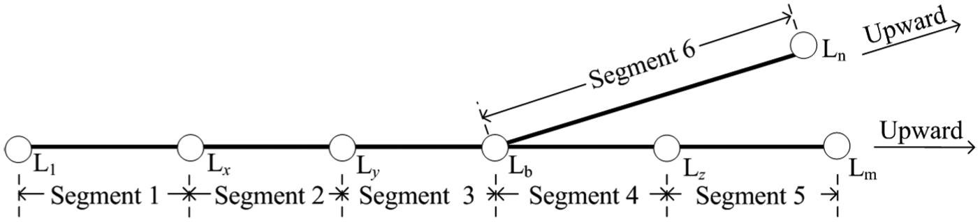
Segments divided by turn-back stations.

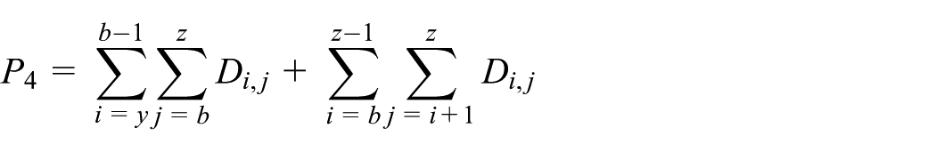
A passenger’s choice for the routings is dependent on his or her OD (origin station and destination station), such as passengers from Segment 1 to Segment 6 in Figure 5 need to transfer from Routing 1 to Routing 2, while passengers from Segment 2 to Segment 6 only need to catch Routing 2. According to Assumption 2, passengers were divided into groups named P_g: P₁ needed to catch Routing 1; P₂ needed to catch Routing 2; P₃ could catch Routing 1 or Routing 2; P₄ could catch Routing 1 or Routing3; P₅ could catch Routing 1, Routing 2, or Routing 3. In this section, the waiting time of the passengers who need to transfer only accounts for the waiting time for the first routing they catch, and the waiting time for the routing after transferring would be calculated in section “Tranfer time”. Thus, the expressions of P_g are as follows

\begin{matrix} P_{1} = \sum_{i = 1}^{x - 1} \sum_{i + 1}^{n} D_{i, j} + \sum_{i = x}^{y - 1} \sum_{j = z}^{m} D_{i, j} + \sum_{i = y}^{z} \sum_{j = z + 1}^{m} D_{i, j} \\ + \sum_{i = z + 1}^{m - 1} \sum_{j = i + 1}^{m} D_{i, j} + \sum_{i = b}^{n} \sum_{j = z + 1}^{m} D_{i, j} \end{matrix}

P_{2} = \sum_{i = x}^{m} \sum_{j = m + 1}^{n} D_{i, j} + \sum_{i = m + 1}^{n - 1} \sum_{j = i + 1}^{n} D_{i, j}

P_{3} = \sum_{i = x}^{y} \sum_{j = x + 1}^{b} D_{i, j}

P_{4} = \sum_{i = y}^{b - 1} \sum_{j = b}^{z} D_{i, j} + \sum_{i = b}^{z - 1} \sum_{j = i + 1}^{z} D_{i, j}

P_{5} = \sum_{i = y}^{b - 1} \sum_{j = i + 1}^{b} D_{i, j}

According to Assumption 3, the average waiting time could be calculated as half of the headway,⁹ which was the interval between two successive trains. Thus, passenger waiting time was calculated as follows

CW = \sum_{h = 1}^{3} \sum_{g = 1}^{5} (λ_{h}^{g} \cdot P_{g} \cdot T / 2 f_{h})

(2)

λ_{h}^{g} = \frac{x_{h}^{g} \cdot f_{h}}{\sum_{h = 1}^{3} \sum_{g = 1}^{5} (x_{h}^{g} \cdot f_{h})}

(3)

In which $λ_{h}^{g}$ is the sharing rate of Routing h for passenger group P_g; $x_{h}^{g}$ is a 0–1 decision variable, the value was 1 when Routing h could bear P_g, and 0 otherwise.

In-vehicle time

The in-vehicle time was composed of running time between the stations and passengers’ waiting time when the train stopped at the stations. The former was the product of the sections’ running time and the sections’ passenger flow, and the latter was the product of the passenger flow passing the stations and trains’ stop time at the stations.¹⁷ According to Assumption 4, the stop time at the stations was related to the number of passengers boarding with an upper limit and a lower limit, and the passengers boarding a train was related to passenger flow, share rate, and departure frequencies of the routings. The in-vehicle time after transferring of the transfer passengers is calculated in the same way. The passengers were assumed to have the same choice ratio for each gate. Therefore, the passenger in-vehicle time was expressed as follows

CV = \sum_{i = 1}^{n} \sum_{j = i + 1}^{n} (D_{i, j} \times t_{i, j}) + δ \sum_{k = 1}^{n} \sum_{h = 1}^{3} \sum_{g = 1}^{5} (λ_{h}^{g} \cdot q_{k}) \times \bar{{ST}_{k}^{h}}

(4)

\bar{{ST}_{k}^{h}} = \frac{(λ_{h}^{g} \cdot a_{k})}{4 n_{v} f_{h}}

(5)

a_{k} = {\begin{matrix} \sum_{j = k + 1}^{n} D_{k, j}, k \in [1, b] \cup [m + 1, n) \\ \sum_{j = k + 1}^{m} D_{k, j}, k \in [b + 1, m) \end{matrix}

(6)

In which t_i,j is the running time from Stations L_i to L_j (s); $δ$ is the average passenger boarding time (s); q_k is the passenger flow on the section between Stations L_k and L_k₊₁ in period T; $\bar{{ST}_{k}^{h}}$ is the stop time at Station L_k of a train belonging to Routing h (s); ST_max and ST_min are the lower limit and the upper limit of $\bar{{ST}_{k}^{h}}$ , respectively (s); n_v is the seating capacity of a train with fixed formation, and every carriage had four gates; a_k is the number of upward passengers boarding at Station L_k in period T.

Transfer time

The passenger transfer time was composed of walking time and waiting time for transferring which could be calculated approximately by half of the aimed routing’s headway, so the passenger transfer time could be calculated as follows

\begin{matrix} CT = t_{0} \cdot (\sum_{i = 1}^{L_{x}} \sum_{j = m + 1}^{n} D_{i, j} + \sum_{i = b + 1}^{m} \sum_{j = m + 1}^{n} D_{i, j} + \sum_{i = m + 1}^{n} \sum_{j = b + 1}^{m} D_{i, j}) \\ + (\sum_{i = 1}^{L_{x}} \sum_{j = m + 1}^{n} D_{i, j} + \sum_{i = b + 1}^{m} \sum_{j = m + 1}^{n} D_{i, j}) \cdot T / 2 f_{2} \\ + \sum_{i = m + 1}^{n} \sum_{j = b + 1}^{z} D_{i, j} \cdot T / 2 (f_{1} + f_{3}) + \sum_{i = m + 1}^{n} \sum_{j = z + 1}^{m} D_{i, j} \cdot T / 2 f_{1} \end{matrix}

(7)

In which t_o is the average walking time for transferring (s).

Train operating distance

Suppose the vehicles were sufficient, the operating distance could stand for the operator cost which was expressed as follows. The train operating distance was the product of the departure frequencies and the distance of the routes, and the latter one was related to the locations of turn-backs. It should be noted that the deadheading of the trains from the depot to the nearer turn-back stations of the routings was quite small compared to the operating distance of the trains, so the deadheading distance was ignored

Z_{2} = \sum_{h = 1}^{3} (f_{h} \cdot R_{h})

(8)

In which Z₂ is the trains’ operating distance (km); R_h is one trip’s operating distance of Routing h (km).

Multi-objective model

As the passenger travel time and train operating distance have different unites of measurement, they could be transformed into standard values by formula (10) to be nondimensional. Then the objectives were given weighted values to turn the model into a single-objective model¹⁸ by formula (9)

min Z = ϕ {\bar{Z}}_{1} + (1 - ϕ) {\bar{Z}}_{2} (0 \leq ϕ \leq 1)

(9)

$s . t .$

{\bar{Z}}_{θ} = \frac{Z_{θ} - Z_{θ min}}{Z_{θ max} - Z_{θ min}} \in [0, 1] (θ = 1, 2)

(10)

Formulas (1)–(7)

\sum_{h = 1}^{3} f_{h} \leq \frac{T}{I_{\min}}

(11)

\begin{matrix} (f_{2} = a_{1} f_{1} \cap f_{3} = a_{2} f_{1}) \cup (f_{1} = a_{1} f_{2} \cap f_{3} = a_{2} f_{1}) \\ (a_{1} \in N *, a_{2} \in N) \end{matrix}

(12)

f_{min} \leq \sum_{h = 1}^{3} (β_{h}^{k, k + 1} \cdot f_{h})

(13)

λ_{h}^{g} \cdot q_{k} \leq β_{h}^{k, k + 1} \cdot f_{h} \cdot n_{v} \cdot η

(14)

L_{x}, L_{y}, L_{z} \in S

(15)

L_{x} \leq L_{b}

(16)

S T_{min} \leq \bar{{ST}_{k}^{h}} \leq S T_{max}

(17)

$ϕ$ is the weight of $Z_{1}$ , and it’s larger when Z₁ is more important; ${\bar{Z}}_{θ}$ , $Z_{θ max}$ , and $Z_{θ min}$ are the standard value, the maximum value, and the minimum value of the objective, respectively; formula (11) ensured that the headway of the trains on every section was larger than the ruled minimum headway I_min; formula (12) ensured that the departure frequencies satisfied Assumption 6 to decrease the unbeneficial effect on the capacity of the line; $f_{min}$ is the ruled minimum departure frequency on each section; $β_{h}^{k, k + 1}$ is a 0–1 variance, the value was 1 when Routing h covered the section between Stations L_k and L_k+₁, otherwise 0; thus formula (13) ensured that the departure frequency on each section of the line was larger than the ruled one; formula (14) ensured that the transport capacity of each routing on each section was larger than its passenger demand under a certain load factor $η$ ; n_v is the sitting capacity of a train with fixed formation; formula (15) ensured that the turn-back stations were chosen from the stations with turn-back tracks; formula (16) ensured that each station on the line was covered by at least one routing; formula (17) ensured that the stop time of a train at a station was in a certain range according to Assumption 5.

Solution algorithm

The proposed model involved a complicated mixed-integer nonlinear programming problem, so the optimal solutions could not be easily obtained by adopting polynomial algorithms when the scale of Y-type line expanded. However, genetic algorithm (GA) is suitable for solving multivariable complex problems with multiple parameters, and it is widely applied in solving routing planning problems due to its extensive generality, strong robustness, high efficiency, and practical applicability. Therefore, this study adopted GA to solve the problem, and the key steps were designed as follows:

1. Chromosome encoding. In this study, 0–1 binary encoding was used. The genes for chromosomes in GA were the decision variables of the model, including order number of the unknown turn-back stations of Routing 2 (L_x), the unknown turn-back stations of Routing 3 (L_y and L_z), and the departure frequencies (f₁, f₂, f₃) of the routings. Considering the maximum frequency is 30 train/h, the number of genes for the frequency of a routing was set to be five. The number of stations on the trunk line is usually less than 30, so the number of genes for the order number of a turn-back station was set to be five. Thus, the expression of a chromosome is shown in Figure 6.

2. Chromosome decoding. The chromosomes of turn-back stations and departure frequencies were decoded into real solutions. This step was repeated until the solution satisfied all constraints including formulas (11)–(17) and re-encoded the real solution to 0–1.

3. Fitness calculation. It was necessary to transform the objective formula (9) into a maximization problem since the GA was designed to solve maximization problems. Given a certain weight value chosen from [0, 1.0] in the model, as the maximum value of the objective is 1.0, the fitness function was equal to 1.0 minus the chromosome’ objective Z, expressed as follows

F (X) = 1 - Z (X)

(18)

In which X is the order number of the chromosome in the population, and Z(X) is the objective of the chromosome calculated by formula (9).

4. Crossover and mutation operations. Two chromosomes with the largest fitness were recorded to operate single-point crossover and single-point mutation. The optimal solutions under two-routing and three-routing were obtained under the certain weight value. The algorithm won’t terminate until all the optimal solutions under each weight value have been obtained; otherwise, record them and recalculate with a new weight value again.

Figure 6.

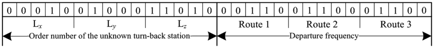
Expression of chromosomes.

Other detailed steps or approaches of GA were similar to the standard GA.

Case study

Figure 7 shows the layout of a Y-type urban rail transit line. The node station is $L_{7}$ , and $b = 20$ , $m = 10$ , and $n = 7$ ; there are 37 stations in total. Considering the modernization of the tracks, it was assumed that all the stations had turn-back tracks, so any station could be chosen as a turn-back location of a routing. The routings were assumed to adopt station-behind turn-back, so when Routing h turned back at station k, the routing covered the station. Figure 8 shows passenger flow on each section in peak hour, and the research period T is 7:30–8:30 a.m. in morning peak hour. The passenger volume was obtained from a pre-feasibility study of a line in China. According to the actual situation of the line, the parameters adopted are shown in Table 4.

Figure 7.

Layout of an urban rail transit line.

Figure 8.

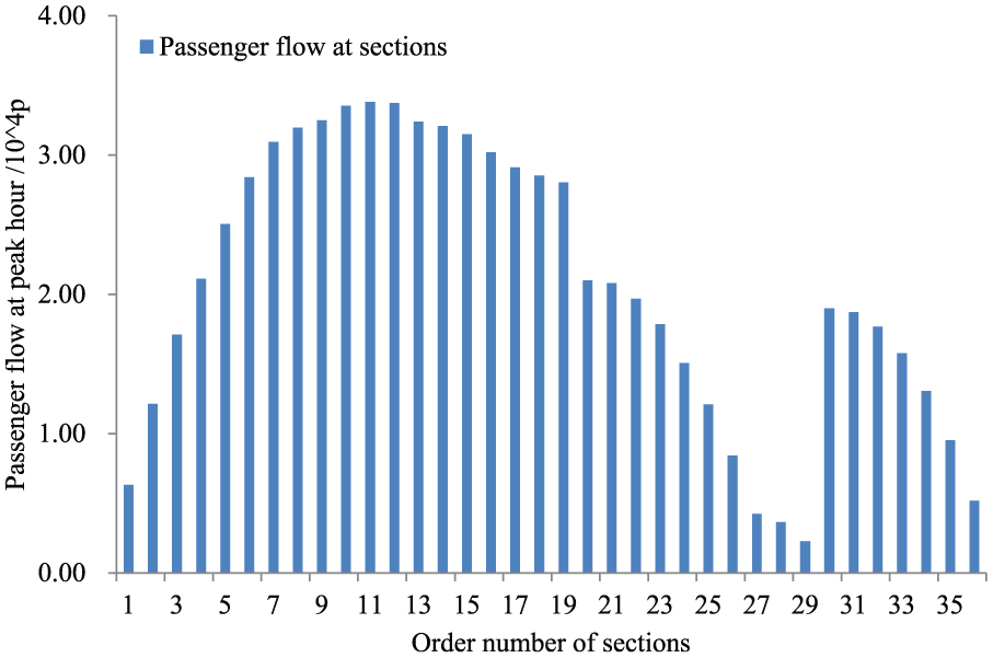
Passenger flow of each section in morning peak hour (7:30–8:30 a.m.).

Table 4.

Value of parameters.

Parameters	n_v	I_min	$f_{min}$	$η$	ST_min	ST_max	$δ$	t_o
Value	1860p	120 s	6 train/h	1.0	15 s	45 s	1.51 s	300 s

Result analysis

According to the proposed model, the weight value of the passenger travel time and the form of multi-routing planning affected the optimal solutions. Thus, this article calculated the optimal solutions under the form of three-routing and two-routing, respectively, with the weight increased from 0 to 1.0. The results are shown in Tables 5 and 6, and the forms of the routing planning are shown in Figures 9 and 10.

Table 5.

Optimal solutions of three-routing planning with different weight values.

$ϕ$	Order number of turn-back stations			Departure frequencies (train/h)			Train operating distance (km)	Passenger travel time (10⁴ s)	Passenger waiting time (10⁴ s)	Passenger in-vehicle time (10⁴ s)	Passenger transfer time (10⁴ s)	$Z_{1}$	$Z_{2}$	Z
$ϕ$	Routing 1	Routing 2	Routing 3	$f_{1}$	$f_{2}$	$f_{3}$	Train operating distance (km)	Passenger travel time (10⁴ s)	Passenger waiting time (10⁴ s)	Passenger in-vehicle time (10⁴ s)	Passenger transfer time (10⁴ s)	$Z_{1}$	$Z_{2}$	Z
0	(1, 30)	(3, 37)	(20, 27)	7	14	14	1026.1	6013.0	87.3	5538.8	386.9	0.84	0.02	0.02
0.1	(1, 30)	(3, 37)	(20, 27)	7	14	14	1026.1	6013.0	87.3	5538.8	386.9	0.84	0.02	0.10
0.2	(1, 30)	(2, 37)	(8, 26)	6	12	12	1065.2	5888.4	93.1	5383.4	411.9	0.56	0.07	0.16
0.3	(1, 30)	(2, 37)	(2, 26)	6	12	12	1155.3	5767.3	78.2	5277.2	411.9	0.28	0.17	0.21
0.4	(1, 30)	(2, 37)	(2, 30)	6	12	12	1260.9	5660.7	46.6	5272.6	341.5	0.04	0.30	0.19
0.5	(1, 30)	(2, 37)	(2, 30)	6	12	12	1260.9	5660.7	46.6	5272.6	341.5	0.04	0.30	0.17
0.6	(1, 30)	(1, 37)	(2, 30)	6	12	12	1306.1	5643.9	33.6	5270.0	340.3	0.00	0.35	0.14
0.7	(1, 30)	(1, 37)	(2, 30)	6	12	12	1306.1	5643.9	33.6	5270.0	340.3	0.00	0.35	0.11
0.8	(1, 30)	(1, 37)	(2, 30)	6	12	12	1306.1	5643.9	33.6	5270.0	340.3	0.00	0.35	0.07
0.9	(1, 30)	(1, 37)	(2, 30)	6	12	12	1306.1	5643.9	33.6	5270.0	340.3	0.00	0.35	0.04
1.0	(1, 30)	(1, 37)	(2, 30)	6	12	12	1306.1	5643.9	33.6	5270.0	340.3	0.00	0.35	0.00

Table 6.

Optimal solutions of two-routing planning with different weight values.

$ϕ$	Turn-back stations			Departure frequencies (train/h)			Train operating distance (km)	Passenger travel time (10⁴ s)	Passenger waiting time (10⁴ s)	Passenger in-vehicle time (10⁴ s)	Passenger transfer time (10⁴ s)	$Z_{1}$	$Z_{2}$	Z
$ϕ$	Routing 1	Routing 2	Routing 3	$f_{1}$	$f_{2}$	$f_{3}$	Train operating distance (km)	Passenger travel time (10⁴ s)	Passenger waiting time (10⁴ s)	Passenger in-vehicle time (10⁴ s)	Passenger transfer time (10⁴ s)	$Z_{1}$	$Z_{2}$	Z
0	(1, 30)	(4, 37)	−	12	12	−	1009.0	5972.1	41.1	5518.5	412.4	0.75	0.00	0.00
0.1	(1, 30)	(3, 37)	−	12	12	−	1009.0	5967.4	38.9	5517.0	411.6	0.74	0.00	0.07
0.2	(1, 30)	(3, 37)	−	12	12	−	1009.0	5967.4	38.9	5517.0	411.6	0.74	0.00	0.15
0.3	(1, 30)	(3, 37)	−	12	12	−	1009.0	5967.4	38.9	5517.0	411.6	0.74	0.00	0.22
0.4	(1, 30)	(3, 37)	−	12	12	−	1009.0	5967.4	38.9	5517.0	411.6	0.74	0.00	0.29
0.5	(1, 30)	(20, 37)	−	20	20	−	1233.3	5821.1	18.1	5333.6	469.4	0.40	0.27	0.33
0.6	(1, 30)	(20, 37)	−	20	20	−	1233.3	5821.1	18.1	5333.6	469.4	0.40	0.27	0.35
0.7	(1, 30)	(20, 37)	−	23	23	−	1418.3	5770.4	13.7	5304.8	452.0	0.29	0.49	0.35
0.8	(1, 30)	(20, 37)	−	28	28	−	1726.6	5714.4	9.2	5274.0	431.2	0.16	0.85	0.30
0.9	(1, 30)	(20, 37)	−	30	30	−	1850.0	5699.6	8.0	5266.7	424.8	0.13	1.00	0.21
1.0	(1, 30)	(20, 37)	−	30	30	−	1850.0	5699.6	8.0	5266.7	424.8	0.13	1.00	0.13

Figure 9.

Optimal solution of three-routing planning: (a) ϕ = 0–0.1, (b) ϕ = 0.2, (c) ϕ = 0.3–0.5, and (d) ϕ = 0.4–1.0.

Figure 10.

Optimal solution of two-routing planning: (a) ϕ = 0, (b) ϕ = 0.1–0.4, and (c) ϕ = 0.5–1.0.

Figure 9 shows that when the weight of the passenger travel time $ϕ$ increases, the passenger travel time decreases while the train operating distance increases. When $ϕ$ increases from 0 to 0.2, the turn-back stations of Routing 2 and Routing 3 change to make the routings longer, and the departure frequencies of the routings decrease to meet the constraint of the minimum track interval; when $ϕ$ increases from 0.3 to 1.0, the turn-back stations of Routing 2 and Routing 3 change to make both routings longer under the same departure frequencies, leading to less passenger travel time and more train operating distance.

Figure 10 shows that when the weight of the passenger travel time $ϕ$ increases from 0 to 0.4, Routing 2 becomes longer under the same departure frequencies, leading to less passenger travel time and more train operating distance; when $ϕ$ increases from 0.4 to 1.0, Routing 2 becomes shorter to turn the straight-through operation to separate operation, so the frequencies of both routings could increase to 30 train/h which is the maximum frequency, leading to less passenger travel time and more train operating distance.

Comparison of three-routing planning and two-routing planning

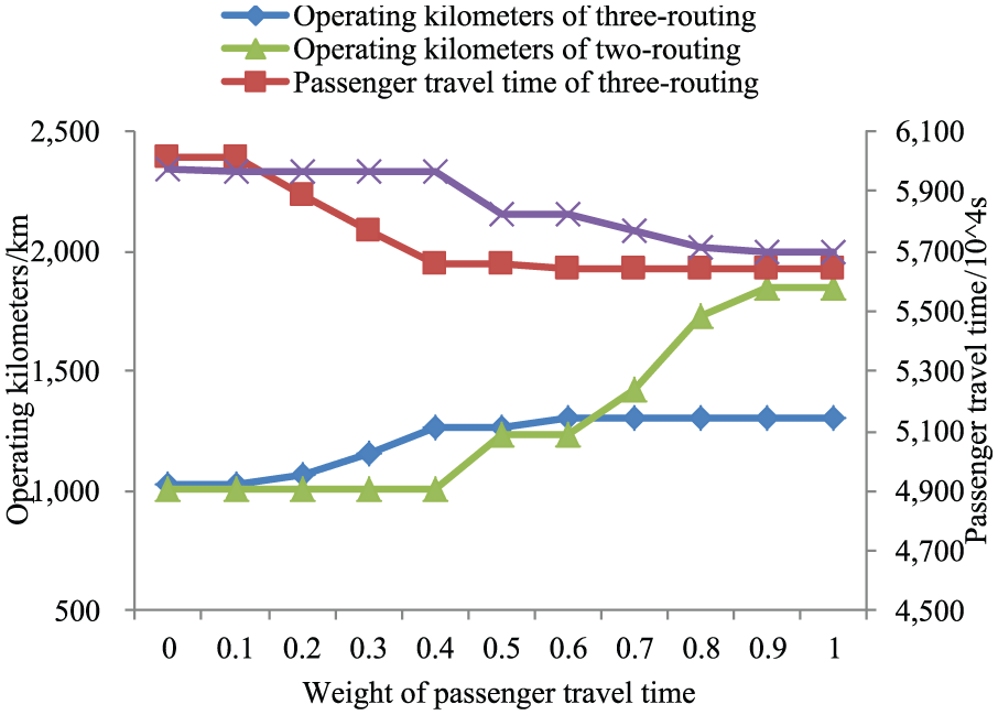
To discuss the influence of different routing planning and weight values on the objectives, passenger travel time (Z₁) and train operating distance (Z₂) of the optimal solutions under the form of three-routing and two-routing planning with different weight values of passenger travel $ϕ$ are shown in Figure 11, respectively.

Figure 11.

Objectives of the optimal solutions under the form of three-routing and two-routing.

Figure 11 shows the following:

When the weight of the passenger travel time increases, the passenger travel time of three-routing planning and two-routing planning decreases, while the train operating distance increases.

When the weight of the passenger travel time increases from 0.4 to 1.0, the operating distance of two-routing planning increases sharply while the passenger travel time decreases relatively flat. At the same time, the routing planning changes from Figure 9(b) to Figure 9(c), and the departure frequencies of both routings increase from 12 train/h to 20–30 train/h, leading to a quick increase in the train operating distance. However, the passenger flow of some stations on the line are relatively small because of the unbalanced characteristic, which makes the increase in the train operating distance more obvious than the decrease in the passenger travel time. Therefore, it is not necessary to increase the weight of the passengers too much because the cost increases much more.

When the weight of the passenger travel time ranges from 0.7 to 0.8, both objectives of three-routing planning are better than two-routing planning. Routing 2 in the three-routing planning does not cover L₁−L₂, so the passengers aimed to the branch boarding at Station 1 need to transfer and the passenger walking time for transferring increased a little. However, the frequencies of L₂₀−L₃₀ and L₂₀−L₃₇ are 18 and 12 train/h in the three-routing planning and 15 and 15 train/h in the two-routing planning, respectively; as more passengers travel on the trunk line, the three-routing planning can decrease the waiting time for transferring, and the degree of decrease is larger than the degree of increase in the walking time mentioned previously. Therefore, three-routing planning can better copy with the characteristics of the passengers’ demand by increasing the departure frequencies on sections with larger passenger flow while decreasing departure frequencies on sections with smaller passenger flow.

To discuss the influence of different routing planning and weight values on the comprehensive objective Z in formula (9), the comparison of Z under three-routing and two-routing with different weight values is shown in Figure 12. Z was the weighted sum of the standard value of the two objectives, so Z had no dimension, and the range of Z was [0, 1]. The values were obtained from Tables 5 and 6.

Figure 12.

Weighted objective of the optimal routing planning under three-routing and two-routing.

Figure 12 shows the following:

When the weight of the travel time increases, the weighted objective of three-routing planning and two-routing both show decreasing trends after the first increase.

The smaller the weighted objective, the better the optimal solution. Thus, when ϕ = 0.1–0.6, the optimal solution is a two-routing planning; when ϕ = 0.7–1.0, the optimal solution is a three-routing planning. Therefore, three-routing planning is more suitable when the passenger travel time is more important while two-routing planning is more suitable when the train operating distance is more important.

Conclusion

In this study, a multi-routing planning design model of Y-type urban rail transit aimed at minimizing the passenger travel time and train operating distance was proposed, and the multi-objective model was turned into a single-objective model by giving the weight values of the objectives. The model optimized the departure frequencies and the locations of turn-backs of the routings considering the passenger demand and layout of the line. A GA was designed to obtain optimal solutions. A case was used to find out the effects of the variables on the objectives, and the standard values of the two objectives were given different weight values to discuss the change in routing planning. Also, the applicability of three-routing planning and two-routing planning was analyzed.

When the weight of the passenger travel time is lower, the optimal solution is two-routing planning; when the weight is higher, the optimal solution is three-routing planning.

When the weight of the passenger travel time increases, the passenger travel time of both three-routing planning and two-routing planning decreases while the train operating distance of both increases.

When the weight of the passenger travel time reaches to a certain value, three-routing planning can better meet the unbalanced passenger flow than two-routing planning by increasing the departure frequencies on sections with large passenger demand while decreasing those with small passenger demand.

This article did not consider the operational complexity of three-routing planning and the impact on the number of vehicles, which will be the focus of future research.

Footnotes

Academic Editor: António Mendes Lopes

Declaration of conflicting interests

The author(s) declared no potential conflicts of interest with respect to the research, authorship, and/or publication of this article.

Funding

The author(s) disclosed receipt of the following financial support for the research, authorship, and/or publication of this article: This research was supported by National Natural Science Foundation of China (71390332) and National Natural Science Fund Projects (71571061, 71201007).

References

Vuchic

VR.

Urban transit: operation, planning and economics. Hoboken, NJ: John Wiley & Sons, Inc., 2004.

Furth

PG.

Short turning on transit routes. Transp Res Record 1987; 1108: 42–52.

Furth

Day

FB.

Transit routing and scheduling strategies for heavy demand corridors. Transp Res Record 1985; 1011: 23–26.

Ceder

Optimal design of transit short-turn trips. Transp Res Record 1989; 1221: 8–22.

Ceder

Stern

HI.

Deficit function bus scheduling with deadheading trip insertions for fleet size reduction. Transport Sci 1981; 15: 338–363.

Nesheli

Ceder

A robust, tactic-based, real-time framework for public-transport transfer synchronization (The international symposium on transportation and traffic theory). Transp Res Procedia 2015; 9: 246–268.

Vijayaraghavan

TAS

Anantharamaiah

. Fleet assignment strategies in urban transportation using express and partial services. Transport Res A: Pol 1995; 29: 157–171.

Cortés

Jara-Díaz

Tirachini

Integrating short turning and deadheading in the optimization of transit services. Transport Res A: Pol 2011; 45: 419–434.

Tirachini

Cortés

Jara-Díaz

Optimal design and benefits of a short turning strategy for a bus corridor. Transportation 2011; 38: 169–189.

10.

Site

Filippi

Service optimization for bus corridors with short-turn strategies and variable vehicle size. Transport Res A: Pol 1998; 32: 19–38.

11.

Canca

Barrena

Laporte

. A short-turning policy for the management of demand disruptions in rapid transit systems. Ann Oper Res. Epub ahead of print 3 July 2014. DOI: 10.1007/s10479-014-1663-x.

12.

Jannson

JO.

A simple bus line model for optimization of service frequency and bus size. J Transp Econ Policy 1980; 14: 53–80.

13.

Chen

Zhou

. Study on the algorithm for train operation adjustment based on ordinal optimization. Adv Mech Eng 2013; 5: 175347.

14.

Riejos

FAO

Barrena

Ortiz

JDC

. Analyzing the theoretical capacity of railway networks with a radial-backbone topology. Transport Res A: Pol 2015; 84: 83–92.

15.

Song

Study on operation plans of Shanghai Mingzhu transit system network. J Tongji Univers 2003; 31: 682–686 (in Chinese).

16.

Fioole

Kroon

Maróti

. A rolling stock circulation model for combining and splitting of passenger trains. Eur J Oper Res 2006; 174: 1281–1297.

17.

Freyss

Giesen

Muñoz

JC.

Continuous approximation for skip-stop operation in rail transit. Transport Res C: Emer 2013; 36: 419–433.

18.

Cui

Chen

S-K

Liu

J-F.

Layout optimization of the feeder bus routings connecting subways at bus stops. J Transp Syst Eng Inf Technol 2013; 13: 176–183 (in Chinese).

Multi-routing planning design of Y-type urban rail transit

Abstract

Keywords

Introduction

Description of the problem

Modeling

Passenger travel time

Waiting time

In-vehicle time

Transfer time

Train operating distance

Multi-objective model

Solution algorithm

Case study

Result analysis

Comparison of three-routing planning and two-routing planning

Conclusion

Footnotes

Declaration of conflicting interests

Funding

References