Particle swarm optimization used with proportional–derivative control to analyze nonlinear behavior in the atomic force microscope

Abstract

An investigation of nonlinear probe behavior in an atomic force microscope, caused by different excitation frequencies, was carried out as well as an analysis and subsequent regulation using particle swarm optimization in combination with proportional–derivative control. The dynamic behavior was resolved by numerical analysis using the atomic force microscope probe governing equations and the properties were examined using phase portrait, bifurcation diagrams, Poincaré maps, and the maximum Lyapunov exponent. The results show that excitation frequency ratio can actuate periodic, sub-harmonic, and chaotic behavior in the system under certain conditions. A proportional–derivative controller was employed to control the chaos, and particle swarm optimization was used to find the proportional–derivative parameters. Integral absolute error was used to evaluate the quality of the parameters for the performance indicator. The generation of nonlinear behavior and a chaotic state may be effectively suppressed to improve the stability and performance of an atomic force microscope system.

Introduction

The atomic force microscope (AFM) is a scanning probe microscope (SPM), which can image almost any kind of surface, such as glass, ceramics, polymers, and even biological materials. AFM is used extensively in materials science, biotechnology, micro-electro mechanical systems, biochemical technology, and many others.

AFM could be used in three different operational modes including contact, non-contact, and tapping mode. The non-contact mode holds the probe, on the cantilever, just above the surface of the specimen by utilizing the attractive forces between the atoms of the specimen and the probe tip. No contact is made between the specimen and the probe. For the instrument of tapping mode, the cantilever is driven by an oscillator to vibrate at a frequency close to resonance. Nonlinear interaction between the probe tip and the surface of the sample influence the dynamic behavior of the cantilever. For a dynamic realization of AFM, the intermolecular force between the probe on the cantilever and the sample is utilized to analyze material properties of the sample. Measurements of the probe deflections can be used to construct an optical image of the specimen surface to examine its physical properties.

Burnham et al.^1,2 investigated the dynamic behavior of the microcantilever of an AFM and found that the cantilever could show chaotic behavior under certain conditions. Ashhab et al. ³ used the Melnikov method to analyze and simulate the dynamic behavior of microcantilevers. Lee et al. ⁴ proposed interaction between nonlinear dynamic behavior and the effect of van der Waals force. Rutzel et al. ⁵ demonstrated that the Lennard-Jones (LJ) potential drives the nonlinear dynamic behavior of AFM probes.

Solares and Chawla ⁶ implemented a trimodal tapping-mode atomic force microscope (AFM) imaging scheme for ambient air with which it is possible to simultaneously acquire topographical and phase and frequency shift contrast images. By implementing this method, they had identified conditions, such as very low fundamental amplitude setpoints and very low oscillation amplitudes for the higher eigenmodes, for which the stability of the imaging process can be compromised. Also, numerical simulations are used to gain insight into the changes in the frequency response of the higher eigenmodes in bimodal and trimodal operation for different levels of sample stiffness, tip–sample dissipative forces, and oscillation amplitudes for each of the eigenmodes and cantilever rest positions above the surface. The simulation results are in general agreement with experimental observations.

Sahin et al. ⁷ studied the dynamic force microscopy (DFM) and atomic force microscopy (AFM) in which force-sensing cantilever probes a sample and thereby creates a topographic image of its surface. The simplest implementation uses the static deflection of the cantilever to probe the forces and the dynamic operation modes have been applied, which either work at a constant oscillation frequency or sense the amplitude variations caused by tip–sample forces.

Garcia and Proksch ⁸ focused on the bimodal force microscopy by dynamic force-based method with the capability of mapping simultaneously the topography and the nanomechanical properties of soft-matter surfaces and interfaces. The operating principle involves the excitation and detection of two cantilever eigenmodes. This method enables the simultaneous measurement of several material properties. A distinctive feature of bimodal force microscopy is the capability to obtain quantitative information with a minimum amount of data points. Furthermore, under some conditions the method facilitates the separation of the topography data from other mechanical and/or electromagnetic interactions carried by the cantilever response. They provided a succinct review of the principles and some applications of the method to map with nanoscale spatial resolution mechanical properties of polymers and biomolecules in air and liquid.

Borysov et al. ⁹ presented a theoretical framework for the dynamic calibration of the higher eigenmode parameters (stiffness and optical lever inverse responsivity) of a cantilever. This method is based on the tip–surface force reconstruction technique and does not require any prior knowledge of the eigenmode shape or the particular form of the tip–surface interaction. The calibration method proposed requires a single-point force measurement using a multimodal drive and its accuracy is independent of the unknown physical amplitude of a higher eigenmode.

From the past studies, it is known that AFM systems exhibit non-periodic or chaotic motion as the result of specific parameter under certain operating conditions within the probe tip vibrational amplitude, excitation frequency, and so forth. In order to understand and control when the AFM system occurs non-periodic motions and under what kind of operating conditions, the dynamic response of the AFM system will be analyzed and the dynamic behavior of probe tip will be examined and verified.

Also, particle swarm optimization (PSO)^10,11 combined with a proportional–derivative (PD) controller is used and developed to inhibit non-periodic motions like chaos in AFM system and to suppress the amplitude of the unstable vibrations. Meanwhile, the optimization parameters for control are found with PSO in a way that allows the system to suppress the generation of nonlinear behavior and quickly reach stability. It is anticipated that the results of this study will provide a valuable contribution to the design of AFM system and applied for use in a wide variety of industrial applications.

The remainder of this study is organized as follows. Section “Theoretical analysis” develops a mathematical model describing the time-dependent motions of the AFM system. Section “Numerical simulation and dynamic analysis” analyzed the behaviors of system by phase portrait, spectra analysis, bifurcation diagram, Poincaré maps, and Lyapunov exponents to obtain the whole dynamic characteristics of AFM system. Section “Chaos control” presents PSO combined with a PD controller to inhibit non-periodic motions efficiently and obtains the control simulation results to suppress the amplitude of the unstable vibrations. Finally, section “Conclusion” draws some brief conclusions.

Theoretical analysis

There exists an interactive force between the atoms on the probe tip and the atoms on the surface of the specimen. This means that the LJ potential equation may be utilized for calculation. The LJ potential model is the real contact mechanics in tapping-mode AFM system, and it represents a generic interaction of probe tip and surface qualitatively. It is considered that Ω, which is the ratio of the excitation frequency and the free resonance frequency of the cantilever, is close to the lowest frequency of the microcantilever. Under near-resonant forcing and in the absence of additional internal resonances, only one mode of the microcantilever is assumed to participate in the response. Thus, an AFM system can be simulated using a single degree of freedom in addition to non-dimensionalization. Thus, the dimensionless governing equation ⁵ is as follows

$${\stackrel{·}{X}}_1=X_2$$

(1)

$$\begin{array}{c}\multicolumn{1}{c}{{\stackrel{·}{X}}_2=-S_1{X}_2-X_1+S_2+\frac{S_3}{{(1-X_1-Z\sin (\Omega \tau ))}^8}}\\ \multicolumn{1}{c}{+\frac{S_4}{{(1-X_1-Z\sin (\Omega \tau ))}^2}+Z{\Omega }^2{S}_5\sin (\Omega \tau )}\end{array}$$

(2)

with initial conditions of

$$X_1=0$$

(3)

and

$$X_2=0$$

(4)

As shown in equation (2), X₁ indicates displacement of the probe tip, S₁ X₂ is the dimensionless damping term, S₂ is the dimensionless rigidity coefficient, the fourth and fifth terms on the right side of the equals sign are van der Waals forces generated due to the dimensionless LJ potential, the last term is harmonic motion of the cantilever, Z indicates amplitude of vibration between probes and the sample, and Ω is defined as the ratio of the excitation frequency and the free resonance frequency of the cantilever to be studied for the dynamic analysis in this study.

Numerical simulation and dynamic analysis

Parameter definition

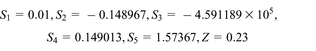
In this study, we are mainly concerned with the changes generated in the system by Ω under different conditions. The Si–Si system and related parameters S₁–S₅ and Z are definite values ⁵ as shown below

$$S_1=0.01,S_2=-0.148967,S_3=-4.591189\times {10}^5,S_4=0.149013,S_5=1.57367,Z=0.23$$

Phase portrait

The phase portrait ¹² is a geometric representation of the trajectories of a dynamical system in the phase plane and the axes are system state variables including X₁ and X₂ calculated from equations (1)–(4). From Figure 1(a), (c), and (e), the system is rather disordered and irregular for Ω = 0.46, 2.15, and 4, so that a preliminary determination of the dynamic behavior can be regarded as a non-periodic phenomenon for Ω = 0.46, 2.15, and 4. Furthermore, for Ω = 1.03, 3, and 4.7, the locus of the probe is in an ordered and regular state, as shown in Figure 1(b), (d), and (f), so that the system has periodic dynamic behavior.

Figure 1.

Phase portraits of probe tips at different Ω: (a) Ω = 0.46, (b) Ω = 1.03, (c) Ω = 2.15, (d) Ω = 3, (e) Ω = 4, and (f) Ω = 4.7.

Spectra analysis

After the displacement and velocity of probe tips obtained from equations (1)–(4), the responses of spectral analysis are then calculated by Fourier transformation using the results of X₁ and X₂. Figure 2 shows a spectral analysis for probe displacement and velocity response. Ω = 1.03 and Ω = 4 indicate periodic and non-periodic changes. In Figure 2(a) and (b), for a power spectrum with Ω = 1.03, the frequency responses of velocity and displacement both show periodic motion; for Ω = 4, the frequency becomes dense and irregular, as shown in Figure 2(c) and (d); in this case, the system is in irregular, non-periodic motion.

Figure 2.

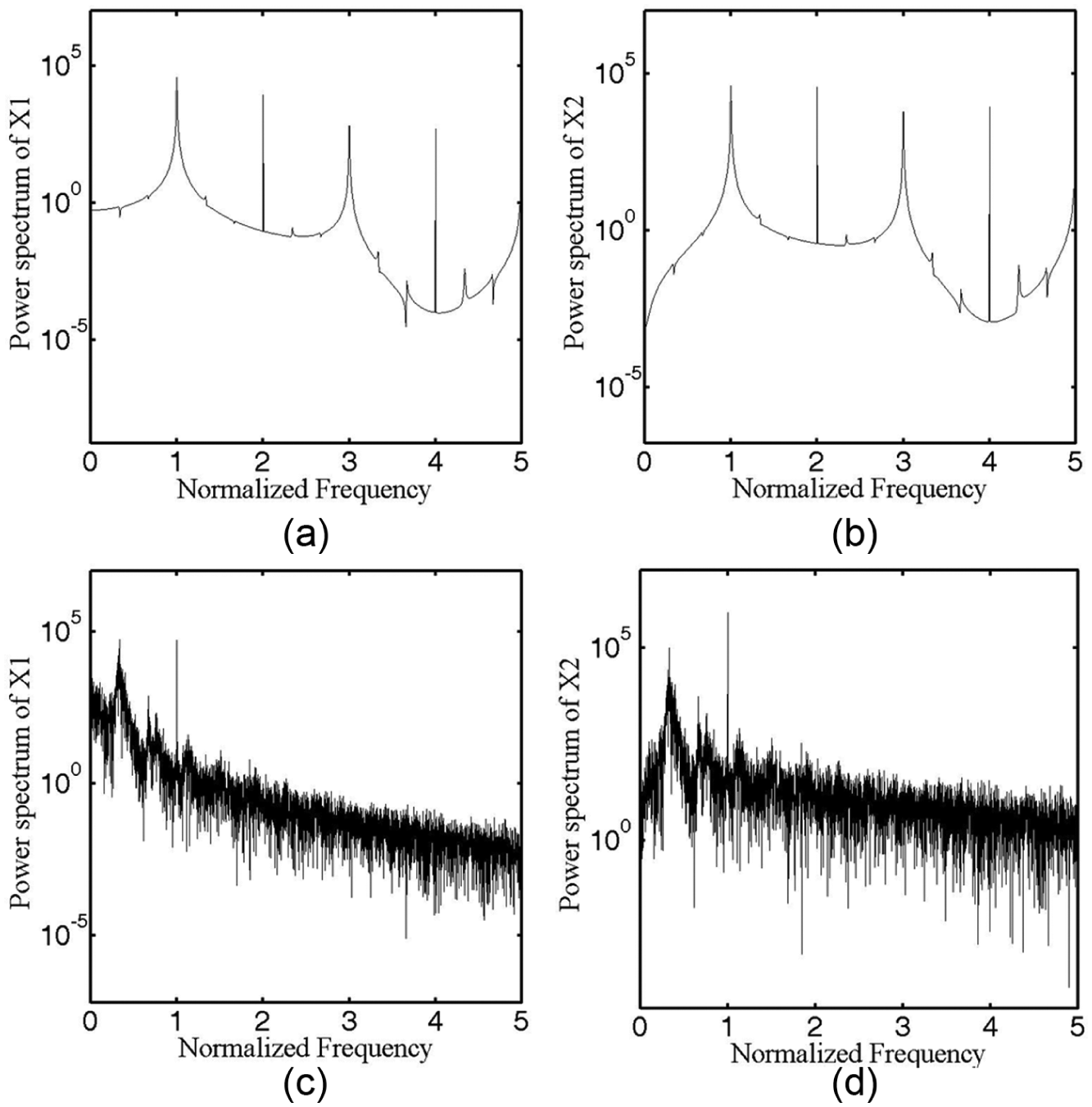
Responses of spectral analysis for displacement and velocity of probe tips: (a) and (b) are for Ω = 1.03 and (c) and (d) are for Ω = 4.

Bifurcation and Poincaré map analysis

In general, bifurcation diagrams ¹³ show the values visited or approached asymptotically (fixed points, periodic orbits, or chaotic attractors) of a system as a function of a bifurcation parameter (Ω) in AFM system. Poincaré map ¹⁴ is the intersection of a periodic orbit in the state space of a continuous dynamical system with a certain lower-dimensional subspace transversal to the flow of the system. In this study, Figure 3(a) and (b) plots the bifurcation diagrams of the tip displacement and the tip velocity, respectively, taking the Ω of the system as the bifurcation parameter. Figure 4(a)–(e) presents the local bifurcation diagrams of the microcantilever tip for the specific ranges of Ω. Figure 5(a)–(f) presents the Poincaré maps of the microcantilever tip trajectory at Ω = 0.46, 1.03, 2.15, 3, 4, and 4.7, respectively.

Figure 3.

(a) Bifurcation diagram for displacement of the probe tip and (b) bifurcation diagram for velocity of the probe tip.

Figure 4.

Local bifurcation diagrams for tip displacement using excitation frequency ratio as the bifurcation parameter: (a) 0.1 ≤ Ω < 0.84, (b) 1.75 ≤ Ω < 1.99, (c) 1.99 ≤ Ω < 2.45, (d) 3.45 ≤ Ω <4.12, and (e) 4.12 ≤ Ω < 4.57.

Figure 5.

Poincaré maps of probe tips with respect to changes of different excitation frequency ratio: (a) Ω = 0.46, (b) Ω = 1.03, (c) Ω = 2.15, (d) Ω = 3, (e) Ω = 4, and (f) Ω = 4.7.

Figure 4(a) shows that at lower values of Ω, that is, Ω < 0.84, both the displacement (X₁) and velocity (X₂) of the tip exhibit a chaos-nT response meaning the occurrence of chaotic and sub-harmonic motions alternately. Figure 5(a) presents the Poincaré map corresponding to Ω = 0.46, and the map has attractors that confirm the existence of chaotic behavior shown in the bifurcation diagrams. As the value of the excitation frequency ratio is increased from Ω = 0.84 to Ω = 1.75, AFM system performs T-periodic and sub-harmonic motions including 2T, 4T, and 5T. Figure 5(b) presents the Poincaré map at Ω = 1.03, and it exists at a single point to verify T-periodic motion. At Ω = 1.75, the stable motion is replaced by chaotic, as shown in Figure 4(b), and it also shows that the type of chaos-T motion is maintained over the excitation frequency ratio range of 1.75 ≤ Ω < 1.99. Thereafter, system behavior is replaced and repeated by the chaos-nT response over the interval of 1.99 ≤ Ω < 2.45 as shown in Figure 4(c). Figure 5(c) shows the Poincaré map at Ω = 2.15, and it occurs in chaotic motion. But for excitation frequency ratio in the range 2.45 ≤ Ω < 3.45, the tip performs T- and sub-harmonic motions and from Figure 5(d) the tip behaves 3T-periodic motion at Ω = 3. When Ω is increased over the interval 3.45 ≤ Ω < 4.12 and 4.12 ≤ Ω < 4.57, the tip exhibits chaos-T and chaos-nT motions as shown in Figure 4(d) and (f). When Ω = 4, the tip performs chaotic motion as shown in Figure 5(e). However, at Ω = 4.57, the multi-periodic motion is replaced by chaotic-nT motion, and the tip response includes both T- and sub-harmonic motions over the interval 4.57 ≤ Ω ≤ 5.0. Figure 5(f) presents the Poincaré map at Ω = 4.7, and the presence of three discrete points is observed to confirm the occurrence of 3T-periodic motion.

From the discussions above, it is clear that the dynamic response of the probe tip depends on the magnitude of the excitation frequency ratio. The various motions performed by the tip as the excitation frequency ratio increases from 0.1 to 5.0 are summarized in Table 1. In general, from the bifurcation diagrams, it can be seen that the displacement and velocity changes in the system result from synchronous vibration with the same changes of motion characteristics for periodic, sub-harmonic, and chaotic behaviors. The tip behavior for each interval is shown in Table 1. For 0.84 ≤ Ω < 1.75, 2.45 ≤ Ω < 3.45, and 4.57 ≤ Ω ≤ 5.0, the system presents either stable periodic or sub-harmonic motion. These three intervals belong to a more stable range, while chaotic behavior and periodic or sub-harmonic motion appears alternately for other intervals.

Table 1.

Analysis of dynamic behavior at different intervals.

Ω	[0.1, 0.84)	[0.84, 1.75)	[1.75, 1.99)	[1.99, 2.45)
Behavior	Chaos-nT	T-2T-4T-5T	Chaos-T	Chaos-nT
Ω	[2.45, 3.45)	[3.45, 4.12)	[4.12, 4.57)	[4.57, 5.0]
Behavior	T-nT, n=1-multi	Chaos-T	Chaos-nT	Multi-T

Maximum Lyapunov exponent

Lyapunov exponent is a quantity that characterizes the rate of separation of infinitesimally close trajectories. Quantitatively, two trajectories in phase space with initial separation diverge at a rate. The rate of separation can be different for different orientations of initial separation vector. Thus, there is a spectrum of Lyapunov exponents—equal in number to the dimensionality of the phase space. It is common to refer to the largest one as the maximum Lyapunov exponent (MLE) ¹⁵ because it determines a notion of predictability for a dynamical system. A positive MLE is usually taken as an indication that the system is chaotic. When the MLE is greater than zero, the system state is chaotic. On the other hand, if the MLE is smaller or equal to zero, the system is in non-chaotic or periodic motion. In Figure 6(a), (c), and (e), the MLE is greater than zero, and the dynamic behavior is chaotic; while in Figure 6(b), (d), and (f), where the MLE approaches zero in all three cases, the system is in a non-chaotic state. The dynamic behavior for each of these intervals can be verified in conjunction with a Poincaré map and phase portrait.

Figure 6.

Changes in maximum Lyapunov exponent of the probe tip under different excitation frequencies: (a) Ω = 0.46, (b) Ω = 1.03, (c) Ω = 2.15, (d) Ω = 3, (e) Ω = 4, and (f) Ω = 4.7.

Chaos control

As an example of chaos for dynamic analysis, and as the parameter for subsequent chaos control we used an excitation frequency ratio Ω = 0.46. PSO was used to search for optimized PD control parameters K_P and K_D for the output response of the AFM system to achieve the required performance.

PSO was proposed by Kennedy and Eberhart ¹¹ in 1995 based on the observed behavior of birds and bees when searching for food. More specifically, individual birds (bees) generate both memory and experience when searching for food in the location closest to them. As the search process proceeds, the individual experience is transferred to the flock (swarm) as a whole such that the entire flock (swarm) gradually converges to the same location. In PSO, every particle represents a candidate solution to the problem of interest and, just as an individual bird (or bee), searches initially within its own local region of the solution space in accordance with a particular speed and direction. Following each iteration, the search speed and search direction of each particle are updated in accordance with both the local experience of the particle and the global experience of the swarm. The process proceeds iteratively in this way until the specified termination criterion is achieved (typically a certain number of iterations performed or an error value less than a certain predefined tolerance). This is referred to as the PSO-PD controller (see Figure 7).

Figure 7.

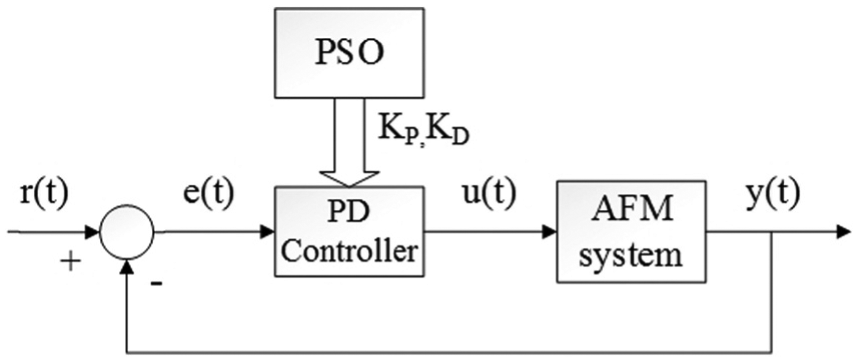
Block diagram showing how the optimal PD control parameters are found with PSO.

Mathematical model of the system with PD controller

In order to suppress chaos in the AFM system, input control item u(t) was added to equation (2) to obtain the following formula

$$\{\begin{array}{c}{\stackrel{.}{X}}_1=X_2\\ \begin{array}{l}{\stackrel{.}{X}}_2=-S_1{X}_2-X_1+S_2+\frac{S_3}{{(1-X_1-Z\sin (\Omega \tau ))}^8}+\frac{S_4}{{(1-X_1-Z\sin (\Omega \tau ))}^2}\\ +Z{\Omega }^2{S}_5\sin (\Omega \tau )+u(t)\end{array}\end{array}$$

(5)

To get the error signal $[e_1,e_2]$ to approach zero, the system output y(t) is subtracted from the system input r(t), as shown in equation (6). An error signal is obtained which provides the control item u(t) through the PD controller, as shown in equation (10), and the expression satisfies the condition shown below

$$\underset{t\to \infty }{lim}\left||r_i(t)-y_i(t)|\right|=\underset{t\to \infty }{lim}\left||e_i(t)|\right|\to 0,i=1,2$$

(6)

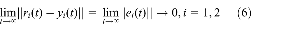
The error signal $E(t)=(r_1(t)-y_1(t),r_2(t)-y_2(t))=(e_1,e_2)$ is obtained which is substituted into equation (5), from which the following equations can be derived

$${\stackrel{·}{e}}_1=e_2$$

(7)

$$\begin{array}{c}\multicolumn{1}{c}{{\stackrel{·}{e}}_2=-S_1{e}_2-e_1+S_2+\frac{S_3}{{(1-X_1-Z\sin (\Omega \tau ))}^8}}\\ \multicolumn{1}{c}{+\frac{S_4}{{(1-X_1-Z\sin (\Omega \tau ))}^2}+Z{\Omega }^2{S}_5\sin (\Omega \tau )+u(t)}\end{array}$$

(8)

where

$$u(t)=K_P{e}_1+K_D{e}_2$$

(9)

where K_P and K_D are the proportional and differential gains of the two controllers, respectively.

Evaluation of system response characteristics

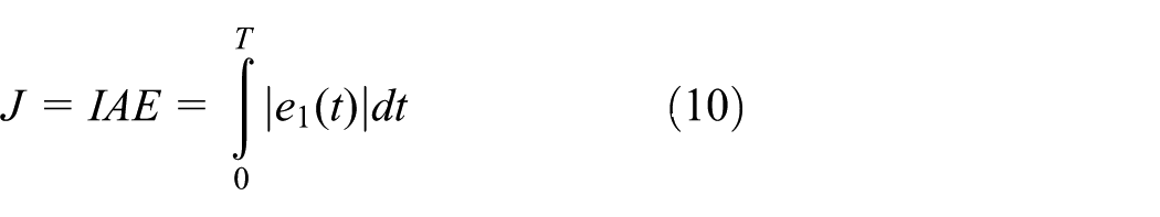
The entire system acts as a means for adjusting the search parameters of the PD controller. Accordingly, an adaptive function has to be used as a criterion for parameter quality. After the proportion of PD controller (differential parameter) has been determined, the adaptive function of equation (10) is used as a criterion for quality evaluation, and PSO is the search tool. The adaptive function used is the integral absolute error (IAE) of error signal e₁ which is used as a criterion for evaluation. The equation is shown below

$$J=\mathrm{IAE}=\underset{0}{\overset{T}{\int }}|e_1(t)|\mathrm{dt}$$

(10)

The design of PSO

To start with, the initial conditions for PSO are set; these include the learning constants, total number of particles in the swarm (n), the number of iterations, range of parameter search, and so on. Because a PD controller is used, there are two variables K_P and K_D, which provide initial position and velocity for 2 × n particles, the K_P and K_D parameters and plant AFM system operate in series, followed by the recording of an individual optimal solution and a global optimal solution for each of the particles. In the next step, the positions and velocities of the particles are updated and the inertial weight algorithm is used to update them. After a calculation to determine whether the adaptive function value IAE record represented by each of the particles is convergent or not (until the predetermined iteration ends), a set of optimal PD parameters is available. The operation flowchart is shown in Figure 8.

Figure 8.

Flowchart for PSO algorithm design.

Simulation and experimental result

If the chaotic behavior at Ω = 0.46 is used for control, the trajectory map for chaos is as shown in Figure 1(a). After the AFM system is combined with PD controller, this is added to the locus of the system at an arbitrary time, such that the locus can converge to near 0. In other words, the purpose is to converge the chaos locus so that is becomes stable. The result of locus control is shown in Figure 9.

Figure 9.

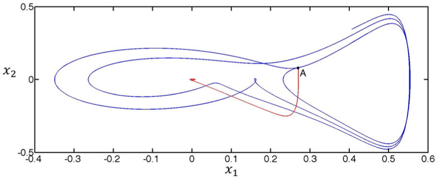
Trajectory map of plant AFM system.

To observe the effect of control, followed by analysis using an error signal with the same excitation frequency ratio, the AFM system simulates error signals e₁ and e₂ for 100 s, and control can be added at any selected time. We chose 60th second to add control and found that the unstable signal became stable within about 65 s. The control effect is as shown in Figure 10.

Figure 10.

Error signal responses e₁ and e₂ with added control.

In this study, the circuit power was restricted to ±12 V as an upper limit so that the control item u(t) was kept within −10, as shown in Figure 11(a). This was done as a reference for subsequent circuit implementation. Thus, the search range for K_P and K_D parameters is limited to 0–20. Furthermore, the initial values of the K_P and K_D parameters were set as 5, 10, and 15 to prove the robustness of PSO search, as shown in Figure 11(c) and (d). It was discovered that when the iteration was between 50 and 60, the PSO search converges to be optimal and there is consistent correspondence with the performance indicator IAE in Figure 11(b).

Figure 11.

(a) Time response diagram of control item u(t), (b) parameter performance indicator IAE, (c) iteration graph for search parameter K_P, and (d) iteration graph for search parameter K_D.

Conclusion

The main purpose of this study was to investigate the dynamic characteristics of the AFM system with variation in the excitation frequency ratio and to develop a PD controller using PSO to suppress the chaotic motion. Changes in Ω have a marked effect on the AFM system. Phase portrait, spectral analysis, bifurcation diagram, Poincaré map, and the MLE were used to observe and verify the generation of chaotic behavior. The results obtained by each analytical method are consistent and shown in Table 1. Stable operation of the AFM is interrupted from time to time by chaotic behavior. This is generated intermittently in periodic or sub-harmonic period form during three intervals of 0.84 ≤ Ω < 1.75, 2.45 ≤ Ω < 3.45, and 4.57 ≤ Ω ≤ 5.0, so that an increase in excitation frequency ratio influences the system absolutely. In our study, optimization parameters were found through a PD controller by the use of PSO to guarantee for restraining chaos over five intervals of 0.1 ≤ Ω < 0.84, 1.75 ≤ Ω < 1.99, 1.99 ≤ Ω ≤ 2.45, 3.45 ≤ Ω < 4.12, and 4.12 ≤ Ω < 4.57. The quality of parameters K_P and K_D was determined with reference to the indicator IAE. The results may be useful as reference criteria for subsequent implementation in AFM system circuitry to reduce or avoid the incidence of this kind of instability and non-periodic motion in the measurement precision of AFM systems.